Exact solitary wave solutions for a discrete $\lambda\phi^{4}$ field theory in $1+1$ dimensions

Abstract

We have found exact, periodic, time-dependent solitary wave solutions of a discrete $\phi^{4}$ field theory model. For finite lattices, depending on whether one is considering a repulsive or attractive case, the solutions are either Jacobi elliptic functions ${\rm sn}(x,m)$ (which reduce to the kink function $\tanh(x)$ for $m\rightarrow 1$), or they are ${\rm dn}(x,m)$ and ${\rm cn}(x,m)$ (which reduce to the pulse function ${\rm sech}(x)$ for $m\rightarrow 1$). We have studied the stability of these solutions numerically, and we find that our solutions are linearly stable in most cases. We show that this model is a Hamiltonian system, and that the effective Peierls-Nabarro barrier due to discreteness is zero not only for the two localized modes but even for all three periodic solutions. We also present results of numerical simulations of scattering of kink–anti-kink and pulse–anti-pulse solitary wave solutions.

I Introduction

Discrete nonlinear equations are ubiquitous and play an important role in diverse physical contexts clark ; scott . Some examples of integrable discrete equations include Ablowitz-Ladik (AL) lattice AL and Toda lattice toda . Certain non-Abelian discrete integrable models are also known nonabel . There are many non-integrable discrete nonlinear equations such as discrete sine-Gordon (DSG) DSG1 ; DSG2 , discrete nonlinear Schrödinger (DNLS) equation DNLS and the Fermi-Pasta-Ulam (FPU) problem ford . DSG is a physical realization of the dynamics of dislocations in crystals where it is known as the Frenkel-Kontorova model nabarro . It also arises in the context of ferromagnets with planar anisotropy mikeska , adsorption on a crystal lattice and pinned charge-density waves sacco . Similarly, DNLS plays a role in the propagation of electromagnetic waves in doped glass fibers fibers and other optical waveguides OP , and it describes Bose-Einstein condensates in optical lattices ST . FPU has served as a fertile paradigm for understanding solitons, discrete breathers, intrinsic localized modes, chaos, anomalous transport in low-dimensional systems and the fundamentals of statistical mechanics ford . A discrete double well or discrete $\phi^{4}$ equation is a model for structural phase transitions dphi4 , and may be relevant for a better understanding of the collisions of relativistic kinks luis .

Obtaining exact (soliton-like) solutions is always desirable, particularly for discrete systems where the notion of a discreteness (or Peierls-Nabarro) barrier PN ; peyrard is an important one in that its absence is a likely indication of integrability, e.g. in the AL case scott . In addition, exact solutions allow one to calculate certain important physical quantities analytically as well as they serve as diagnostics for simulations. Recently derived summation identities khare involving Jacobi elliptic functions stegun ; byrd led to exact periodic solutions of a modified DNLS equation dnls . In this paper we exploit similar identities to obtain exact periodic solutions of the discrete $\phi^{4}$ model.

The paper is organized as follows. In the next section we summarize the exact solitary wave solutions of the continuum $\phi^{4}$ model. In Sec. III, by identifying the relevant elliptic function identities, we derive a discrete $\phi^{4}$ model which allows for exact solutions. We then obtain these solutions and study their stability. In Sec. IV we explicitly write down the corresponding Hamiltonian dynamics using a modified Poisson bracket algebra. Sec. V contains numerical results for the scattering of both kink- and pulse-like solitary waves. Kink–anti-kink collisions appear to create a breather with some radiation, and pulse–anti-pulse collisions lead to a flip and little radiation. In Sec. VI we compute the energy of the solitary waves, and show that the Peierls-Nabarro barrier PN ; peyrard due to discreteness is zero not only for the two localized solutions but even for the three periodic solutions. Finally, we summarize our main findings in Sec. VII.

II Continuum solitary waves

The double-well potential with the coupling parameter $\lambda$ and the two minima at $\phi=\pm a$

$$V=\frac{\lambda}{4}\ (\phi^{2}-a^{2})^{2}$$ (1)

leads to the following relativistic field equation

$$-\frac{\partial^{2}\phi}{\partial t^{2}}+\frac{\partial^{2}\phi}{\partial x^{2}}-\lambda\phi(\phi^{2}-a^{2})=0\>.$$ (2)

For $\lambda>0$, if one assumes a moving periodic solution with velocity $v$ in terms of the Jacobi elliptic function ${\rm sn(x,m)}$ with modulus $m$

$$\phi(x,t)=Aa~{}{\rm sn}\left[\beta(x+x_{0}-vt),m\right]$$ (3)

one finds that

$$-\frac{\partial^{2}\phi(x,t)}{\partial t^{2}} +\frac{\partial^{2}\phi(x,t)}{\partial x^{2}}$$ (4)

$$=-\beta^{2}a~{}(1-v^{2})~{}[(1+m)~{}{\rm sn}-2m~{}{\rm sn}^{3}]\>,$$

where we have suppressed the argument of ${\rm sn}$. Matching terms proportional to ${\rm sn}$ and ${\rm sn}^{3}$ we find we have a moving periodic solution with

$$\beta =\left[\frac{\lambda a^{2}}{(1-v^{2})(1+m)}\right]^{1/2},$$

$$A =\sqrt{\frac{2m}{1+m}}.$$ (5)

The usual kink solitary wave is obtained in the limit $m~{}\rightarrow~{}1$. Since

$${\rm sn}(x,1)=\tanh(x)\>,$$ (6)

we obtain

$$\phi(x,t)=a\tanh\Biggl{\{}\left[\frac{\lambda a^{2}}{2(1-v^{2})}\right]^{1/2}(x+x_{0}-vt)\Biggr{\}}\>.$$ (7)

If instead $\lambda<0$, then there are $\mathrm{dn}$ Jacobi elliptic function solutions to the field equations. Assuming

$$\phi(x,t)=Aa~{}{{\rm dn}}\left[\beta(x+x_{0}-vt),m\right]\>,$$ (8)

and matching terms proportional to ${\rm dn}$ and ${\rm dn}^{3}$, we find a moving periodic pulse solution with

$$\beta =\left[\frac{-\lambda a^{2}}{(1-v^{2})(2-m)}\right]^{1/2},$$

$$A =\sqrt{\frac{2}{2-m}}\>.$$ (9)

In fact, there is another pulse solution in terms of the Jacobi elliptic function of ${\rm cn}$ type. Assuming

$$\phi(x,t)=Aa~{}{{\rm cn}}\left[\beta(x+x_{0}-vt),m\right]\>.$$ (10)

Matching terms proportional to ${\rm cn}$ and ${\rm cn}^{3}$ we find we have a moving periodic solution with

$$\beta =\left[\frac{-\lambda a^{2}}{(1-v^{2})(2m-1)}\right]^{1/2},$$

$$A =\sqrt{\frac{2m}{2m-1}}.$$ (11)

Note that this solution is valid only if $m>1/2$.

The usual pulse solitary wave is obtained in the limit $m\rightarrow 1$. Since

$${\rm dn}(x,1)={\rm cn}(x,1)={\rm sech}(x)\>,$$ (12)

we obtain

$$\phi(x,t)=a\sqrt{2}{\rm sech}\left[\left(\frac{-\lambda a^{2}}{1-v^{2}}\right)^{1/2}(x+x_{0}-vt)\right]\>.$$ (13)

Note that similar solutions and their stability were considered by Aubry in the context of structural phase transitions aubry . In the rest of this paper we will refer to the $\mathrm{sn}$ solutions as kink-like, and to the $\mathrm{dn}$ and $\mathrm{cn}$ solutions as pulse-like.

III Discretization of $\lambda\phi^{4}$ field theory

A naive discretization of the field equation above is

$$-\ddot{\phi}_{n}+\frac{1}{\epsilon^{2}}(\phi_{n+1}+\phi_{n-1}-2\phi_{n})+\lambda\phi_{n}(a^{2}-\phi_{n}^{2})=0\>,$$ (14)

where $\epsilon$ is the lattice parameter and the overdots represent time derivatives. However, this equation does not admit solutions of the form

$$\phi_{n}(t)=Aa~{}{{\rm sn}}(\beta[(n+c)\epsilon-vt],m),$$ (15)

where $c$ is an arbitrary constant. To find solutions, one has to modify the naive discretization. The key for understanding how to modify the equation comes from the following identities khare of the Jacobi elliptic functions

${\rm sn}$:

$$m~{}{\rm sn}(x,m)^{2} \left[{\rm sn}(x+\beta,m)+{\rm sn}(x-\beta,m)\right]$$ (16)

$$=\ {\rm ns}^{2}(\beta,m)\bigl{[}{\rm sn}(x+\beta,m)+{\rm sn}(x-\beta,m)\bigr{]}$$

$$-2{\rm cs}(\beta,m){\rm ds}(\beta,m){\rm sn}(x,m)\>,$$

${\rm cn}$:

$$m~{}{\rm cn}(x,m)^{2} \left[{\rm cn}(x+\beta,m)+{\rm cn}(x-\beta,m)\right]$$ (17)

$$=\ -{\rm ds}^{2}(\beta,m)\bigl{[}{\rm cn}(x+\beta,m)+{\rm cn}(x-\beta,m)\bigr{]}$$

$$+2{\rm cs}(\beta,m){\rm ns}(\beta,m){\rm cn}(x,m)\>,$$

and ${\rm dn}$:

$${\rm dn}(x,m)^{2} \left[{\rm dn}(x+\beta,m)+{\rm dn}(x-\beta,m)\right]$$ (18)

$$=\ -{\rm cs}^{2}(\beta,m)\bigl{[}{\rm dn}(x+\beta,m)+{\rm dn}(x-\beta,m)\bigr{]}$$

$$+2{\rm ds}(\beta,m){\rm ns}(\beta,m){\rm dn}(x,m)\>,$$

where

$$ns=\frac{1}{{\rm sn}(x,m)}\>,\quad cs=\frac{{\rm cn}(x,m)}{{\rm sn}(x,m)}\>,\quad ds=\frac{{\rm dn}(x,m)}{{\rm sn}(x,m)}\>.$$ (19)

It will be useful later to rewrite these identities in the form:

$${\rm sn}(x+\beta,m) +{\rm sn}(x-\beta,m)$$ (20)

$$= \ 2\ {\rm cs}(\beta,m)\ {\rm ds}(\beta,m)\ {\rm sn}(x,m)$$

$$\times[{\rm ns}^{2}(\beta,m)-m\ {\rm sn}(x,m)^{2}]^{-1},$$

$${\rm cn}(x+\beta,m) +{\rm cn}(x-\beta,m)$$ (21)

$$= \ 2\ {\rm cs}(\beta,m)\ {\rm ns}(\beta,m)\ {\rm cn}(x,m)$$

$$\times[{\rm ds}^{2}(\beta,m)+m\ {\rm cn}(x,m)^{2}]^{-1},$$

and

$${\rm dn}(x+\beta,m) +{\rm dn}(x-\beta,m)$$ (22)

$$= \ 2\ {\rm ds}(\beta,m)\ {\rm ns}(\beta,m)\ {\rm dn}(x,m)$$

$$\times[{\rm dn}(x,m)^{2}+{\rm cs}^{2}(\beta,m)]^{-1}.$$

For the sake of brevity, in what follows we will suppress the modulus $m$ in the argument of the Jacobi elliptic functions, except when needed for added clarity.

III.1 Static lattice solutions

Consider the naive lattice equation:

$$\frac{1}{\epsilon^{2}}\bigl{(}\phi_{n+1}+\phi_{n-1}-2\phi_{n}\bigr{)}+\lambda\phi_{n}(a^{2}-\phi_{n}^{2})=0\>.$$ (23)

Here $\phi_{n}\equiv\phi[\beta\epsilon(n+c),m]$. A general ansatz to modify the solution is to multiply the second difference operator by the factor $(1-\alpha\phi_{n}^{2})$, with $\alpha$ chosen so that we get a consistent set of equations. That is, we consider instead the equation:

$$\frac{1-\alpha\phi_{n}^{2}}{\epsilon^{2}}\bigl{(}\phi_{n+1}+\phi_{n-1}-2\phi_{n}\bigr{)}+\lambda\phi_{n}(a^{2}-\phi_{n}^{2})=0.$$ (24)

Using $\alpha$ to eliminate the $\phi_{n}^{3}$ term leads to the result

$$\alpha=\lambda\epsilon^{2}/2.$$ (25)

This implies, in the static case, that the lattice equation is just a smeared discretization of the $\phi_{n}^{3}$ term. Namely, one merely needs to study the lattice equation:

$$\frac{1}{\epsilon^{2}}\bigl{(}\phi_{n+1}+\phi_{n-1}-2\phi_{n}\bigr{)}=\frac{\lambda\phi_{n}^{2}}{2}\bigl{(}\phi_{n+1}+\phi_{n-1}\bigr{)}-\lambda\phi_{n}a^{2}.$$ (26)

Assume a solution of the form (for $\lambda>0$)

$$\phi_{n}=Aa~{}{\rm sn}_{n}\,,$$ (27)

where ${\rm sn}_{n}$ denotes ${\rm sn}[\beta\epsilon(n+c),m]$ with $c$ being an arbitrary constant. Note that we only need to consider $c$ between 0 and 1/2 (half the lattice spacing). On matching the coefficients of ${\rm sn}_{n}$ and ${\rm sn}_{n+1}+{\rm sn}_{n-1}$ we obtain

$$A^{2}a^{2}=\frac{(1+m)~{}{\rm sn}^{2}(\beta\epsilon)}{\lambda\epsilon^{2}},$$ (28)

and

$$\lambda a^{2}=\frac{2}{\epsilon^{2}}\left[1-{\rm dn}(\beta\epsilon){\rm cn}(\beta\epsilon)\right]\>.$$ (29)

In the continuum limit ($\epsilon\rightarrow 0$), we get

$$\beta^{2}=\frac{\lambda a^{2}}{1+m};~{}~{}~{}A^{2}=\frac{2m}{1+m}\>,$$ (30)

which agrees with our continuum result (2.5) with $v=0$. Also as $m\rightarrow 1$ we recover the usual kink solution

$$\phi_{n}=a\ \tanh[\beta\epsilon(n+c)]\,.$$ (31)

If instead, we have $\lambda<0$ and we assume

$$\phi_{n}=Aa~{}{\rm dn}_{n},$$ (32)

we obtain:

$$A^{2}a^{2}=-\frac{2m}{\lambda\epsilon^{2}}\frac{{\rm sn}^{2}(\beta\epsilon)}{{\rm cn}^{2}(\beta\epsilon)}\>,$$ (33)

and

$$\lambda a^{2}\frac{2}{\epsilon^{2}}\left[1-\frac{{\rm dn}(\beta\epsilon)}{{\rm cn}^{2}(\beta\epsilon)}\right]\>.$$ (34)

In the limit when the lattice spacing $\epsilon$ goes to zero, we obtain

$$\beta^{2}=-\frac{\lambda a^{2}}{2-m};~{}~{}~{}A^{2}=\frac{2}{2-m},$$ (35)

same as the continuum case (2.9) with $v=0$.

For $\lambda<0$ we also have a possible solution of the form

$$\phi_{n}=Aa~{}{\rm cn}_{n},$$ (36)

we obtain:

$$A^{2}a^{2}=-\frac{2m}{\lambda\epsilon^{2}}\frac{{\rm sn}^{2}(\beta\epsilon)}{{\rm dn}^{2}(\beta\epsilon)},$$ (37)

and

$$\lambda a^{2}=\frac{2}{\epsilon^{2}}\left[1-\frac{{\rm cn}(\beta\epsilon)}{{\rm dn}^{2}(\beta\epsilon)}\right].$$ (38)

Again taking the lattice spacing to zero, we obtain

$$\beta^{2}=-\frac{\lambda a^{2}}{2m-1};~{}~{}~{}A^{2}=\frac{2m}{2m-1},$$ (39)

same as the continuum case (2.11) with $v=0$. Note that as before this solution is only valid if $m>1/2$. For both these solutions, as $m\rightarrow 1$, we get our previous continuum solution:

$$\phi_{n}=\sqrt{2}a\ {\rm sech}[\beta\epsilon(n+c)]\>.$$ (40)

III.2 Stability of solutions

Figure 1: (Color online) Kink-like ($\lambda>0$) case: N-dependence of the lowest eigenvalue, $\omega_{1}^{2}$, for $\lambda=1,\ a=1$, and various values of the elliptic modulus $m$.

Figure 2: (Color online) Kink-like ($\lambda>0$) case: N-dependence of the lattice spacing, $\epsilon$, for $\lambda=1,\ a=1$, and various values of $m$.

Figure 3: (Color online) Pulse-like ($\lambda<0$) ${\rm dn}$ case: N-dependence of the lowest eigenvalue, $\omega_{1}^{2}$, for $\lambda=-1,\ a=1.5$, and various values of $m$.

Figure 4: (Color online) Pulse-like ($\lambda<0$) ${\rm dn}$ case: N-dependence of the lattice spacing, $\epsilon$, for $\lambda=-1,\ a=1.5$, and various values of $m$.

Let us now discuss the stability of these static solutions. To that purpose, let us expand

$$\phi_{n}=\phi_{n}^{(s)}+\psi_{n}\exp(-i\omega t),$$

where $\phi_{n}^{(s)}$ is the known solitary wave exact solution and $\psi_{n}$ is a small perturbation. Then we find that to the lowest order in $\psi_{n}$ the stability equation is

$$\omega^{2}\psi_{n}+\frac{1}{\epsilon^{2}}(\psi_{n+1}+\psi_{n-1}-2\psi_{n})$$

$$-\lambda\ \psi_{n}\phi_{n}^{(s)}[\phi^{(s)}_{n+1}+\phi^{(s)}_{n-1}]$$

$$+\lambda\psi_{n}a^{2}-\frac{\lambda\phi_{n}^{2}}{2}(\psi_{n+1}+\psi_{n-1})=0\>.$$ (41)

Using the identities (20), (3.8) and (22), the combination $[\phi^{(s)}_{n+1}+\phi^{(s)}_{n-1}]$ can be written as a function of $\phi_{n}$ alone. Thus schematically we have

$$\bigl{(}\omega^{2}-f_{n}\bigr{)}\psi_{n}\ +\ g_{n}\bigl{(}\psi_{n+1}+\psi_{n-1}\bigr{)}\ =\ 0\>,$$ (42)

or

$$\psi_{n+1}+\psi_{n-1}+h_{n}\psi_{n}=0\>,$$ (43)

with

$$h_{n}=\frac{\omega^{2}-f_{n}}{g_{n}}\>,$$ (44)

where $f_{n}$ and $g_{n}$ are well defined functions. We also have that the solutions are periodic on the lattice with $N$ sites ($\psi_{n+N}=\psi_{n}$). If we write the system of $N$ equations in matrix form, as

$$\mathbf{A}\ [\psi]\ =\ \omega^{2}\ [\psi],$$ (45)

then the condition for nontrivial solutions is that

$$\mathrm{Det}\ |\mathbf{A}-\omega^{2}\mathbf{1}|=0.$$ (46)

In our simulations we require that the solution has exactly one period in the model space. Therefore, the equations for $\beta$ and $A$ are supplemented by the equations

$$N\beta\epsilon\ =\ 4\ K(m)\>,$$ (47)

for solutions, $\phi_{n}=\mathrm{sn}(\beta n\epsilon)$ or $\phi_{n}=\mathrm{cn}(\beta n\epsilon)$, and

$$N\beta\epsilon\ =\ 2\ K(m)\>,$$ (48)

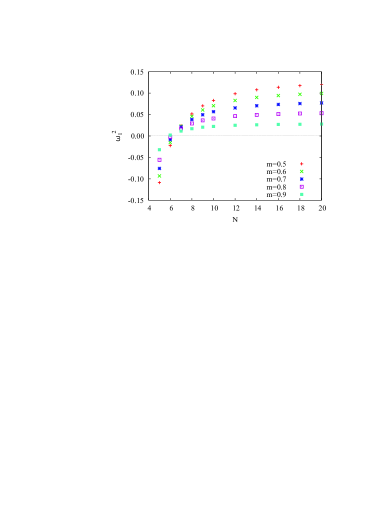
when $\phi_{n}=\mathrm{dn}(\beta n\epsilon)$. Here $K(m)$ is the complete elliptic integral of the first kind stegun ; byrd . Hence, once the parameters $m$, $\lambda$ and $a$ are specified, we need to solve a system of equations for $\beta$, $\epsilon$, and $A$, i.e. we have to solve Eqs. (28, 29, 47) or Eqs. (33, 34, 48), or Eqs. (37, 38, 47), for the solutions $\mathrm{sn}$, $\mathrm{dn}$, and $\mathrm{cn}$, respectively, for $\beta$, $\epsilon$, and $A$ as a function of N.

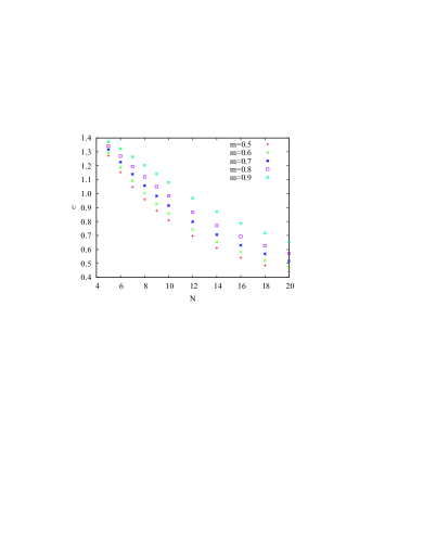
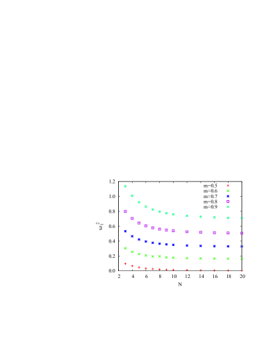
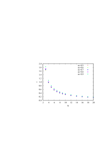
Typical results are depicted in Figs. 1 and 2 for kink-like ${\rm sn}$ solutions, and in Figs. 3 and 4, for pulse-like ${\rm dn}$ solutions, respectively. Similar results can also be obtained in the case of the ${\rm cn}$-type pulse solution. For the case of the kink-like solutions and our choice of parameters, we find from Fig. 1, that stability requires $N>7$ lattice sites. In the pulse-like case, we find stability for arbitrary values of $N$. The magnitude of the lowest eigenvalues increases with $N$ in the kink-like case, while it decreases with N for pulse-like solutions. For fixed $m$, $\lambda$, and $A$, the lattice spacing, $\epsilon$, is not an independent quantity, but it is a well-defined function of $N$. As seen from Figs. 2 and 4, the lattice spacing, $\epsilon$, is always a decreasing function of $N$.

IV Hamiltonian dynamics

In this section we demonstrate that our discrete model is a Hamiltonian system. The equation which the static solutions obey, Eq. (24), can be written as:

$$\frac{1}{\epsilon^{2}}\bigl{(}\phi_{n+1}+\phi_{n-1}-2\phi_{n}\bigr{)}+\lambda\frac{\phi_{n}(a^{2}-\phi_{n}^{2})}{1-\alpha\phi_{n}^{2}}=0.$$ (49)

We recognize that this equation can be derived from the potential function

$$V_{0}[\phi_{n}]=\sum_{n}\frac{(\phi_{n+1}-\phi_{n})^{2}}{2\epsilon^{2}}+\lambda\sum_{n}\int d\phi_{n}\frac{\phi_{n}(a^{2}-\phi_{n}^{2})}{1-\alpha\phi_{n}^{2}}.$$ (50)

Performing the integral we obtain explicitly:

$$V_{0}[\phi_{n}]= \sum_{n}\frac{(\phi_{n+1}-\phi_{n})^{2}}{2\epsilon^{2}}$$ (51)

$$\ -\ \lambda\frac{\phi_{n}^{2}}{2\alpha}\ +\ \lambda(a^{2}\alpha-1)\ \frac{\ln(1-\alpha\phi_{n}^{2})}{2\alpha^{2}}.$$

One easily verifies that

$$-(1-\alpha\phi_{n}^{2})\ \frac{\partial V_{0}}{\partial\phi_{n}}\ =\ \frac{1-\alpha\phi_{n}^{2}}{\epsilon^{2}}\bigl{(}\phi_{n+1}+\phi_{n-1}-2\phi_{n}\bigr{)}$$

$$\ +\ \lambda\phi_{n}(a^{2}-\phi_{n}^{2}).$$ (52)

The continuum limit $\alpha\rightarrow 0$ (or $\epsilon\rightarrow 0$) of the last two terms in Eq. (51) is given by

$$\frac{\lambda}{4}(\phi_{n}^{2}-a^{2})^{2}\ -\ \frac{\lambda}{4}a^{4}\>.$$ (53)

We will now show that if we want our class of solutions to be the static limit of a Hamiltonian dynamical system, that we will be able to have single solitary waves obey a simple equation, but general solutions will obey a more complicated dynamics with terms proportional to ${\dot{\phi}}^{2}$. For simplicity we will assume that the Hamiltonian takes the form:

$$H=\sum_{n}\left(\frac{\pi^{2}_{n}}{2}\,g[\phi_{n}]\ +\ V[\phi_{n}]\right),$$ (54)

with $V$ given by $V_{0}$ in Eq. (51) plus possibly some additional terms that vanish in the continuum limit. Here $\pi_{n}$ is the conjugate momentum and $g[\phi_{n}]$ a weight function. For generality we will assume, as in the case of the discrete nonlinear Schrödinger (DNLS) equation dnls ; das , that an extended Poisson bracket structure exists, namely:

$$\left\{\phi_{m},\pi_{n}\right\}=\delta_{nm}f[\phi_{n}],$$ (55)

and

$${\dot{\phi}}_{n}=\left\{\phi_{n},H\right\} =\frac{\partial H}{\partial\pi_{m}}\left\{\phi_{n},\pi_{m}\right\}=f[\phi_{n}]\frac{\partial H}{\partial\pi_{n}},$$

$${\dot{\pi}}_{n}=\left\{\pi_{n},H\right\} =\frac{\partial H}{\partial\phi_{m}}\left\{\pi_{n},\phi_{m}\right\}=-f[\phi_{n}]\frac{\partial H}{\partial\phi_{n}}.$$

From our ansatz, Eq. (54), we obtain the first order equations:

$${\dot{\phi}}_{n}=\pi_{n}f[\phi_{n}]g[\phi_{n}]\equiv\pi_{n}h[\phi_{n}],$$ (57)

and

$${\dot{\pi}}_{n}=-f[\phi_{n}]\left(\frac{\pi_{n}^{2}}{2}\frac{\partial g}{\partial\phi_{n}}+\frac{\partial V}{\partial\phi_{n}}\right).$$ (58)

This leads to the following second order differential equation for $\phi_{n}$

$${\ddot{\phi}}_{n}=-f[\phi_{n}]h[\phi_{n}]\frac{\partial V}{\partial\phi_{n}}+{\dot{\phi}}^{2}\left(\frac{1}{h}\frac{\partial h}{\partial\phi_{n}}-\frac{f}{2h}\frac{\partial g}{\partial\phi_{n}}\right).$$ (59)

For this equation to have the previously found static solitary waves, as well as the correct continuum limit, we need only that

$$f[\phi_{n}]h[\phi_{n}]=f^{2}[\phi_{n}]g[\phi_{n}]=1-\alpha\phi_{n}^{2}.$$ (60)

The two simplest cases are: (a) $f=1$ (ordinary Poisson brackets) and (b) $h=1$ (extended Poisson brackets). First consider the case $f=1$. This requires

$$h[\phi_{n}]=g[\phi_{n}]=1-\alpha\phi_{n}^{2}.$$ (61)

From this we get, if we choose $V=V_{0}$ with $V_{0}$ given by Eq. (51), the equation:

$$\ddot{\phi}_{n}\ =\ \frac{1-\alpha\phi_{n}^{2}}{\epsilon^{2}}\bigl{(}\phi_{n+1}+\phi_{n-1}-2\phi_{n}\bigr{)}$$ (62)

$$\ +\ \lambda\phi_{n}(a^{2}-\phi_{n}^{2})\ -\ \frac{\alpha{\dot{\phi}_{n}}^{2}\phi_{n}}{1-\alpha\phi_{n}^{2}}.$$

For $\alpha=\lambda{\epsilon^{2}}/{2}$ this equation has the previously found static lattice solitary wave solutions as well as the correct continuum limit. For the case $h=1$, this leads to

$$f=1-\alpha\phi_{n}^{2}\>,~{}~{}~{}g=(1-\alpha\phi_{n}^{2})^{-1}\>.$$ (63)

We find that for $V=V_{0}$ the equation of motion again becomes the same as Eq. (4.14).

Unfortunately the presence of the ${\dot{\phi}}^{2}$ term does not allow for single elliptic time dependent solitary wave solutions that are of the form ${\rm sn}[\beta(x-ct)]$, ${\rm cn}[\beta(x-ct)]$ or ${\rm dn}[\beta(x-ct)]$ where $x=n\epsilon$. This is because the second derivative of the ${\rm sn}$ and ${\rm dn}$ (or ${\rm cn}$) functions contains both linear as well as cubic terms, and the quantity ${\dot{\phi}}^{2}$ is a quartic polynomial in ${\rm sn}$ or ${\rm dn}$ (or ${\rm cn}$). Thus the last term is equivalent to a non-polynomial potential when applied to a single elliptic function solution. Therefore in order to obtain a simple elliptic function solution in the time dependent case, one must add a non-polynomial potential to $V_{0}$ which is chosen to exactly cancel the last term when evaluated for a single elliptic solitary wave solution of the form ${\rm sn}[\beta(x-ct)]$, ${\rm cn}[\beta(x-ct)]$ or ${\rm dn}[\beta(x-ct)]$. This means that to obtain an equation that is derivable from a Lagrangian or a Hamiltonian we should add to the static potential $V_{0}$ an additional contribution $\Delta V$ such that

$$(1-\alpha\phi_{n}^{2})\ \frac{\partial\Delta V}{\partial\phi_{n}}=-\frac{\alpha\phi_{n}{\dot{\phi}_{n}}^{2}}{1-\alpha\phi_{n}^{2}},$$ (64)

where $\phi_{n}$ is a single solitary wave described by a time translated elliptic function. It will turn out that $\Delta V$ needed to obtain a simple solution of the elliptic kind will depend on the velocity squared of the solitary wave as well as the type of solution (pulse- or kink-like).

In general we have that the Hamiltonian dynamics leads to

$${\ddot{\phi}}_{n}=-fh\frac{\partial V_{0}+\Delta V}{\partial\phi_{n}}+{\dot{\phi}_{n}}^{2}\left(\frac{1}{h}\frac{\partial h}{\partial\phi_{n}}-\frac{f}{2h}\frac{\partial g}{\partial\phi_{n}}\right).$$ (65)

Since $fh=1-\alpha\phi_{n}^{2}$ and $h=fg$, it follows that

$$\frac{1}{h}\frac{\partial h}{\partial\phi_{n}}-\frac{f}{2h}\frac{\partial g}{\partial\phi_{n}}=-\frac{\alpha\phi_{n}}{1-\alpha\phi_{n}^{2}},$$ (66)

from where the above condition for $\Delta V$ follows readily. For the single solitary wave solutions of the ${\rm sn}$, ${\rm cn}$ and ${\rm dn}$ type one wants to choose

$$\frac{\partial\Delta V}{\partial\phi_{n}}=\frac{a_{1}\phi_{n}^{5}+a_{2}\phi_{n}^{3}+a_{3}\phi_{n}}{(1-\alpha\phi_{n}^{2})^{2}},$$ (67)

with $a_{i}$ dependent on the choice of elliptic function, in order to cancel the effect of the ${\dot{\phi}}^{2}$ terms in the corresponding equation of motion.

Integrating, we get for $\Delta V$

$$\Delta V\ =\ \frac{a_{1}\phi^{2}}{2\alpha^{2}}+\frac{1}{2(1-\alpha\phi^{2})}\left(\frac{a_{1}}{\alpha^{3}}+\frac{a_{2}}{\alpha^{2}}+\frac{a_{3}}{\alpha}\right)$$

$$+\left(\frac{a_{1}}{\alpha^{3}}+\frac{a_{2}}{2\alpha^{2}}\right){\rm ln}(1-\alpha\phi^{2}).$$ (68)

If we assume a soliton solution of the form

$$\phi_{n}=Aa~{}{\rm sn}\Bigl{\{}\beta[(n+c)\epsilon-vt],m\Bigr{\}}\>,$$ (69)

where $c$ is an arbitrary constant, then

$${\dot{\phi}_{n}}^{2}=\beta^{2}v^{2}(Aa)^{2}[1-(1+m)\ {\rm sn}^{2}+m\ {\rm sn}^{4}],$$ (70)

which leads to

$$a_{1}\ =\ -\ m\alpha\left(\frac{\beta v}{Aa}\right)^{2},$$ (71)

$$a_{2}\ =\ \alpha\beta^{2}v^{2}(1+m),$$ (72)

$$a_{3}\ =\ -\ \alpha(\beta vAa)^{2}.$$ (73)

Explicitly, for the ${\rm sn}$ type of solitary wave with a kink limit when $m=1$ we need to choose the extra potential term to satisfy

$$-\frac{\partial\Delta V}{\partial\phi_{n}}=\frac{\alpha(\beta vAa)^{2}\phi_{n}}{(1-\alpha\phi_{n}^{2})^{2}}\left[1-\frac{(1+m)\phi_{n}^{2}}{(Aa)^{2}}+\frac{m\phi_{n}^{4}}{(Aa)^{4}}\right].$$ (74)

If instead, we assume a pulse soliton solution (for $\lambda~{}<~{}0$) of the form

$$\phi_{n}=Aa~{}{\rm dn}\Bigl{\{}\beta[(n+c)\epsilon-vt],m\Bigr{\}}\>,$$ (75)

then we have

$${\dot{\phi}_{n}}^{2}=\beta^{2}v^{2}(Aa)^{2}[(m-1)+(2-m){\rm dn}^{2}-{\rm dn}^{4}],$$ (76)

which leads to the (different set) of coefficients $\{a_{i}\}$ for the extra term needed to be added to the Hamiltonian

$$a_{1}\ =\ \alpha\left(\frac{\beta v}{Aa}\right)^{2}\>,$$ (77)

$$a_{2}\ =\ -\ \alpha\beta^{2}v^{2}(2-m)\>,$$ (78)

$$a_{3}\ =\ (1-m)\alpha({\beta v}{Aa})^{2}\>.$$ (79)

Explicitly, for the case of ${\rm dn}$ solitary waves we choose our additional potential term to satisfy:

$$-\frac{\partial\Delta V}{\partial\phi_{n}}= \frac{\alpha(\beta vAa)^{2}\phi_{n}}{(1-\alpha\phi_{n}^{2})^{2}}$$ (80)

$$\quad\times\left[(m-1)+\frac{(2-m)\phi_{n}^{2}}{(Aa)^{2}}-\frac{\phi_{n}^{4}}{(Aa)^{4}}\right].$$

Finally, we assume a pulse solution (for $\lambda<0$) of the form

$$\phi_{n}=Aa~{}{\rm cn}\Bigl{\{}\beta[(n+c)\epsilon-vt+c],m\Bigr{\}}\>,$$ (81)

then we have

$${\dot{\phi}_{n}}^{2}=\beta^{2}v^{2}(Aa)^{2}[(1-m)+(2m-1){\rm cn}^{2}-m\ {\rm cn}^{4}],$$ (82)

which leads to the (different set) of coefficients $\{a_{i}\}$ for the extra term needed to be added to the Hamiltonian

$$a_{1}\ =\ m\alpha\left(\frac{\beta v}{Aa}\right)^{2}\>,$$ (83)

$$a_{2}\ =\ -\ \alpha\beta^{2}v^{2}(2m-1)\>,$$ (84)

$$a_{3}\ =\ -(1-m)\alpha({\beta v}{Aa})^{2}\>.$$ (85)

Explicitly, for the case of ${\rm cn}$ solitary waves we choose our additional potential term to satisfy:

$$-\frac{\partial\Delta V}{\partial\phi_{n}}= \frac{\alpha(\beta vAa)^{2}\phi_{n}}{(1-\alpha\phi_{n}^{2})^{2}}$$ (86)

$$\quad\times\left[(1-m)+\frac{(2m-1)\phi_{n}^{2}}{(Aa)^{2}}-\frac{m\phi_{n}^{4}}{(Aa)^{4}}\right].$$

Because of our “fine tuning” of $\Delta V$, in all cases, the solitary waves effectively obey the second order differential difference equation:

$$-\ddot{\phi}_{n} +\frac{1-\alpha\phi_{n}^{2}}{\epsilon^{2}}\bigl{(}\phi_{n+1}+\phi_{n-1}-2\phi_{n}\bigr{)}$$

$$+\lambda\phi_{n}(a^{2}-\phi_{n}^{2})=0.$$ (87)

As long as $\alpha$ is proportional to $\epsilon^{2}$, we expect that this equation has the correct continuum limit. Next, we demonstrate this for the three cases explicitly.

IV.1 Positive $\lambda$ and kink solutions

If we assume a solution of the form

$$\phi_{n}=Aa~{}{\rm sn}\Bigl{\{}\beta[(n+c)\epsilon-vt],m\Bigr{\}}\>,$$ (88)

where $c$ is an arbitrary constant we obtain matching terms proportional to $\bigl{[}{\rm sn}_{n+1}+{\rm sn}_{n-1}\bigr{]}$ that

$${\rm sn}^{2}(\beta\epsilon)=\alpha\frac{(Aa)^{2}}{m}.$$ (89)

From the term linear in ${\rm sn}$ we then obtain

$$\lambda a^{2}=\frac{2}{\epsilon^{2}}[1-{\rm dn}(\beta\epsilon){\rm cn}(\beta\epsilon)]-(1+m)\beta^{2}v^{2}.$$ (90)

When $v=0$, we get our previous static solution (3.16). This equation becomes in the continuum limit ($\epsilon\rightarrow 0$)

$$\beta^{2}=\frac{\lambda a^{2}}{(1+m)(1-v^{2})}.$$ (91)

Finally, matching the cubic terms in ${\rm sn}$ yields an equation for $A$ namely

$$\lambda A^{2}a^{2}=2m\frac{{\rm sn}^{2}(\beta\epsilon)}{\epsilon^{2}}-2m\beta^{2}v^{2}.$$ (92)

From this we deduce that

$$A^{2}=\frac{m\left[{\rm sn}^{2}(\beta\epsilon)-\beta^{2}v^{2}\epsilon^{2}\right]}{[1-{\rm dn}(\beta\epsilon){\rm cn}(\beta\epsilon)]-(1+m)\epsilon^{2}\beta^{2}v^{2}/2}.$$ (93)

In the continuum limit we get

$$A^{2}=\frac{2m}{1+m},$$ (94)

which agrees with our continuum result (3.17). If we divide (89) by (92) we obtain:

$$\frac{\alpha}{\lambda}=\frac{{\rm sn}^{2}(\beta\epsilon)}{2[{{\rm sn}^{2}(\beta\epsilon)}/{\epsilon^{2}}-\beta^{2}v^{2}]}.$$ (95)

For small lattice spacing we get the result

$$\alpha\rightarrow\frac{\lambda\epsilon^{2}}{2(1-v^{2})}.$$ (96)

This shows that in order to have a solitary wave of velocity $v$, the discretization depends on $v^{2}$.

When $v=0$ this reduces to the static case:

$$\alpha a^{2}A^{2} =m\ {\rm sn}^{2}(\beta\epsilon)\>,$$

$$\lambda a^{2}A^{2} =\frac{2m\ {\rm sn}^{2}(\beta\epsilon)}{\epsilon^{2}}\>,$$

$$\lambda a^{2} =\frac{2}{\epsilon^{2}}\bigl{[}1-{\rm cn}(\epsilon\beta){\rm dn}(\epsilon\beta)\bigr{]}\>,$$

which implies that

$$\alpha a^{2} =1-{\rm cn}(\beta\epsilon){\rm dn}(\beta\epsilon)\>,$$

$$\alpha =\lambda\epsilon^{2}/2\>,$$

$$A^{2} =\frac{m\ {\rm sn}^{2}(\beta\epsilon)}{1-{\rm cn}(\beta\epsilon){\rm dn}(\beta\epsilon)}\>.$$

Localized mode: Let us now consider the $m\rightarrow 1$ limit in which case we get a localized kink solution

$$\phi_{n}=Aa\ \tanh[\beta(n+c)\epsilon-vt]\>,$$ (97)

where

$$A=1\>,\quad\alpha a^{2}=\tanh^{2}(\beta\epsilon)\>,$$ (98)

$$\lambda a^{2}=\frac{2}{\epsilon^{2}}\tanh^{2}(\beta\epsilon)-2\beta^{2}v^{2}\,.$$

IV.2 Negative $\lambda$ and pulse solutions

If we assume a solution of the form

$$\phi_{n}=Aa~{}{\rm dn}\Bigl{\{}\beta([n+c]\epsilon-vt),m\Bigr{\}}\>,$$ (99)

where $c$ is an arbitrary constant we obtain matching terms proportional to $\bigl{(}{\rm dn}_{n+1}+{\rm dn}_{n-1}\bigr{)}$ that

$$\frac{{\rm sn}^{2}(\beta\epsilon)}{{\rm cn}^{2}(\beta\epsilon)}=-\alpha(Aa)^{2}.$$ (100)

From the term linear in ${\rm dn}$ we then obtain

$$-\lambda a^{2}=\frac{2}{\epsilon^{2}}\left[\frac{{\rm dn}(\beta\epsilon)}{{\rm cn}^{2}(\beta\epsilon)}-1\right]-(2-m)\beta^{2}v^{2}.$$ (101)

When $v=0$, we get our previous static solution (3.21). This equation becomes in the continuum limit ($\epsilon\rightarrow 0$)

$$\beta^{2}=-\frac{\lambda a^{2}}{(2-m)(1-v^{2})}.$$ (102)

Finally, matching the cubic terms in ${\rm dn}$ yields an equation for $A$ namely

$$-\lambda A^{2}a^{2}=\frac{2}{\epsilon^{2}}\frac{{\rm sn}^{2}(\beta\epsilon)}{{\rm cn}^{2}(\beta\epsilon)}-2\beta^{2}v^{2}.$$ (103)

From this we deduce that

$$A^{2}=\frac{{\rm sn}^{2}(\beta\epsilon)-\beta^{2}v^{2}\epsilon^{2}{\rm cn}^{2}(\beta\epsilon)}{\Bigl{[}{\rm dn}(\beta\epsilon)-{\rm cn}^{2}(\beta\epsilon)\Bigr{]}-(2-m)\epsilon^{2}\beta^{2}v^{2}{\rm cn}^{2}(\beta\epsilon)/2}\>.$$ (104)

In the continuum limit we get

$$A^{2}=\frac{2}{2-m}\>,$$ (105)

which agrees with our previous continuum result (3.22).

Dividing (100) by (103) we obtain

$$\frac{\alpha}{\lambda}=\frac{\epsilon^{2}{\rm sn}^{2}(\beta\epsilon)}{2\Bigl{[}{\rm sn}^{2}(\beta\epsilon)-\epsilon^{2}\beta^{2}v^{2}{\rm cn}^{2}(\beta\epsilon)\Bigr{]}}\>.$$ (106)

For small $\epsilon$ we have

$$\alpha=\frac{\lambda\epsilon^{2}}{2(1-v^{2})}.$$ (107)

When $v\rightarrow 0$, $\alpha=\lambda\epsilon^{2}/2$. This exactly cancels the $\lambda\phi_{n}^{3}$ term in the equation of motion and we get the simple discretization for the time independent case. In the time dependent case we again have the unusual result that the discretization needed is a function of the velocity of the solitary wave.

If instead, we assume a solution of the form

$$\phi_{n}=Aa~{}{\rm cn}\Bigl{\{}\beta[(n+c)\epsilon-vt],m\Bigr{\}}\>,$$ (108)

where $c$ is an arbitrary constant we obtain matching terms proportional to $\bigl{(}{\rm cn}_{n+1}+{\rm cn}_{n-1}\bigr{)}$ that

$$m\ \frac{{\rm sn}^{2}(\beta\epsilon)}{{\rm dn}^{2}(\beta\epsilon)}=-\alpha(Aa)^{2}.$$ (109)

From the term linear in ${\rm cn}$ we then obtain

$$-\lambda a^{2}=\frac{2}{\epsilon^{2}}\left[\frac{{\rm cn}(\beta\epsilon)}{{\rm dn}^{2}(\beta\epsilon)}-1\right]-(2m-1)\beta^{2}v^{2}.$$ (110)

When $v=0$, we get our previous static solution (3.25). This equation becomes in the continuum limit ($\epsilon\rightarrow 0$)

$$\beta^{2}=-\frac{\lambda a^{2}}{(2m-1)(1-v^{2})}.$$ (111)

Finally, matching the cubic terms in ${\rm cn}$ yields an equation for $A$ namely

$$-\lambda A^{2}a^{2}=\frac{2m}{\epsilon^{2}}\frac{{\rm sn}^{2}(\beta\epsilon)}{{\rm dn}^{2}(\beta\epsilon)}-2m\beta^{2}v^{2}.$$ (112)

From this we deduce that

$$A^{2}=\frac{m\Bigl{[}{\rm sn}^{2}(\beta\epsilon)-\beta^{2}v^{2}\epsilon^{2}{\rm dn}^{2}(\beta\epsilon)\Bigr{]}}{\Bigl{[}{\rm cn}(\beta\epsilon)-{\rm dn}^{2}(\beta\epsilon)\Bigr{]}-(2m-1)\epsilon^{2}\beta^{2}v^{2}{\rm dn}^{2}(\beta\epsilon)/2}\>.$$ (113)

In the continuum limit we get

$$A^{2}=\frac{2m}{2m-1}\>.$$ (114)

which agrees with our previous continuum result (3.26). Dividing (109) by (112) we obtain

$$\frac{\alpha}{\lambda}=\frac{\epsilon^{2}{\rm sn}^{2}(\beta\epsilon)}{2\Bigl{[}{\rm sn}^{2}(\beta\epsilon)-\epsilon^{2}\beta^{2}v^{2}{\rm dn}^{2}(\beta\epsilon)\Bigr{]}}\>.$$ (115)

For small $\epsilon$ we have

$$\alpha=\frac{\lambda\epsilon^{2}}{2(1-v^{2})}.$$ (116)

When $v\rightarrow 0$, $\alpha=\lambda\epsilon^{2}/2$. This exactly cancels the $\lambda\phi_{n}^{3}$ term in the equation of motion and we get the simple discretization for the time independent case. In the time dependent case we again have the unusual result that the discretization needed is a function of the velocity of the solitary wave.

Localized mode: In the limit of $m\rightarrow 1$, both ${\rm cn}$ and ${\rm dn}$ solutions reduce to the localized pulse solution

$$\phi_{n}=Aa\ {\rm sech}\Bigl{\{}\beta[(n+c)\epsilon-vt]\Bigr{\}}\>,$$ (117)

where

$$-\alpha a^{2}A^{2} =\sinh^{2}(\beta\epsilon)\>,$$ (118)

$$-\lambda a^{2} =\frac{2}{\epsilon^{2}}[\cosh(\beta\epsilon)-1]-\beta^{2}v^{2}\>,$$

$$-\lambda\ a^{2}A^{2} \frac{2}{\epsilon^{2}}\sinh^{2}(\beta\epsilon)-2\beta^{2}v^{2}\>.$$

Figure 5: (Color online) Scattering of kink–anti-kink waves. For completeness, at $t=0$, we also depict the time-derivative of the initial wave function (in green).

Figure 6: (Color online) Scattering of ${\rm dn}$ pulse–anti-pulse waves. For completeness, at $t=0$, we also depict the time-derivative of the initial wave function (in green).

V Scattering of solitary waves

When we have two solitary waves colliding with opposite velocity, then the equation of motion depends on whether we are considering ${\rm sn}$, ${\rm cn}$ or ${\rm dn}$ type solitary waves. In general we have

$${\ddot{\phi}}_{n}= \frac{1-\alpha\phi_{n}^{2}}{\epsilon^{2}}\bigl{[}\phi_{n+1}+\phi_{n-1}-2\phi_{n}\bigr{]}+\lambda\phi_{n}(a^{2}-\phi_{n}^{2})$$

$$-\frac{\alpha}{1-\alpha\phi_{n}^{2}}{\dot{\phi}_{n}}^{2}\phi_{n}-(1-\alpha\phi_{n}^{2})\frac{\partial\Delta V}{\partial\phi_{n}}\>,$$ (119)

where the partial derivatives of $\Delta V$ are given by Eqs. (74), (80), and (86), for the three types of solutions, respectively. The $\Delta V$ term given by Eq. (68) adds an extra term to the energy conservation equation. The conserved energy is given by

$$E=\sum_{n}\biggl{[} \frac{\dot{\phi}_{n}^{2}}{2(1-\alpha\phi_{n}^{2})}+\frac{(\phi_{n+1}-\phi_{n})^{2}}{2\epsilon^{2}}-\frac{\lambda}{2\alpha}\,\phi_{n}^{2}$$

$$+\lambda(a^{2}\alpha-1)\frac{\ln(1-\alpha\phi_{n}^{2})}{2\alpha^{2}}\biggr{]}\ +\ \Delta V\>.$$ (120)

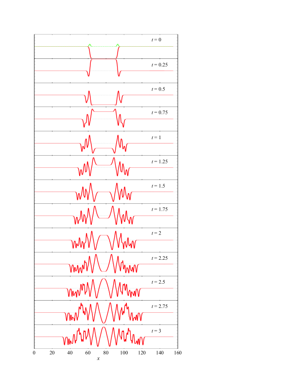
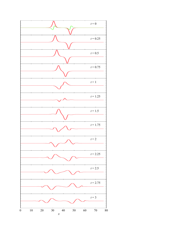
Typical scenarios are depicted in Figs. 5 and 6, for the scattering case of two kink–anti-kink waves, and two pulse–anti-pulse waves, respectively. The solution of the kink–anti-kink “scattering” waves appears to correspond to a spatially localized, persistent time-periodic oscillatory bound-state (or a breather breather1 ; breather2 ) with some radiation (phonons) at late times. Breathers are intrinsically dynamic nonlinear excitations and can be viewed as a bound state of phonons. The scattering of pulse–anti-pulse is different: there is a flip after collision and relatively less radiation.

VI Energy of solitary waves and the Peierls-Nabarro barrier

In a discrete lattice there is an energy cost associated with moving a localized mode by a half lattice constant, known as Peierls-Nabarro (PN) barrier PN ; peyrard . In the $m\rightarrow 1$ limit the elliptic functions become localized and become either pulses, or kink-like solitary waves. We shall now show that, rather remarkably, the PN barrier vanishes in this model for both types of localized modes. In fact we prove an even stronger result, that the PN barrier is zero for all three periodic solutions (in terms of ${\rm sn},{\rm cn}$ and ${\rm dn}$). If the folklore of nonzero PN barrier being indicative of non-integrability of the discrete nonlinear system is correct, then á là AL lattice, this could also be an integrable model. It would be worthwhile if one can prove this explicitly by finding the Lax pair for this model.

We start from the conserved energy expression given by Eq. (V) with $\Delta V$ of Eq. (68). First of all, we shall show that in the time-dependent as well as in the static cases, the conserved energy is given by

$$V[\phi_{n}]\sum_{n}\left[-\frac{\phi_{n+1}\phi_{n}}{\epsilon^{2}}+B\ln(1-\alpha\phi_{n}^{2})+A\right]\>,$$ (121)

where the constants A and B vary for each case. We first note that in view of Eqs. (64) and (67), we have

$$\frac{\dot{\phi}_{n}^{2}}{2(1-\alpha\phi_{n}^{2})}\ =\ -\frac{1}{2\alpha(1-\alpha\phi_{n}^{2})}\Bigl{(}a_{1}\phi_{n}^{4}+a_{2}\phi_{n}^{2}+a_{3}\Bigr{)}\>.$$ (122)

Combining this term with $\Delta V$ of Eq. (68) in the energy expression (V), we then find that the conserved energy is given by

$$E=\sum_{n}\biggl{[} \left(\frac{1}{\epsilon^{2}}-\frac{\lambda}{2\alpha}+\frac{a_{1}}{\alpha^{2}}\right)\phi_{n}^{2}-\frac{\phi_{n+1}\phi_{n}}{\epsilon^{2}}$$ (123)

$$+\frac{1}{2\alpha^{2}}\Bigl{(}a_{2}+\frac{a_{1}}{\alpha}\Bigr{)}$$

$$+\left(\frac{\lambda a^{2}}{2\alpha}-\frac{\lambda}{2\alpha^{2}}+\frac{a_{1}}{\alpha^{3}}+\frac{a_{2}}{2\alpha^{2}}\right)\ln(1-\alpha\phi_{n}^{2})\biggr{]}\>.$$

Quite remarkably we find that in the case of all the (i.e. ${\rm sn},{\rm cn}$ as well as ${\rm dn}$) solutions

$$\frac{1}{\epsilon^{2}}-\frac{\lambda}{2\alpha}+\frac{a_{1}}{\alpha^{2}}=0\>,$$ (124)

where use has been made of relevant equations in Sec. IV. As a result the $\phi_{n}^{2}$ term vanishes. Thus the conserved energy takes a rather simple form as given by Eq. (121) in the case of all of our solutions, and the constants $A$ and $B$ are given by

$$A\ =\ \frac{1}{2\alpha^{2}}\ \Bigl{(}a_{2}+\frac{a_{1}}{\alpha}\Bigr{)}\>,$$ (125)

$$B\ =\ \frac{\lambda a^{2}}{2\alpha}-\frac{\lambda}{2\alpha^{2}}+\frac{a_{1}}{\alpha^{3}}+\frac{a_{2}}{2\alpha^{2}}\>.$$ (126)

Here $a_{1},a_{2},a_{3}$ have different values for the three cases and are as given in Sec. IV. In the special case of the static solutions, there is a further simplification in that the constant term also vanishes, since $a_{1,2,3}$ are all zero in that case.

Let us now calculate the PN barrier in the case of the three periodic solutions obtained in Sec. IV and show that it vanishes in all the three cases. Before we give the details, let us explain the key argument. If we look at the conserved energy expression as given by Eq. (121), we find that there are two $c$-dependent sums involved here. We also observe that in these expressions, time $t$ and the constant $c$ always come together in the combination

$$k_{1}=\beta(c\epsilon-vt)~{}.$$ (127)

Further, using the recently discovered identities for Jacobi elliptic functions we explicitly show that for all the solutions the first sum is $c$-independent. Since the total energy $E$ as given by Eq. (121) is conserved, its value must be independent of time $t$ and since time $t$ and the constant $c$ always come together in the combination $k_{1}$ as given by Eq. (127), it then follows that the second sum must also be $c$-independent and thus there is no PN barrier for any of our periodic, and hence also the localized pulse or kink, solutions.

In particular, the following three cyclic identities khare will allow us to explicitly perform the first sum in Eq. (121):

$$m\ {\rm sn}(x)\ {\rm sn}(x+a)-\ {\rm ns}(a)$$ (128)

$$\times\ \left[Z(x+a)-Z(x)-Z(a)\right]\>,$$

$$m\ {\rm cn}(x)\ {\rm cn}(x+a)= m\ {\rm cn}(a)$$ (129)

$$+{\rm ds}(a)\left[Z(x+a)-Z(x)-Z(a)\right]\>,$$

and

$${\rm dn}(x)\ {\rm dn}(x+a)= {\rm dn}(a)$$ (130)

$$+{\rm cs}(a)\left[Z(x+a)-Z(x)-Z(a)\right]\>.$$

Here $Z(x)\equiv Z(x,m)$ is the Jacobi zeta function stegun ; byrd . In addition, we use the fact that

$$\sum_{n=1}^{N}\ \Bigl{\{}Z[\beta\epsilon(n+1)+k_{1},m]-Z(n\beta\epsilon+k_{1},m)\Bigr{\}}=0\>.$$ (131)

Let us now consider the sum as given by first term of Eq. (121) for the three cases. We first consider the kink-like solution which can also be written as

$$\phi_{n}=Aa\ {\rm sn}(n\beta\epsilon+k_{1},m)\>.$$ (132)

Using the identities given above, we obtain

$$\sum_{n=1}^{N}\left[-\frac{(\phi_{n+1}\phi_{n})}{\epsilon^{2}}\right]=-\frac{(Aa)^{2}{\rm ns}(\beta\epsilon)}{m\epsilon^{2}}\ N\ Z(\beta\epsilon)\>.$$ (133)

For the ${\rm dn}$ pulse-like case we have instead

$$\phi_{n}=Aa\ {\rm dn}(n\beta\epsilon+k_{1},m)\>,$$ (134)

and the first sum in Eq. (121) becomes

$$\sum_{n=1}^{N}\left[-\frac{\phi_{n+1}\phi_{n}}{\epsilon^{2}}\right]$$ (135)

$$=-\frac{N(Aa)^{2}}{\epsilon^{2}}\left[{\rm dn}(\beta\epsilon)-{\rm cs}(\beta\epsilon)Z(\beta\epsilon)\right]\>.$$

Finally, for the ${\rm cn}$ pulse-like case we have

$$\phi_{n}=Aa\ {\rm cn}(n\beta\epsilon+k_{1},m)\>.$$ (136)

In this case, the first sum in Eq. (121) becomes

$$-\ \sum_{n=1}^{N}\frac{\phi_{n+1}\phi_{n}}{\epsilon^{2}}=-\frac{N(Aa)^{2}}{\epsilon^{2}}\left[\frac{1}{m}Z(\beta\epsilon){\rm ds}(\beta\epsilon)-{\rm cn}(\beta\epsilon)\right]\>.$$ (137)

It is worth noting that all these sums are independent of the constant $k_{1}$ and hence $c$. As argued above, since the total energy E as given by Eq. (121) is conserved (and hence time-independent) and since $t$ and $c$ always appear together in the combination $k_{1}$ in Eq. (121) therefore it follows that the second sum in Eq. (121) must also be independent of $k_{1}$ and hence $c$. We thus have shown that the PN barrier is zero for the three periodic solutions and hence also for the localized solutions (which are obtained from them in the limit $m=1$).

In fact, it is easy to show that for all the three cases, the second sum (apart from a trivial $k_{1}$-independent constant) in Eq. (6.1) is given by

$$\sum_{n=1}^{N}\ln\left[1+\frac{{\rm sn}^{2}(\beta\epsilon)}{{\rm cn}^{2}(\beta\epsilon)}{\rm dn}^{2}(n\beta\epsilon+k_{1})\right]~{}.$$ (138)

In particular, for the solution (132) the second sum is given by

$$B\sum_{n=1}^{N}\bigg{\{}\ln[{\rm cn}^{2}(\beta\epsilon)]+\ln\left[1+\frac{{\rm sn}^{2}(\beta\epsilon)}{{\rm cn}^{2}(\beta\epsilon)}{\rm dn}^{2}(n\beta\epsilon+k_{1})\right]\bigg{\}}~{}.$$ (139)

On the other hand, for the solution (134), the second sum is given by

$$B\sum_{n=1}^{N}\ln\Bigl{[}1+\frac{{\rm sn}^{2}(\beta\epsilon)}{{\rm cn}^{2}(\beta\epsilon)}{\rm dn}^{2}(n\beta\epsilon+k_{1})\Bigr{]}~{}.$$ (140)

Finally, for the solution (136), the second sum is given by

$$B\sum_{n=1}^{N}\bigg{\{}\ln\frac{{\rm cn}^{2}(\beta\epsilon)}{{\rm dn}^{2}(\beta\epsilon)}+\ln\left[1+\frac{{\rm sn}^{2}(\beta\epsilon)}{{\rm cn}^{2}(\beta\epsilon)}{\rm dn}^{2}(n\beta\epsilon+k_{1})\right]\bigg{\}}\>.$$ (141)

It is worth remarking at this point that by following the above arguments, it is easily shown that even in the AL model AL the PN barrier is zero for the periodic ${\rm dn}$ and ${\rm cn}$ solutions. In particular, since in that case the energy is essentially given by the first sum in Eq. (121), hence using Eqs. (135) and (137) it follows that indeed for both ${\rm dn}$ and ${\rm cn}$ solutions scott there is no PN barrier in the AL model.

In general, we do not know how to write the sum in Eq. (138) in a closed form. However, for $m=1$ and $N\rightarrow\infty$, the sum of logarithms in Eq. (123) can be carried out explicitly, and the energy of the solitary wave can be given in a closed form.

We proceed as follows: One can show that, for $N\rightarrow\infty$, the following identity can be derived from the AL equation (see, for instance, Ref. cai ):

$$\sum_{n=-\infty}^{\infty}\ln\Bigl{\{}1+\sinh^{2}(\rho)\ {\rm sech}^{2}[\rho(n-x)]\Bigr{\}}\ =\ \frac{2}{\rho}\>.$$ (142)

Then, for kink-like solutions and $m=1$, we have

$$\ln(1- \alpha\phi_{n}^{2})\ln[1-\tanh^{2}(\beta\epsilon)\tanh^{2}(n\beta\epsilon+k_{1})]$$

$$=\ \ln{\rm sech}^{2}(\beta\epsilon)\ +\ \ln[1+\sinh^{2}(\beta\epsilon)\ {\rm sech}^{2}n\beta\epsilon+k_{1})]\>.$$

Thus, in the limit when $N\rightarrow\infty$ and $m=1$, the sum of logarithms in Eq. (123) becomes

$$\frac{2}{\beta\epsilon}\ +\ \sum_{n}\ \ln{\rm sech}^{2}(\beta\epsilon)\>.$$ (143)

Similarly, in the case of the two pulse solutions, ${\rm dn}$ and ${\rm cn}$ are identical for $m=1$, and we can write

$$\ln(1- \alpha\phi_{n}^{2})\ln[1+\sinh^{2}(\beta\epsilon)\ {\rm sech}^{2}(n\beta\epsilon+k_{1})]\>.$$

In the limit when $N\rightarrow\infty$, the sum of logarithms in Eq. (123) for the two pulse solutions, ${\rm dn}$ and ${\rm cn}$, for $m~{}=~{}1$, is simply equal to $2/(\beta\epsilon)$.

For the case of the kink solution, for $m=1$, $B$ as given by Eq. (126) simplifies to

$$B=-\frac{{\rm sech}^{2}(\beta\epsilon)}{\alpha\epsilon^{2}}\>,$$ (144)

whereas for the case of the pulse solutions, at $m=1$, $B$ simplifies to

$$B=-\frac{\cosh(\beta\epsilon)}{\alpha\epsilon^{2}}\>.$$ (145)

VII Conclusions

In this paper we have shown how to modify the naive discretization of $\lambda\phi^{4}$ field theory so that the discrete theory is a Hamiltonian dynamical system containing both static and moving solitary waves. We have found three different periodic elliptic solutions. For time-dependent solutions we found the unusual result that the discretization is dependent on the velocity.

In the static case, we have studied the stability of both kink-like and pulse-like solutions, and have found different qualitative behavior of the lowest eigenvalue of the stability matrix in the two cases. For typical values of the model parameters, in the case of kink-like solutions, we found that stability requires the number of sites, $N$, to be larger than a minimum value, while for pulse-like solutions stability is achieved for arbitrary values of $N$. The magnitude of the lowest eigenvalues increases with $N$ in the kink-like case, and decreases with $N$ for pulse-like solutions. The lattice spacing, $\epsilon$, is not an independent parameter and always decreases with $N$.

We also determined the energy of the solitary wave in the three cases. Using the Hamiltonian structure, we were able to argue that the PN barrier PN ; peyrard for all solitary waves is zero. This leads to the intriguing question whether this Hamiltonian system is integrable. As an additional result we explicitly showed that for the two elliptic solutions (${\rm dn}$ and ${\rm cn}$) scott of the integrable Ablowitz-Ladik model AL the PN barrier is zero–as one would expect.

The single solitary wave solutions were found to be stable and when we scattered two such single-kink solitary waves there were two different behaviors. For pulses, the pulse–anti-pulse solution leads to scattering with a flip and a little radiation (phonons). The existence of phonons brings into question the integrability of this model, in spite of the zero PN barrier. For kink-like solutions we found a breather-like behavior breather2 during the collision. However, we have not found exact two-solitary wave or breather solutions, which would help clarify the integrable nature of this system.

The results presented here are useful for structural phase transitions dphi4 ; aubry and possibly for certain field theoretic contexts luis . Our results also hold promise for appropriate discretizations of other discrete nonlinear soliton-bearing equations clark ; scott . Possible extension to discrete integrable models in $2+1$ dimensions, e.g. Kadomtsev-Petviashvili (KP) hierarchies KP , would be especially desirable. Extension to time-discrete integrable models capel is another interesting possibility.

VIII Acknowledgment

This work was supported in part by the U.S. National Science Foundation and in part by the Department of Energy. FC and BM would like to thank the Santa Fe Institute for hospitality. AK acknowledges the hospitality of the Theoretical Division at LANL where this work was initiated.

References

- (1) M. J. Ablowitz and P. A. Clarkson, Solitons, Nonlinear Evolution Equations and Inverse Scattering, (Cambridge Univ. Press, New York, 1991).
- (2) A. Scott, Nonlinear Science: Emergence & Dynamics of Coherent Structures (Oxford University Press, Oxford, 1999).
- (3) M. J. Ablowitz and J. F. Ladik, J. Math. Phys. 16, 598 (1975); ibid. 17, 1011 (1976).
- (4) M. Toda, Phys. Rep. 18c, 1 (1975); Theory of Nonlinear Lattices, M. Toda (Springer-Verlag, Berlin, 1981).
- (5) V. A. Verbus and A. P. Protogenov, Theor. Math. Phys. 119, 420 (1999).
- (6) R. Hirota, J. Phys. Soc. Jpn. 43, 2079 (1977).
- (7) S. J. Orfanidis, Phys. Rev. D 18, 3822 (1978).
- (8) P. G. Kevrekidis, K. Ø. Rasmussen, and A. R. Bishop, Int. J. Mod. Phys. B 15, 2833 (2001).
- (9) J. Ford, Phys. Rep. 213, 271 (1992); G. P. Berman and F. M. Izrailev, e-print nlin/0411062.
- (10) F. R. N. Nabarro, Theory of Crystal Dislocations (Oxford Univ. Press, London, 1967).
- (11) H. J. Mikeska, J. Phys. C 11, L29 (1978).
- (12) J. F. Weisz, J. B. Sokoloff, and J. E. Sacco, Phys. Rev. B 20, 4713 (1979).
- (13) S. Gatz and J. Herrmann, J. Opt. Soc. Am. B 8, 2296 (1991); S. Gatz and J. Herrmann, Opt. Lett. 17, 484 (1992).
- (14) H. S. Eisenberg, Y. Silberberg, R. Morandotti, A. R. Boyd, and J.S. Aitchison, Phys. Rev. Lett. 81, 3383 (1998).
- (15) A. Trombettoni and A. Smerzi, Phys. Rev. Lett. 86, 2353 (2001).
- (16) J. A. Krumhansl and J. R. Schrieffer, Phys. Rev. B 11, 3535 (1975).
- (17) L. M. A. Bettencourt, F. Cooper, and K. Pao, Phys. Rev. Lett. 89, 112301 (2002).
- (18) O. M. Braun and Yu. S. Kivshar, Phys. Rev. B 43, 1060 (1991); Yu. S. Kivshar and D. K. Campbell, Phys. Rev. E 48, 3077 (1993).
- (19) T. Dauxois and M. Peyrard, Phys. Rev. Lett. 70, 3935 (1993).
- (20) A. Khare and U. Sukhatme, J. Math. Phys. 43, 3798 (2002); A. Khare, A. Lakshminarayan, and U. Sukhatme, J. Math. Phys. 44, 1822 (2003); math-ph/0306028; Pramana (Journal of Physics) 62, 1201 (2004).
- (21) Handbook of Mathematical Functions with Formulas, Graphs, and Mathematical Tables, edited by M. Abramowitz and I. A. Stegun (U.S. GPO, Washington, D.C., 1964).
- (22) P. F. Byrd and M. D. Friedman, Handbook of Elliptic Integrals for Engineers and Scientists, 2nd ed. (Springer-Verlag, New York, 1971).
- (23) A. Khare, K. Ø. Rasmussen, M. R. Samuelsen, and A. Saxena, J. Phys. A 38, 807 (2005).
- (24) S. Aubry, J. Chem. Phys. 64, 3392 (1976).
- (25) A. Das, Integrable Models (World Scientific, Singapore, 1989).
- (26) A. C. Scott, F. Y. F. Chu, and D. W. McLaughlin, Proc. IEEE 61, 1443 (1973).
- (27) S. R. Phillpot, A. R. Bishop, and B. Horovitz, Phys. Rev. B 40, 1839 (1989).
- (28) A. Khare and U. Sukhatme, e-print math-ph/0312074; Pramana (Journal of Physics) 63, 921 (2004).
- (29) S. David Cai, Ph.D. Thesis (Northwestern University, Evanston, IL, 1994).
- (30) H. Aratyn, E. Nissimov, and S. Pacheva, Phys. Lett. B 331, 82 (1994).
- (31) F. W. Nijhoff and H. W. Capel, Phys. Lett. A 163, 49 (1992).