A method to discern complexity in two-dimensional patterns
generated by coupled map lattices

Abstract

Complex patterns generated by the time evolution of a one-dimensional digitalized coupled map lattice are quantitatively analyzed. A method for discerning complexity among the different patterns is implemented. The quantitative results indicate two zones in parameter space where the dynamics shows the most complex patterns. These zones are located on the two edges of an absorbent region where the system displays spatio-temporal intermittency.

This century has been told to be the century of complexity hawking . Nowadays the question ‘what is complexity?’ is circulating over the scientific crossroads of physics, biology, mathematics and computer science, although under the present understanding of the world there seems to be no urgency to answer the above question. However, many different points of view have been developed to this respect and hence a lot of different answers can be found, at present, in the literature perakh .

It should be kept in mind that in ancient epochs, time, space, mass, velocity, charge, color, etc. were only perceptions. Only after that they became concepts, different tools and instruments were invented for quantifying those perceptions, and, finally, only with numbers the scientific laws emerge. In this sense, if by complexity it is to be understood that property present in all systems attached under the epigraph of ‘complex systems’, this property should be reasonably quantified by the different measures that were proposed in the last years. This kind of indicators is found in those fields where the concept of information is crucial. Thus, the effective measure of complexity grassberger , the thermodynamical depth lloyd and the simple measure of complexity shiner come from physics and other attempts such as algorithmic complexity kolmogorov ; chaitin , Lempel-Ziv complexity lempel and $\epsilon$-machine complexity crutchfield arise from the field of computational sciences.

In particular, taking into account the statistical properties of a system, an indicator called the LMC (LópezRuiz-Mancini-Calbet) complexity has been introduced lopezruiz95 . This magnitude identifies the entropy or information stored in a system and its disequilibrium i.e., the distance from its actual state to the probability distribution of equilibrium, as the two basic ingredients for calculating its complexity. If $H$ denotes the information stored in the system and $D$ is its disequilibrium, the LMC complexity $C$ is given by the formula:

$$C(\{p_{i}\})=H(\{p_{i}\})\cdot D(\{p_{i}\})\;=$$

$$=-k\left(\sum_{i=1}^{N}p_{i}\log p_{i}\right)\cdot\left(\sum_{i=1}^{N}\,\left(p_{i}-\frac{1}{N}\right)^{2}\right)\,$$ (1)

where $\{p_{i}\}$, with $p_{i}\geq 0$ and $i=1,\cdots,N$, represents the distribution of the $N$ accessible states to the system, and $k$ is a constant.

As it can be straightforwardly seen, the LMC complexity vanishes both for completely ordered and for completely random systems as it is required for the correct asymptotic properties of a such well-behaved measure. Recently, it has been successfully used to discern situations regarded as complex in discrete systems out of equilibrium plastino ; calbet ; martin ; guozhang ; zuguo ; rosso .

As an example, the local transition to chaos via intermittency pomeau80 in the logistic map, $x_{n+1}=\lambda x_{n}(1-x_{n})$ presents a sharp transition when C is plotted versus the parameter $\lambda$ in the region around the instability for $\lambda\sim\lambda_{t}=3.8284$. When $\lambda<\lambda_{t}$ the system approaches the laminar regime and the bursts become more unpredictable. The complexity increases. When the point $\lambda=\lambda_{t}$ is reached a drop to zero occurs for the magnitude $C$. The system is now periodic and it has lost its complexity. The dynamical behavior of the system is finally well reflected in the magnitude $C$ (see Fig. 3a of Ref. lopezruiz95 ).

When a one-dimensional array of such maps is put together a more complex behavior can be obtained depending on the coupling among the units. Ergo the phenomenon called spatial-temporal intermittency can emerge chate87 ; chate88 ; jensen90 ; jensen98 . This dynamical regime corresponds with a situation where each unit is weakly oscillating around a laminar state that is aperiodically and strongly perturbed for a traveling burst. In this case, the plot of the one-dimensional lattice evolving in time gives rise to complex patterns on the plane. If the coupling among units is modified the system can settle down in an absorbing phase where its dynamics is trivial coullet ; toral and then homogeneous patterns are obtained. Therefore an abrupt transition to spatio-temporal intermittency can be depicted by the system pomeau86 ; sinha when modifying the coupling parameter.

In this letter we are concerned with measuring $C$ in a such transition for a coupled map lattice of logistic type. Our system will be a line of sites, $i=1,\ldots,L$, with periodic boundary conditions. In each site $i$ a local variable $x_{i}^{n}$ evolves in time ($n$) according to a discrete logistic equation. The interaction with the nearest neighbors takes place via a multiplicative coupling:

$$x_{i}^{n+1}=(4-3pX_{i}^{n})x_{i}^{n}(1-x_{i}^{n}).$$ (2)

The variable $X_{i}^{n}$ is the digitalized local mean field,

$$X_{i}^{n}=nint\left[\frac{1}{2}\>({x_{i+1}^{n}+x_{i-1}^{n}})\right]\>,$$ (3)

with $nint(.)$ the integer function rounding its argument to the nearest integer, and $p$ is the parameter of the system measuring the strength of the coupling ($0<p<1$).

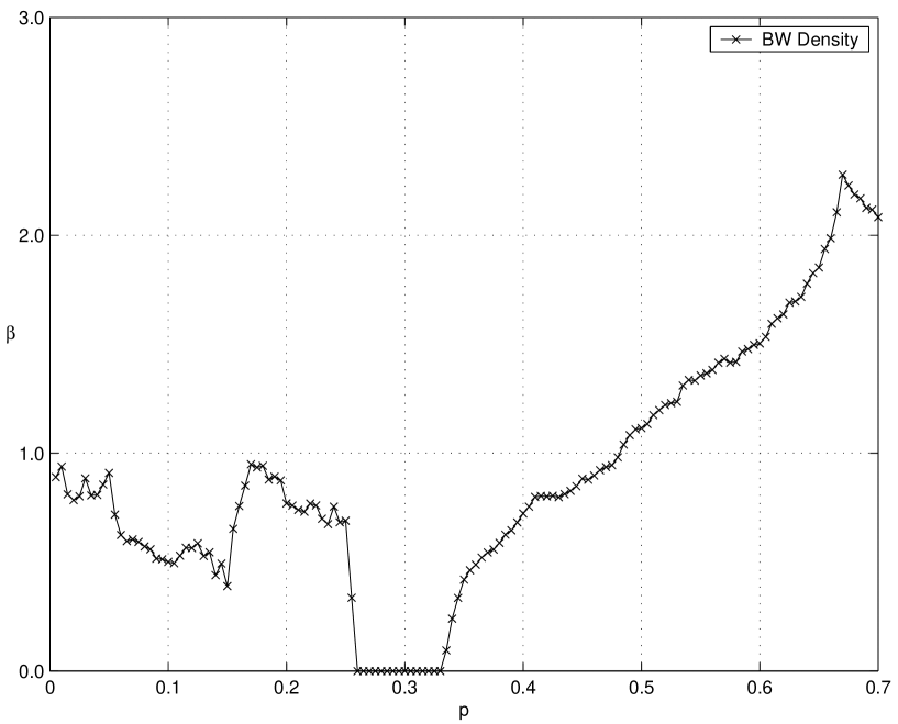
There is a biological motivation behind this kind of systems lopezruiz04 ; lopezruiz05 . It could represent a colony of interacting competitive individuals. They evolve randomly when they are independent ($p=0$). If some competitive interaction ($p>0$) among them takes place the local dynamics loses its erratic component and becomes chaotic or periodic in time depending on how populated the vicinity is. Hence, for bigger $X_{i}^{n}$ more populated is the neighborhood of the individual $i$ and more constrained is its free action. At a first sight, it would seem that some particular values of $p$ could stabilize the system. In fact, this is the case. Let us choose a number of individuals for the colony ($L=500$ for instance), let us initialize it randomly in the range $0<x_{i}<1$ and let it evolve until the stationary regime is attained. Then the black/white statistics of the system is performed. That is, the state of the variable $x_{i}$ is compared with the critical level $0.5$ for $i=1,\ldots,L$: if $x_{i}>0.5$ the site $i$ is considered white (high density cell) and a counter $N_{w}$ is increased by one, or if $x_{i}<0.5$ the site $i$ is considered black (low density cell) and a counter $N_{b}$ is increased by one. This process is executed in the stationary regime for a set of iterations. The black/white statistics is then the rate $\beta=N_{b}/N_{w}$. If $\beta$ is plotted versus the coupling parameter $p$ the Figure 1 is obtained.

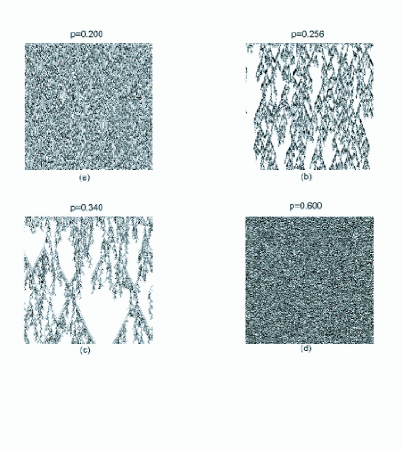
The region $0.258<p<0.335$ where $\beta$ vanishes is remarkable. As stated above, $\beta$ represents the rate between the number of black cells and the number of white cells appearing in the two-dimensional digitalized representation of the colony evolution. A whole white pattern is obtained for this range of $p$. The phenomenon of spatio-temporal intermittency is displayed by the system in the two borders of this parameter region (Fig. 2). Bursts of low density (black color) travel in an irregular way through the high density regions (white color). In this case two-dimensional complex patterns are shown by the time evolution of the system (Fig. 2b-c). If the coupling $p$ is far enough from this region, i.e., $p<0.25$ or $p>0.4$, the absorbent region loses its influence on the global dynamics and less structured and more random patterns than before are obtained (Fig. 2a-d).

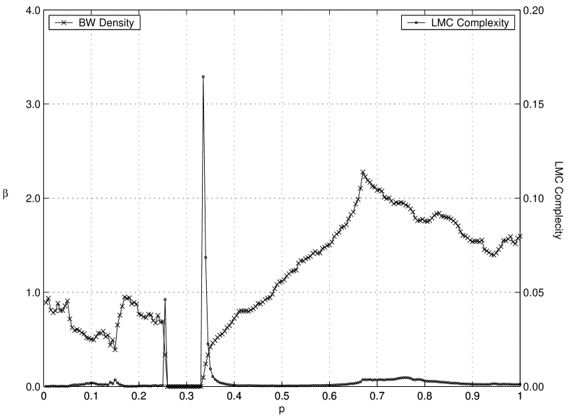
If the LMC complexity is quantified as function of $p$, our intuition is confirmed. The method proposed in Ref. lopezruiz95 to calculate $C$ is now adapted to the case of two-dimensional patterns. We let the system evolve until the stationary regime is attained. The variable $x_{i}^{n}$ in each cell is successively transformed in a binary sequence ($0$ if $x_{i}^{n}<0.5$ and $1$ if $x_{i}^{n}>0.5$) when $i$ covers the lattice, $i=1,\ldots,L$, and when $n$ is consecutively increased. This binary string is analyzed in blocks of $n_{o}$ bits, where $n_{o}$ can be considered the scale of observation. The accessible states to the system among the $2^{n_{o}}$ possible states is found as well as their probabilities. Then, the magnitudes $H$, $D$ and $C$ are directly calculated. Figure 2 shows the result for the case of $n_{o}=10$. Let us observe that the highest $C$ is reached when the dynamics displays spatio-temporal intermittency, that is, the most complex patterns are obtained for those values of $p$ that are located on the borders of the absorbent region $0.258<p<0.335$. Thus the plot of $C$ versus $p$ shows two tight peaks around the values $p=0.256$ and $p=0.34$ (Fig. 3).

If the detection of complexity in the two-dimensional case requires to identify some sharp change when comparing different patterns, those regions in the parameter space where an abrupt transition happens should be explored in order to obtain the most complex patterns. Smoothness seems not to be at the origin of complexity. As well as a selected few distinct molecules among all the possible are in the basis of life mckay , discreteness and its spiky appearance could indicate the way towards complexity. Let us recall that the distributions with the highest LMC complexity are just those distributions with a spiky-like appearance calbet . In this line, the striking result here exposed confirms the capability of the LMC complexity for signaling a transition to complex behavior when regarding two-dimensional patterns.

Acknowledgments

The authors would like to express their gratitude to Internet. It has permitted them to achieve the present transatlantic collaboration. They hope to have the possibility to shake their hands some day in the next future.

Figure 1: ($\times$) $\beta$ versus $p$. The $\beta$-statistics (or BW density) for each $p$ is the rate between the number of black and white cells depicted by the system in the two-dimensional representation of its after-transient time evolution. (Computations have been performed with $\Delta p=0.01$ for a lattice of $10000$ sites after a transient of $5000$ iterations and a running of other $5000$ iterations).

Figure 2: Digitalized plot of the one-dimensional coupled map lattice (axe OX) evolving in time (axe OY) according to Eq. (2): if $x_{i}^{n}>0.5$ the $(i,n)$-cell is put in white color and if $x_{i}^{n}<0.5$ the $(i,n)$-cell is put in black color. The discrete time $n$ is reset to zero after the transitory. (Lattices of $300\times 300$ sites, i.e., $0<i<300$ and $0<n<300$).

Figure 3: ($\Box$) $C$ versus $p$. Observe the peaks of the LMC complexity located just on the borders of the absorbent region $0.258<p<0.335$, where $\beta=0$ ($\times$). (Computations have been performed with $\Delta p=0.01$ for a lattice of $10000$ sites after a transient of $5000$ iterations and a running of other $5000$ iterations).

References

- (1) “I think the next century will be the century of complexity”, Stephen Hawking (2000).
- (2) M. Perakh,“Defining complexity”, On Talk Reason, www.talkreason.org/articles/complexity.pdf, August (2004).
- (3) P. Grassberger, Int. J. Theor. Phys. 25, 907 (1986).
- (4) S. Lloyd and H. Pagels, Ann. Phys. (NY) 188, 186 (1988).
- (5) J.S. Shiner, M. Davison and P.T. Landsberg, Phys. Rev. E 59, 1459 (1999).
- (6) A.N. Kolmogorov, Probl. Inform. Theory 1, 3 (1965).
- (7) G. Chaitin, J. Assoc. Comput. Mach. 13, 547 (1966).
- (8) A. Lempel and J. Ziv, IEEE Trans. Inform. Theory 22, 75 (1976).
- (9) J.P. Crutchfield and K. Young, Phys. Rev. Lett. 63, 105 (1989).
- (10) R. López-Ruiz, H.L. Mancini and X. Calbet, Phys. Lett. A 209, 321 (1995).
- (11) C.Anteneodo and A.R. Plastino, Phys. Lett. A 223, 348 (1996).
- (12) X. Calbet and R. López-Ruiz, Phys. Rev. E 6, 066116(9) (2001).
- (13) M.T. Martin, A. Plastino and O.A. Rosso, Phys. Lett. A 311 (2-3), 126 (2003).
- (14) G. Feng and S. Song and P. Li, J. Hydr. Eng. Chin. (Hydr. Eng. Soc.) 11, article no. 14 (1998).
- (15) Z. Yu and G. Chen, Comm. Theor. Phys. (Beijing China) 33 673 (2000).
- (16) O.A. Rosso, M.T. Martin and A. Plastino, Physica A 320, 497 (2003).
- (17) Y. Pomeau and P. Manneville, Commun. Math. Phys. 74, 189 (1980).
- (18) H. Chaté and P. Manneville, Phys. Rev. Lett. 58, 112 (1987).
- (19) H. Chaté and P. Manneville, Phys. Rev. A 38, 4351 (1988).
- (20) J.M. Houlrik, I. Webman and M.H. Jensen, Phys. Rev. A 41, 4210 (1990).
- (21) J. Rolf, T. Bohr and M.H. Jensen, Phys. Rev. E 57, R2503 (1998).
- (22) M. Argentina and P. Coullet, Phys. Rev. E 56, R2359 (1997).
- (23) M.G. Zimmermann, R. Toral, O. Piro and M. San Miguel, Phys. Rev. Lett. 85, 3612 (2000).
- (24) Y. Pomeau, Physica D 23, 3 (1986).
- (25) G.I. Menon, S. Sinha and P. Ray, Europhys. Lett. 61, 27 (2003).
- (26) R. López-Ruiz and D. Fournier-Prunaret, Math. Biosc. Eng. 1, 307 (2004).
- (27) R. López-Ruiz and D. Fournier-Prunaret, preprint nlin.AO/0406020 or also in the abstracts of the conference ‘Verhulst 200 on Chaos’, p. 56, Royal Military Academy, Brussels (2004 ).
- (28) C.P. McKay, “What is life?”, PLOS Biology 2, 1260 (2004).