Planar dimers and Harnack curves

1 Introduction

1.1 Summary of results

In this paper we study the connection between dimers and Harnack curves discovered in [15]. To any periodic edge-weighted planar bipartite graph $\Gamma$ one associates its spectral curve $P(z,w)=0$. The real polynomial $P$ defining the spectral curve arises as the characteristic polynomial of the Kasteleyn operator in the dimer model.

It was shown in [15] that for real positive edge weights on $\Gamma$ the curves thus obtained are real curves of a very special kind, namely they are Harnack curves. Harnack curves are, in some sense, the best possible real plane curves. They were studied both classically and recently, see [16, 17] and references therein. Here we prove that every Harnack curve arises as a spectral curve of some dimer model. This gives a parameterization of the set of Harnack curves which, in spirit, is similar to the classical parametrization of totally positive matrices. It may be compared with the result of Vinnikov [21] who gave a similar description of real plane curves with a maximally nested set of ovals (which form a class of curves in some sense opposite to Harnack curves).

We also prove that modulo the natural $(\mathbb{R}^{\times})^{2}$-action the set of degree $d$ Harnack curves in $\mathbb{P}^{2}(\mathbb{R})$ is diffeomorphic to the closed octant $\mathbb{R}_{\geq 0}^{(d+4)(d-1)/2}$. In fact, the areas of the amoeba holes and the distances between the amoeba tentacles give these global coordinates.

The Kasteleyn operator of the dimer model is an example of a periodic finite-difference operator (weighted adjacency matrix of a periodic graph). The spectral theory of such operators is much developed, stimulated, in particular, by their connections with integrable systems, see, for example, [2, 6, 9] for an introduction. The particular type of operators we consider was studied by A. Oblomkov [18] and in a series of paper by I. Dynnikov and S. Novikov [7, 8]. The spectral data associated to a periodic finite-difference operator is, typically, an algebraic variety (a curve $C$, in our case) together with a line bundle on it, that is, a together with a point of the Jacobian $J(C)$. With complex coefficients, it is usually easy to see (see e.g. [5]) that the “spectral transform”, from the operator to its spectral data, is dominating, but not surjective. Reality issues are typically more subtle. From the probabilistic origin of our spectral problem, it is natural to consider real and positive coefficients (edge weights). This adds a new aspect to the problem.

The Harnack curves of genus zero play a special role. We characterize them as the spectral curves of isoradial dimers studied in [14], see Section 5, and also as those Harnack curves that minimize the volume under their Ronkin function (with given boundary conditions), see Proposition 9. Translated into the language of probability, this means that isoradial dimer weights maximize the partition function with given boundary conditions.

1.2 Acknowledgments

This research was started at the Institut Henri Poincaré and completed while R. K. was visiting Princeton University. A. O. was partially supported by DMS-0096246 and a fellowship from Packard foundation.

2 Background

2.1 Kasteleyn operator and its spectral curve

2.1.1

Let $\Gamma$ be a periodic planar bipartite graph. We can assume that $\Gamma$ is embedded in the plane $\mathbb{R}^{2}$ in such a way that translations by the standard lattice $\mathbb{Z}^{2}$ preserve $\Gamma$, including the partition of its vertices into black and white ones. Throughout this paper, we assume that the quotient $\Gamma/\mathbb{Z}^{2}$ is finite. Let the edges of $\Gamma$ be weighted in a $\mathbb{Z}^{2}$–invariant way.

A perfect matching (also known as a dimer configuration) of a graph is a collection of edges that cover every vertex exactly once. The weight of such a matching is defined to be the product of the edge weights. Kasteleyn in [12] computed the weighted number of perfect matchings of any finite bipartite planar graph $\Gamma_{0}$ using the determinant of what is now called the Kasteleyn operator

$$\mathsf{K}:\mathbb{C}^{\textup{black vertices}}\to\mathbb{C}^{\textup{white vertices}}\,,$$ (2.1)

which is the weighted adjacency matrix of $\Gamma_{0}$ sign-twisted in a certain way, see [13] for an introduction.

The study of perfect matchings (also known as the dimer model) on infinite periodic planar graphs $\Gamma$ stimulates the study of the corresponding Kasteleyn operators, see for example [15] for further information. In this paper, we will focus on the case when $\Gamma$ is the hexagonal lattice, in which case $\mathsf{K}$ is simply the weighted adjacency matrix. This case is, in fact, universal as will be explained in Section 2.1.4.

2.1.2

The operator $\mathsf{K}$ commutes with the translation action of $\mathbb{Z}^{2}$ and, in particular, it preserves the $\mathbb{Z}^{2}$–eigenspaces. These eigenspaces are indexed by characters of $\mathbb{Z}^{2}$, that is, by a pair of Bloch-Floquet multipliers $(z,w)\in(\mathbb{C}^{*})^{2}$. They are finite–dimensional with a distinguished basis $\{\delta_{v}\}$ consisting of functions supported on a single $\mathbb{Z}^{2}$–orbit and taking value $1$ on a vertex $v$ inside a fixed fundamental domain. Let $\mathsf{K}(z,w)$ be the matrix of $\mathsf{K}$ in the basis $\{\delta_{v}\}$ and acting on the $(z,w)$-eigenspace of $\mathbb{Z}^{2}$ and set, by definition,

$$P(z,w)=\det\mathsf{K}(z,w)\,.$$ (2.2)

Different choices of the fundamental domain lead to polynomials that differ by a factor of the form $z^{i}w^{j}$. In particular, the zero locus of $P$

$$\{P(z,w)=0\}\subset(\mathbb{C}^{*})^{2}$$ (2.3)

is defined canonically and is called the spectral curve of the dimer problem.

The spectral curve remains the same if we multiply the weights of all edges incident to a given vertex by the same number. This is a gauge transformations of the dimer problem; it does not change probabilities of configurations.

The map from the weights modulo gauge to the corresponding spectral curves is our main object of study in this paper.

2.1.3

For example, for the hexagonal lattice with $d\times d$-fundamental domain, $P(z,w)$ is the determinant of the $d^{2}\times d^{2}$ matrix the construction of which is illustrated in Figure 1. We denote the weights of the 3 edges incident to a white vertex $v$ by $a_{v}$, $b_{v}$, and $c_{v}$. The dashed line in Figure 1 is the boundary of the fundamental domain. An edge crossing it is weighted by an extra factor of $z$ or $w$.

Figure 1: The operator $\mathsf{K}(z,w)$

It is clear that in this case $P(z,w)$ is polynomial in $z$ and $w$ of degree at most $d$ in each variable. In fact $P$ has total degree $d$: this can be seen by splitting the fundamental domain in half into two equilateral triangular arrays of vertices; the upper right triangle has $d$ more white vertices than black vertices so exactly $d$ edges connect this part with the rest of the graph.

2.1.4

The case of the hexagonal lattice is universal in the following sense. By choosing $d$ large enough and setting some edge weights to zero, one can produce a graph which is equivalent to an arbitrary planar periodic bipartite graph, in the following sense.

We consider two graphs to be equivalent if one can be obtained from another by a sequence of moves of the following type: remove a $1$–valent vertex and its neighbor, or remove a $2$–valent vertex, gluing its neighbors into a single vertex and redistributing the edge weights accordingly. See [19]. It is easy to see that such transformation induce a weight-preserving bijection of sets of dimer configurations.

Because of this universality we will focus in this paper on the case of hexagonal lattice with $d\times d$-fundamental domain. In this case, the spectral curve is a degree $d$ curve in the projective plane $\mathbb{P}^{2}$.

2.2 Harnack curves

2.2.1 Topological configuration of ovals

A real algebraic curve $C(\mathbb{R})\subset\mathbb{P}^{2}(\mathbb{R})$ is called an $M$-curve if it has the maximal possible number of connected components, namely $1+(d-1)(d-2)/2$, where $d$ is the degree of $C$. For brevity, we will call all these components ovals, even though this is at odds with the classical distinction between separating and nonseparating components of $C(\mathbb{R})$ (which will play no role in this paper). We will also treat isolated real points as degenerate ovals. Ovals not intersecting the coordinate axes will be called compact ovals.

Among the $M$-curves, the Harnack curves are distinguished by the position of their ovals with respect to the each other and the three coordinate lines in $\mathbb{P}^{2}$ (they are also sometimes called simple Harnack curves in the literature). The classical definition of a Harnack curve is somewhat complicated, see [16]. We will use instead modern characterizations of Harnack curves obtained in [16, 17]. By the main result of [16], for given degree $d$, a curve is a Harnack curve if and only if the topological configuration of ovals is as illustrated in Figure 2. (It is different for odd and even degree.) The numbers of ovals in each quadrant are consecutive triangular numbers. Of course, Figure 2 is only meant to illustrate the topology and not be a plot of an actual Harnack curve.

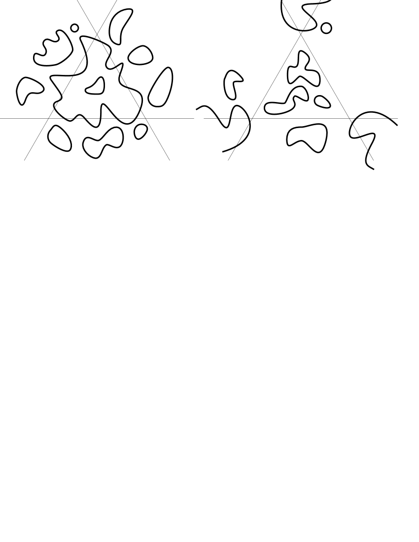
Figure 2: Oval configuration of Harnack curves of degrees $6$ and $5$

The group $(\mathbb{R}^{\times})^{2}$ acts freely on the set of Harnack curves by rescaling the variables. We will call the quotient of this action the moduli space of Harnack curves. We will see that the moduli space of degree $d$ Harnack curves is diffeomorphic to the closed octant $\mathbb{R}_{\geq 0}^{(d+4)(d-1)/2}$, in particular, it is connected and simply connected. It follows that the set of all Harnack curves has 4 connected components, corresponding to a choice of one of 4 quadrants in Figure 2. These choices are related by reversing the signs of $z$ or $w$.

There is a corresponding flexibility on the dimer problem side: rescaling $z$ and $w$ corresponds to a natural operation on dimer weights which was called changing magnetic field in [15]. From many points of view, it is natural to view this operation as a generalized gauge transformation. For example, with such extended definition of gauge equivalence, any dimer model whose spectral curve is rational is equivalent to an isoradial dimer, see Section 5.

2.2.2 Amoeba map

Another useful characterization of Harnack curves $C$ is that the map

$$(\mathbb{C}^{*})^{2}\supset C(\mathbb{C})\owns(z,w)\mapsto(\log|z|,\log|w|)\in\mathcal{A}(C)\subset\mathbb{R}^{2}$$

from the curve $C$ to its amoeba $\mathcal{A}(C)$ is generically 2-to-1 over the interior of $\mathcal{A}(C)$ (that is, 2-to-1 except at real nodes).

The (geometric) genus $g$ of a Harnack curve is the number of compact ovals that are not reduced to points. In particular, the amoeba of a genus $g$ Harnack curve has exactly $g$ compact holes, which is illustrated in Figure 5 for the case $g=3$.

The 2-to-1 property constrains the possible singularities that $C$ can have by constraining the possible links of the singular points. It was shown in [17] that the only possible degenerations of Harnack curves with fixed Newton polygon occur when some of the ovals shrink to zero size, producing real isolated double points (real nodes). In particular, it is impossible for two ovals of $C$ to meet.

2.2.3 Ronkin function and Monge-Ampère equation

A third characterization of Harnack curves $C$, obtained in [17] is by maximality of the area of their amoeba $\mathcal{A}(C)$. Concretely, $C$ is Harnack if and only if its amoeba has the maximal possible area for given Newton polygon $\Delta$, namely $\pi^{2}$ times the area of $\Delta$.

This maximality of the area is a consequence of the following Monge-Ampère equation (see [17])

$$\det\begin{pmatrix}R_{xx}&R_{xy}\\ R_{yx}&R_{yy}\end{pmatrix}=\frac{1}{\pi^{2}}\,,$$ (2.4)

satisfied for all $(x,y)$ in the interior of the amoeba $\mathcal{A}(C)$. Here $R(x,y)$ is the Ronkin function of $C$ defined by

$$R(x,y)=\frac{1}{(2\pi i)^{2}}\iint_{\begin{subarray}{c}|z|=e^{x}\\ |w|=e^{y}\end{subarray}}\,\log|P(z,w)|\,\,\frac{dz}{z}\frac{dw}{w}\,.$$ (2.5)

2.2.4 Holomorphic differentials

Holomorphic differentials on $C$ will play an important role in our analysis. In this section we recall some basic facts about them.

Suppose that $C$ has geometric genus $g$. Let $\alpha_{1},\dots,\alpha_{g}$ be the compact real ovals of $C$ that are not reduced to points, and let $\{q_{i}\}$, $i=1,\dots,\binom{d-1}{2}-g$ denote its isolated real nodes. The ovals $\alpha_{i}$ form a set of $a$-cycles in $H_{1}(C)$. The corresponding $b$-cycles can be taken in the form

$$\beta_{i}=\{|z|=e^{x_{i}},|w|<e^{y_{i}}\}\cap C$$ (2.6)

where $(x_{i},y_{i})$ is a point inside the $i$th hole of the amoeba $\mathcal{A}(C)$. The cycles $\beta_{i}$ are anti-invariant with the respect to the complex conjugation.

Holomorphic differentials on $C$ have the form

$$\omega=\frac{Q(z,w)}{\frac{\partial}{\partial w}P(z,w)}\,dz\,,$$ (2.7)

where $Q$ is a polynomial of degree $d-3$ vanishing at the points $\{q_{i}\}$, see [1]. It is a fundamental fact about plane curves (see [1], Appendix A) that the nodes $\{q_{i}\}$ impose independent conditions on polynomials of degree $d-3$. In particular, the space of differentials (2.7) is $g$-dimensional. We choose a basis $\{\omega_{i}\}$ such that

$$\int_{\alpha_{i}}\omega_{j}=\delta_{ij}\,.$$ (2.8)

The polynomials $Q_{i}$ are real and their $b$-periods are purely imaginary (since $\beta_{i}$ is anti-invariant under complex conjugation).

The polynomial $Q_{i}$ has at least two zeros on every compact oval except the $i$th, by the integral condition (2.8): the form $dz/P_{w}$ is real and of constant sign on every oval, so $Q_{i}$ must change sign at least twice on each oval except the $i$th. This implies that $Q_{i}$ must have no zeros on the $i$-th oval and precisely 2 zeros on any other oval, otherwise, the degree $d-3$ curve $Q_{i}=0$ would intersect $C$ at

$$(d-1)(d-2)>d(d-3)$$

points. It follows that the function

$$x\mapsto\int_{x_{0}}^{x}\omega_{i}\,,$$ (2.9)

where $x_{0}$ and $x$ are points on the $i$th oval, is increasing and provides a natural parametrization of the $i$th oval.

Let us call a degree $\binom{d-1}{2}$ divisor $D$ a standard divisor if it has precisely one point on each compact oval of $C$ (including degenerate ovals). By monotonicity of (2.9), the product of compact ovals of $C$, which is the variety parameterizing standard divisors, injects into the Jacobian $J(C)$ of degree $\binom{d-1}{2}$. It forms a component of its real locus.

3 The spectral problem

3.1 Boundary of the spectral curve

By the boundary of a spectral curve $C$ we mean the $3d$ points (counting multiplicity) of its intersection with the coordinate lines of $\mathbb{P}^{2}$. We show in this section that these points have a simple interpretation in terms of the weights of the dimer problem. In particular, they are real for real edge weights.

It is useful to introduce the curve $\widetilde{C}$ defined by the equation

$$\widetilde{P}(z,w)=P(z^{d},w^{d})\,.$$ (3.1)

This is a $d^{2}$-fold covering of the spectral curve $C$ ramified over its boundary. The advantage of going to this branched covering is that operator $\mathsf{K}(z^{d},w^{d})$ is gauge equivalent to the operator $\widetilde{\mathsf{K}}(z,w)$ defined by the rule illustrated in Figure 3. In the operator $\widetilde{\mathsf{K}}(z,w)$, the weights of all vertical edges are multiplied by $w$ and weights of all northwest-southeast edges are multiplied by $z$.

Figure 3: The operator $\widetilde{\mathsf{K}}(z,w)$

In particular, if $w=0$ then this operator becomes block-diagonal with blocks corresponding to chains of vertices of the form shown in Figure 4.

Figure 4: The operator $\widetilde{\mathsf{K}}(z,0)$

The determinant of the corresponding block equals

$$\det\begin{pmatrix}c_{1}&za_{2}&&\\ &c_{2}&za_{3}\\ &&c_{3}&\ddots\\ za_{d}&&&\ddots\end{pmatrix}=\prod c_{i}+(-1)^{d+1}z^{d}\prod a_{i}\,.$$ (3.2)

Therefore, the spectral curve $P(z,w)=0$ intersects the $w=0$ line at the points of the form

$$z=(-1)^{d}\prod_{\textup{$v$ in a zig-zag cycle}}c_{v}/a_{v}\,,$$ (3.3)

where by a zig-zag cycle we mean a “horizontal” chain of vertices like in Figure 4.

The alternating products of the from (3.3) taken for all paths of all 3 orientations multiply to $1$. This is, in fact, a general constraint for the boundary points of any degree $d$ curve. It can be viewed, for example, as coming from the divisor class group of the union of the coordinate lines.

Note that once the fundamental domain is fixed, we get a canonical ordering of the boundary points of the spectral curve. It comes from the ordering of the corresponding zig-zag cycles.

3.2 The divisor of a vertex

By definition, the spectral curve (2.3) is where the kernel and the cokernel of the matrix $\mathsf{K}(z,w)$ become nontrivial. For smooth spectral curves $C$, the kernel and the cokernel are $1$-dimensional [5] and form a line bundle over $C$. In particular, for every white vertex $v\in\Gamma$ the image of the function $\delta_{v}$ in

$$\operatorname{Coker}\mathsf{K}(z,w)=\mathbb{C}^{\textup{white vertices}}/\operatorname{Img}\mathsf{K}(z,w)$$

defines a section of the cokernel bundle. We will denote by $(v)$ the divisor of this section excluding the points on the boundary.

In down to earth terms, equations of $(v)$ are the cofactors of the entries of $\mathsf{K}(z,w)$ in the row corresponding to the white vertex $v$. Since the columns of $\mathsf{K}(z,w)$ are linearly dependent on the curve $C$, $(v)$ is defined locally by the vanishing of a single minor.

Theorem 1.

For real positive edge weights, the spectral curve $P(z,w)=0$ is a Harnack curve of degree $d$, in particular, it has $\binom{d-1}{2}$ compact ovals. The divisor $(v)$ of any vertex $v$ is a standard divisor on this curve.

The first part of this theorem is one of the main results of [15]. The argument given below provides a new proof of it.

Proof.

It suffices to consider the case of generic edge weights, since the properties of being a Harnack curve and being a standard divisor are closed.

Let us consider the bundle $\mathcal{L}$ formed by the cokernels of the matrix $\widetilde{\mathsf{K}}(z,w)$ on the curve $\widetilde{C}$ defined by the equation (3.1). It fits into the following exact sequence

$$0\to\mathcal{O}(-1)^{d^{2}}\xrightarrow{\,\,\widetilde{\mathsf{K}}\,\,}\mathcal{O}^{d^{2}}\to\mathcal{L}\to 0$$ (3.4)

of sheaves on $\mathbb{P}^{2}$. It follows that

$$\chi(\mathcal{L})=d^{2}\,.$$

The curve $\widetilde{C}$ has genus $(d^{2}-1)(d^{2}-2)/2$ and, therefore, by Riemann-Roch we obtain

$$\deg\mathcal{L}=\frac{d^{2}(d^{2}-1)}{2}\,.$$

Let $v$ be a white vertex and consider the section $s_{v}$ of $\mathcal{L}$ defined by the function $\delta_{v}$. The divisor of $s_{v}$ is the pull-back of $(v)$ except for the boundary contribution, which we will now determine.

Let $p$ be a boundary point of $\widetilde{C}$ corresponding to a zig-zag cycle as in Figure 4 and suppose that the vertex $v$ is $k$ steps above this path. Below we prove the following:

Lemma 1.

The order of the vanishing of $s_{v}$ at the point $p$ equals $k$.

Since every path gives rise to $d$ points on the boundary of $\widetilde{C}$, it follows that the total contribution of the boundary points to the degree of $s_{v}$ equals $3d^{2}(d-1)/2$. Subtracting it, we obtain

$$\deg(v)=\frac{1}{d^{2}}(\deg\mathcal{L}-\deg s_{v})=\frac{(d-1)(d-2)}{2}\,.$$ (3.5)

The remainder of the proof is based on the deformation to the constant weight case. If all edge weights are equal to one, the polynomial $\widetilde{P}$ takes a particularly simple form (see [15])

$$\widetilde{P}(z,w)=\prod_{i,j=1}^{d}(\varepsilon^{i}\,z+\varepsilon^{j}\,w+1)\,,$$ (3.6)

where $\varepsilon$ is a primitive $d$th root of unity. In particular, the spectral curve $C$ is a genus $0$ curve with $\binom{d-1}{2}$ isolated real nodes (isolated real solutions to $\varepsilon^{i}\,z+\varepsilon^{j}\,w+1=0$ exist when $i\neq j$ and $i,j\neq d$; moreover replacing $i,j$ with $-i,-j$ gives an identical solution). It also intersects each coordinate line once with multiplicity $d$, and, hence, satisfies the topological definition of a Harnack curve.

The space

$$\operatorname{Ker}\mathsf{K}^{*}(z,w)=\left(\operatorname{Coker}\mathsf{K}(z,w)\right)^{*}$$

is $2$-dimensional if $(z,w)$ is one of the nodes of $C$. In particular, there exists an nonzero element of this space which annihilates $\delta_{v}$. By continuity, for all nearby curves the divisor $(v)$ has a nearby point, possibly complex. By (3.5) the total number of such points equals the degree of $(v)$, hence all of them are simple real zeros (no point can bifurcate into a complex conjugate pair of zeros).

It follows that under a small real perturbation of weights, the spectral curve remains a Harnack curve and $(v)$ remains a standard divisor. Because the ovals of a Harnack curve cannot meet (see Section 2.2.2) and the boundary points do not become complex (see Section 3.1), the same statement holds globally for real positive weights.

∎

Proof of Lemma 1.

Let $(z_{0},0)$ be the coordinates of the point $p$. Note that if the corresponding intersection of the curve $C$ with the $w=0$ axes was transverse (which happens generically) then $w$ is a local parameter on $\widetilde{C}$ near $p$ and $z-z_{0}=O(w^{d})$. Therefore, near $p$ we have

$$\mathsf{K}\big{|}_{\widetilde{C}}=\begin{pmatrix}K_{1}&wB_{1}\\ &K_{2}&wB_{2}\\ &&\ddots&\ddots\\ wB_{d}&&&K_{d}\end{pmatrix}+O(w^{d})\,,$$

where the blocks $K_{i}$ correspond to zig-zag paths as in (3.2) and $B_{i}$ are diagonal invertible matrices. The matrix $K_{1}$ has a one-dimensional kernel while all other $K_{i}$’s are invertible. Clearly,

$$\operatorname{Ker}\mathsf{K}^{*}=(v,-wK_{2}^{-1}B_{1}v,w^{2}K_{3}^{-1}B_{2}K_{2}^{-1}B_{1}v,\dots)+O(w^{d})\,,$$

where $v\in\operatorname{Ker}K_{1}^{*}$. Since the entries of $\operatorname{Ker}\mathsf{K}^{*}$ are the cofactors of $\mathsf{K}$ that we need, the lemma follows. ∎

3.3 Spectral transform

We have constructed the following correspondence

$$\left(\begin{gathered}\textup{edge weights}\big{/}\textup{gauge}\\ \textup{fundamental domain}\\ \textup{vertex}\end{gathered}\right)\quad\Rightarrow\quad\left(\begin{gathered}\textup{Harnack curve}\\ \textup{ordering of boundary points}\\ \textup{standard divisor}\end{gathered}\right)\,,$$ (3.7)

which we will call the spectral transform. Our first result about it is the following

Theorem 2.

The spectral transform is injective.

Proof.

The spectral data determines the sheaf $\mathcal{L}$ introduced in the proof of Theorem 1 up to isomorphism. By Theorem 1.1 in [5], this determines the matrix $\widetilde{\mathsf{K}}(z,w)$ up to multiplication on the left and on the right by elements of $GL(d^{2},\mathbb{R})$, that is, up to a choice of linear basis of both spaces in (2.1).

Let $p$ be a boundary point of the spectral curve. It determines a filtration on the space $\mathbb{C}^{\textup{white vertices}}$ by the order of the vanishing of the corresponding section of the cokernel bundle at $p$. It is easy to see that the basis $\{\delta_{v}\}$ is the unique, up to normalization, basis compatible with all these filtrations. Same argument applied to transpose matrix $\widetilde{\mathsf{K}}^{*}$, which has the same spectral curve, reconstructs the delta-function basis of $\mathbb{C}^{\textup{black vertices}}$. As a result we reconstruct the matrix $\widetilde{\mathsf{K}}(z,w)$ up to a multiplication on the left and on the right by a diagonal matrix, that is, up to a gauge transformation. ∎

A very useful (and well-known, cf. [3, 10, 11, 20]) way of thinking about the spectral data in (3.7) is the following. The divisor is an ordered collection of distinct points of $\mathbb{P}^{2}$; similarly, the boundary points are an ordered collection of points on the coordinate axes. The spectral curve $P(z,w)$ is determined by this data as the unique degree $d$ curve passing through all these points. Indeed, since the boundary points are fixed, any other curve passing through the same points is given by

$$P(z,w)+zwQ(z,w)=0\,,\quad\deg Q\leq d-3\,.$$

But then, as in Section 2.2.4, $Q=0$ and $P=0$ will have $(d-1)(d-2)$ points in common, which is one too many.

It is clear from this description that the spectral data is parametrized by an open subset of $\mathbb{R}^{d^{2}+1}$ (which, in fact, is homeomorphic to $\mathbb{R}^{d^{2}+1}$, as we will see later). Also, this picture continues to work in a complex neighborhood and the injectivity remains valid with the same proof. It follows at once that:

Corollary 2.

The differential of the spectral transform is injective.

3.4 Surjectivity of the spectral transform

This reconstruction procedure given in Theorem 2 can be made explicit to a certain degree, but it appears to be difficult to establish the surjectivity of the spectral transform directly. Instead, we will take a different route based on the following

Proposition 3.

The spectral transform is proper.

In fact, at several points in the paper we will resort to proving surjectivity by combining properness with injectivity of the differential.

Proof.

Suppose that the spectral curve $C$ varies in some bounded set of Harnack curves. In particular, the the coefficients of $1$, $z^{d}$, and $w^{d}$ in the equation of $C$ are bounded from above and below in absolute value. Without loss of generality, we can assume that these coefficients are equal to $\pm 1$. This means that the weights of the 3 frozen matchings (matchings using all edges of the same orientation) are equal to 1. Other coefficients of $P(z,w)$, which enumerate other periodic matchings, are bounded from above in absolute value. This implies that the weight of any periodic matching is bounded from above.

Periodic matchings are the vertices of the periodic flow polytope. This polytope is formed by nonnegative periodic flows from white vertices to black vertices such that the total flux is $1$ at each black vertex. The logarithm of the weight of a matching extends as a bounded linear function to the interior of this polytope (recall that the weight of a matching is the product of its edge weights). The barycenter of this polytope is the flow of intensity $1/3$ along each edge. It has weight $1$ by our assumption.

Coordinates on the space of weights modulo gauge are given by the combinations of the form

$$\prod_{i=1}^{k}\frac{\operatorname{weight}(e_{2i-1})}{\operatorname{weight}(e_{2i})}$$ (3.8)

where $e_{1},e_{2},\dots,e_{2k}$ is a closed loop of edges on the torus, such as for example the loop in Figure 4. Such loops can be thought of as flows with zero flux. If the weight (3.8) of any such loop under the variation is unbounded, we can add a small multiple of it to the constant $1/3$ flow and obtain a point inside the periodic flow polytope with unbounded weight. This contradiction completes the proof. ∎

We will prove in Theorem 5 that the spectral data on the left in (3.7) forms a manifold diffeomorphic to $\mathbb{R}^{d^{2}+1}$. From the description (3.8) of the coordinates on the space of weights modulo gauge, it it clear that this is also diffeomorphic to $\mathbb{R}^{d^{2}+1}$. Indeed, the cycle space is $d^{2}+1$-dimensional, generated by the $d^{2}$ faces in a fundamental domain (subject to one relation), and the horizontal and vertical cycles. Therefore, we obtain

Theorem 3.

The spectral transform is a bijection.

4 The space of Harnack curves

4.1 Harnack curves of genus zero

Harnack curves of genus zero can be understood explicitly. By general theory, any real degree $d$ genus zero curve $C$ has a parametrization of the form

$$z(t)=a_{0}\,\prod_{i=1}^{d}\frac{t-a_{i}}{t-c_{i}}\,,\quad w(t)=b_{0}\,\prod_{i=1}^{d}\frac{t-b_{i}}{t-c_{i}}\,,$$ (4.1)

where $t\in\mathbb{R}P^{1}=\mathbb{R}\cup\{\infty\}$, $a_{0}$ and $b_{0}$ are nonzero real numbers, and the other parameters are either real or appear in complex conjugate pairs. Such representation is unique up to the action of $PGL_{2}(\mathbb{R})$ by fractional linear transformation of the variable $t$.

The action of $PGL_{2}(\mathbb{R})$ can by reduced down to the action of the connected group $PSL_{2}(\mathbb{R})$ once we fix the orientation of the curve $C$. We will fix some cyclic ordering of the coordinate axes and require that the $C$ intersects them in that order (see Section 2.2.1). Let the cyclic order be: $\{z=0\}$, $\{w=0\}$, and the line at infinity.

Proposition 4.

The curve (4.1) is Harnack if and only if the parameters in (4.1) are real and cyclically ordered on $\mathbb{R}P^{1}$ as follows:

$$a_{1}\leq a_{2}\leq\dots\leq a_{d}<b_{1}\leq\dots\leq b_{d}<c_{1}\leq\dots\leq c_{d}<a_{1}\,.$$ (4.2)

Proof.

In one direction, this is a part of the topological definition of the Harnack curve, see [16], which requires the curve $C$ to first intersect the line $\{z=0\}$ $d$ times, then the line $\{w=0\}$ also $d$ times, and, finally, the line at infinity $d$ times.

In the other direction, we have to show that as long as the parameters (4.2) are cyclically ordered the curve $C$ remains Harnack. Note that the strict inequalities in (4.2) ensure that $C$ doesn’t pass through the intersections of the coordinate axes, which in other words means that the Newton polygon of its equation remains the full triangle. Since the real nodes of the curve cannot disappear or merge by the $2$-to-$1$ property (see Section 2.2.2), and the region in the parameter space defined by the inequalities (4.2) is connected, the result follows. ∎

The $PSL_{2}(\mathbb{R})$–quotient can be taken by fixing, for example,

$$a_{1}=0,\quad b_{1}=1,\quad c_{1}=\infty\,.$$ (4.3)

This gives the following:

Corollary 5.

The moduli space of genus $0$ degree $d$ Harnack curves is diffeomorphic to $\mathbb{R}_{\geq 0}^{3d-3}$.

Let us associate to the curve $C$ its $3d$ points of intersection with the coordinate axes, counting multiplicity. For the curve (4.1) these are the points in projective coordinates $(0,A_{i},1),(1,0,B_{i}),$ and $(C_{i},1,0)$ where

$$A_{i}=b_{0}\prod_{j}\frac{a_{i}-b_{j}}{a_{i}-c_{j}}\,,\quad B_{i}=\frac{1}{a_{0}}\prod_{j}\frac{b_{i}-c_{j}}{b_{i}-a_{j}}\,,\quad C_{i}=\frac{a_{0}}{b_{0}}\prod_{j}\frac{c_{i}-a_{j}}{c_{i}-b_{j}}\,.$$ (4.4)

Note that all $A_{i}$ have the same sign (similarly for $B_{i}$’s and $C_{i}$’s) and the following relation:

$$\prod_{i}A_{i}\,B_{i}\,C_{i}=(-1)^{d}\,.$$ (4.5)

Modulo the action of $(\mathbb{R}^{\times})^{2}$, these constraints define a manifold with boundary diffeomorphic to $\mathbb{R}_{\geq 0}^{3d-3}$. To see this, sort the $A_{i}$’s and look at the ratios between consecutive values. This $d-1$-tuple of ’$A$’ ratios is in $\mathbb{R}_{\geq 1}^{d-1}$. Similarly for the ’$B$’ and ’$C$’ ratios. For a given set of ratios the values of the smallest $A_{i},B_{i},C_{i}$ are then determined up to $(\mathbb{R}^{\times})^{2}$ by (4.5). If on the other hand we choose an ordering of the boundary points as in (3.7) then the constraints define an $\mathbb{R}^{3d-3}$: for example by the $(\mathbb{R}^{\times})^{2}$-action we can fix $A_{1}=B_{1}=1$ then all other $A_{i},B_{i},C_{i}$ except $C_{1}$ are free, $C_{1}$ being fixed by (4.5).

We have the following:

Theorem 4.

There exists a unique genus zero Harnack curve for every choice of boundary points.

Proof.

The map (4.4) descends to a map

$$\{a_{i},b_{i},c_{i}\}_{i=1\dots d}\big{/}PSL_{2}(\mathbb{R})\to\{A_{i},B_{i},C_{i}\}_{i=1\dots d}\big{/}(\mathbb{R}^{\times})^{2}\,,$$ (4.6)

which becomes a map from $\mathbb{R}^{3d-3}$ to $\mathbb{R}^{3d-3}$ if we introduce an ordering of points on both sides. It is easy to see that this map is proper. For example, in the gauge (4.3), we clearly have $b_{j}-c_{i}>1$ for any $j$ and any $i\geq 2$. If the ratio

$$\frac{C_{i}}{C_{1}}=\prod_{j}\frac{a_{j}-c_{i}}{b_{j}-c_{i}}$$

is bounded from below then $a_{j}-c_{i}$ is bounded from below. The same argument (using the fact that $a_{j}-c_{i}$ and hence $-c_{i}$ is bounded below) shows that if $C_{i}/C_{1}$ and $A_{i}/A_{1}$ are bounded below then $b_{j}-a_{i}$ is bounded from below. Finally if $B_{i}/B_{1}$ is bounded from below then

$$\frac{B_{i}}{B_{1}}=\prod_{j=1}^{d}\frac{1-a_{j}}{b_{i}-a_{j}}\prod_{j=2}^{d}\frac{b_{i}-c_{j}}{1-c_{j}}\sim\frac{1}{b_{i}}\,,\quad b_{i}\gg 0\,,$$

and we conclude that the $b_{i}$’s are bounded from above.

It suffices to check, therefore, that the differential of the map (4.6) is an isomorphism at every point. We compute

$$\frac{\partial\log A_{i}}{\partial a_{k}} =\delta_{ik}\sum_{j}\left(\frac{1}{a_{i}-b_{j}}+\frac{1}{c_{j}-a_{i}}\right)$$

$$\frac{\partial\log A_{i}}{\partial b_{j}} =-\frac{1}{a_{i}-b_{j}}=\frac{\partial\log B_{j}}{\partial a_{i}}\,,\quad\textup{etc.}$$ (4.7)

Note that the Jacobi matrix (4.7) is a symmetric matrix which is the sum of the following elementary $3\times 3$ blocks:

$$\begin{pmatrix}\dfrac{1}{a_{i}-b_{j}}+\dfrac{1}{c_{k}-a_{i}}&-\dfrac{1}{a_{i}-b_{j}}&-\dfrac{1}{c_{k}-a_{i}}\\ -\dfrac{1}{a_{i}-b_{j}}&\dfrac{1}{a_{i}-b_{j}}+\dfrac{1}{b_{j}-c_{k}}&-\dfrac{1}{b_{j}-c_{k}}\\ -\dfrac{1}{c_{k}-a_{i}}&-\dfrac{1}{b_{j}-c_{k}}&\dfrac{1}{c_{k}-a_{i}}+\dfrac{1}{b_{j}-c_{k}}\end{pmatrix}$$ (4.8)

over all triples of indices $i,j,k=1,\dots,d$. The matrix (4.8) has rank 1 with kernel spanned by the vectors $(1,1,1)$ and $(a_{i},b_{j},c_{k})$. The remaining eigenvalue equals

$$-\frac{(a_{i}-b_{j})^{2}+(c_{k}-a_{i})^{2}+(b_{j}-c_{k})^{2}}{(a_{i}-b_{j})(c_{k}-a_{i})(b_{j}-c_{k})}\,,$$

which is nonvanishing and of the same sign for all triples $(i,j,k)$ by the cyclic ordering condition (4.2).

It follows that a vector is in the kernel of the Jacobi matrix (4.7) if and only if it is annihilated by every $3\times 3$ matrix (4.8). It follows that this kernel is spanned by $(1,1,\dots,1)$ and

$$(a_{1},\dots,a_{d},b_{1},\dots,b_{d},c_{1},\dots,c_{d})$$

and coincides with the tangent space to the orbit of the subgroup $\mathfrak{B}\subset PSL_{2}(\mathbb{R})$ formed by upper-triangular matrices. Indeed, replacing $t\mapsto\alpha t+\beta$ in (4.1) corresponds to the change $a_{i}\mapsto(a_{i}-\beta)/\alpha$ and similarly for $b_{i}$ and $c_{i}$.

Since the matrix (4.7) is symmetric, its image is the orthogonal complement of its kernel. Now the tangent space to the $PSL_{2}(\mathbb{R})$–orbit is $3$-dimensional, contains the kernel of the differential of (4.4), and is mapped by this differential to the tangent space to the $(\mathbb{R}^{\times})^{2}$–orbit. We need to know the intersection of the image with the tangent space to the $(\mathbb{R}^{\times})^{2}$–orbit. It is immediate to see that this intersection is always $1$-dimensional, in fact spanned by the vector

$$(\lambda,\dots,\lambda,\delta,\dots,\delta,-\lambda-\delta,\dots,-\lambda-\delta)$$

where $\lambda\sum a_{i}+\delta\sum b_{i}=(\lambda+\delta)\sum c_{i}.$ It follows that this one-dimensional space has to be the image of the tangent space to the $PSL_{2}(\mathbb{R})$–orbit. This shows that the differential of (4.6) is an isomorphism, which concludes the proof. ∎

4.2 Intercept coordinates

Let $C$ be a Harnack curve with the equation $P(z,w)=0$. The Ronkin function (2.5) of the polynomial $P$ has a facet (that is, a domain on which is it affine linear) for every component of the amoeba complement, that is, for every monomial of the polynomial $P(z,w)$ except for degenerate components, where the facet is reduced to a point. The slope of the facet corresponding to the term $p_{ij}z^{i}w^{j}$ is always the same, namely $(i,j)$. The intercept, however, varies. We will now show that these intercepts can be taken as local coordinates on the space of Harnack curves.

Since the intercepts of the unbounded components are easily found from the coefficients on the boundary of the Newton polygon of $P$, and hence, from the boundary points of $C$, we can alternatively take the points on the boundary and the intercepts of the bounded facets as our coordinates.

The space of Harnack curves with given boundary data and genus at most $g$ is a real semialgebraic variety of dimension $g$, naturally stratified by the possible genus degenerations (where one or more ovals degenerates to a point). We have the following

Proposition 6.

The variety of Harnack curves with given boundary and genus is smooth with local coordinates given by the intercepts of the nontrivial compact ovals.

Proof.

The tangent space to a curve $C$ with given boundary and nodes is formed by the space of polynomials $R$ of degree $d$ vanishing at all nodes and boundary points of $C$, modulo the polynomial $P$ itself. Such polynomials have the form $zw\,Q(z,w)$ where $Q$ is a polynomial of degree $\leq d-3$ vanishing at the nodes of $C$. It follows (see Section 2.2.4) that the space of such polynomials is $g$-dimensional.

Let $Q$ be such polynomial and let $(x,y)$ be a point inside the $k$th hole of the amoeba. We compute the variation of the $R(x,y)$ in the direction $Q$ as follows

$$\frac{d}{dt}\,R_{P+tzw\,Q}(x,y)\Big{|}_{t=0}\,=\frac{1}{(2\pi i)^{2}}\iint_{\begin{subarray}{c}|z|=e^{x}\\ |w|=e^{y}\end{subarray}}\,\frac{Q(z,w)}{P(z,w)}\,\,dz\,dw=\\ \frac{1}{2\pi i}\int_{|z|=e^{x}}dz\sum_{\begin{subarray}{c}P(z,w_{r})=0\\ |w_{r}|<e^{y}\end{subarray}}\frac{Q(z,w_{r})}{\frac{\partial}{\partial w}P(z,w_{r})}=\frac{1}{2\pi i}\int_{\beta_{k}}\frac{Q(z,w)}{\frac{\partial}{\partial w}P(z,w)}\,dz\,,$$ (4.9)

where $R_{P+tzw\,Q}$ denotes the Ronkin function of the polynomial $P+tzw\,Q$, the integral over $w$ is computed by residues, and $\beta_{k}$ is the $b$-cycle corresponding to the $k$th hole, see Section 2.2.4.

We see that the Jacobian of the transformation from the coefficients to the intercepts is the period matrix of the curve $C$, and, in particular, it is nondegenerate. ∎

Proposition 6 can be strengthened as follows:

Proposition 7.

The neighborhood of genus $g$ degree $d$ Harnack curve inside the space of all degree $d$ Harnack curves with the same boundary is diffeomorphic to

$$\mathbb{R}^{g}\times(\mathbb{R}_{\geq 0})^{\binom{d-1}{2}-g}\,,$$

where the genus $g$ stratum is embedded as $(\mathbb{R}^{g},0)$.

Proof.

The $\mathbb{R}_{\geq 0}$ coordinates are given by the values of the polynomial $Q$ from the proof of Proposition 6 at the nodes of $C$. These values have to be of definite sign in order for an oval to be present but otherwise arbitrary by Section 2.2.4. ∎

4.3 Variational principle

The holes of the amoeba satisfy the following variational principle which is parallel to the variational principle for conformal maps.

Proposition 8.

Under a boundary preserving variation that lowers one intercept while keeping all others fixed, the corresponding hole in the amoeba shrinks while all other components of the amoeba complement, including the unbounded ones, expand.

The proof will use the Legendre transform $R^{\vee}$ of the Ronkin function. In the dimer problem, it has the meaning of the surface tension function. It is defined on the Newton polygon of $P$, satisfies the Monge-Ampère equation

$$\det\begin{pmatrix}R^{\vee}_{xx}&R^{\vee}_{xy}\\ R^{\vee}_{yx}&R^{\vee}_{yy}\end{pmatrix}=\pi^{2}\,,$$ (4.10)

and has conical singularities (which correspond to facets of $R$) at the lattice points inside the Newton polygon corresponding to complementary components .

Proof.

Let $\delta R^{\vee}$ denote the variation of $R^{\vee}$. It is positive at one singularity of $R^{\vee}$ and zero at all other singularities. It also vanishes on the boundary of the Newton polygon.

The function $\delta R^{\vee}$ satisfies the equation

$$R_{xx}\delta R_{yy}+R_{yy}\delta R_{xx}-R_{xy}\delta R_{yx}-R_{yx}\delta R_{xy}=0,$$

which is the linearization of (4.10), and can be written

$$\operatorname{tr}\,(\partial^{2}R^{\vee})^{-1}(\partial^{2}\delta R^{\vee})=0.$$ (4.11)

Here $\partial^{2}$ denotes the Hessian matrix of a function. Away from singularities, the function $R^{\vee}$ is strictly convex, so $\partial^{2}R^{\vee}$ is positive definite, and hence (4.11) satisfies a maximum principle: local extrema of $\delta R^{\vee}$ are not allowed. From the boundary conditions, we conclude that $\delta R^{\vee}\geq 0$ everywhere. It follows that the cones at all vertices except one are becoming more acute, hence all but one of the facets of $R$ are expanding.

Adding a constant to $R^{\vee}$, which doesn’t affect (4.10), we can achieve that $\delta R^{\vee}$ is zero at one singularity and negative at all others. It follows that the cone at this one singularity is becoming more obtuse and, hence, the corresponding facet of $R$ is shrinking. ∎

The following Figure 5 (best seen in color) illustrates the variational principle:

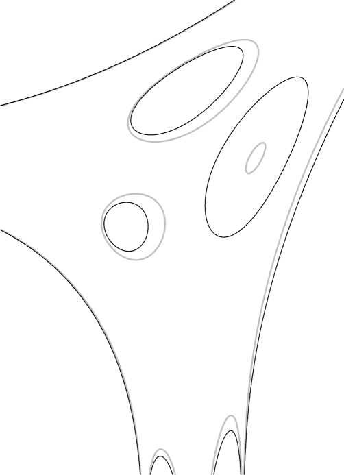
Figure 5: One oval is shrinking, the others expanding.

4.4 Volume under the Ronkin function

The maximum principle for the linearized Monge-Ampère equation used in the proof of Proposition 8 has another application for the volume under the Ronkin function.

Let $C_{1}$ and $C_{2}$ be two Harnack curves with the same boundary data and assume that their equations $P_{1}$ and $P_{2}$ are normalized in the same way (such as e.g. both constant terms are equal to 1). Then the corresponding Ronkin functions $R_{1}$ and $R_{2}$ agree asymptotically at infinity and the integral

$$\operatorname{Vol}R_{1}-\operatorname{Vol}R_{2}=\iint_{\mathbb{R}^{2}}(R_{1}-R_{2})\,dxdy$$

converges. Choosing any $R_{2}$ as our reference point, this defines a functional $\operatorname{Vol}R$ of a Harnack curve. This function has the following monotonicity in the intercept coordinates.

Proposition 9.

A variation of the curve $C$ which lowers the intercepts also lowers $\operatorname{Vol}C$. The genus zero Harnack curve is the unique volume minimizer with given boundary conditions.

Proof.

This follows from the same maximum principle used in the proof of Proposition 8: a variation which lowers the intercepts necessarily lowers the entire amoeba. The intercepts can be lowered to the unique (by Theorem 4) point where the amoeba holes shrink to points, that is, to the genus-zero curve. ∎

Theorem 5.

The variety of spectral data in (3.7) is diffeomorphic to $\mathbb{R}^{d^{2}+1}$.

Proof.

The gradient flow of the volume functional with respect to any metric on the projective space of degree $d$ curves contracts the variety of Harnack curve with given boundary to a small neighborhood of the genus zero curve. It follows that this space, together with its stratification by the genus is diffeomorphic to the product of $\binom{d-1}{2}$ copies of $\mathbb{R}_{\geq 0}$. Adding a standard divisor makes it diffeomorphic to $\mathbb{R}^{(d-1)(d-2)}$ (each hole, possibly degenerate, with a point on its boundary is diffeomorphic to an $\mathbb{R}^{2}$). Adding in the boundary points, which we showed in section 4.1 was a space diffeomorphic to $\mathbb{R}^{3d-1}$, makes $\mathbb{R}^{d^{2}+1}$. ∎

4.5 Areas of holes

Under the variation considered in Proposition 8 the area of one of the holes in the amoeba is decreasing, while the area of all other ones is increasing. Since the outer components of the amoeba complement are also expanding and the total area of the amoeba is preserved, we conclude that the decrease in the area of one hole dominates the total increase in the areas of all other holes. In other words, the Jacobian of the transformation from intercepts to the areas of holes in the amoeba is strictly diagonally dominant and, hence, nonsingular. We obtain the following

Proposition 10.

The areas on the amoeba holes can be takes as local coordinates on the manifold of Harnack curves with given boundary and genus.

This can be sharpened as follows:

Theorem 6.

The areas of the amoeba holes map the set of all Harnack curves with given boundary diffeomorphically onto $\mathbb{R}_{\geq 0}^{(d-1)(d-2)/2}$, mapping the stratification by the genus to the stratification by the number of nonzero coordinates.

Proof.

It remains to show that the map from the curve $C$ with fixed boundary to the areas of its amoeba holes is proper. Suppose that some coefficients of the equation $P(z,w)=\sum_{i,j}p_{ij}\,z^{i}w^{j}$ of $C$ grow to infinity. Recall that fixing boundary means fixing the coefficients on the boundary $\partial\Delta$ of the Newton polygon $\Delta$, so only the interior coefficients $p_{ij}$ can grow.

For each point $(i,j)$ in the interior of $\Delta$ define the convex set

$$C_{i,j}=\{(a,b)\in\mathbb{R}^{2}~{}|~{}ai+bj+\log p_{ij}\geq\max_{(k,l)\neq(i,j)}\big{(}ak+bl+\log p_{kl}\big{)}\}.$$

The union over $(i,j)$ of the $C_{i,j}$ is the set

$$\{(a,b)\in\mathbb{R}^{2}~{}|~{}\max_{(i,j)\in\Delta}\big{(}ai+bj+\log p_{ij}\big{)}\geq\max_{(i,j)\in\partial\Delta}\big{(}ai+bj+\log p_{ij}\big{)}\}.$$ (4.12)

By our assumption, this set grows to infinity, in the sense that it eventually contains a ball of any arbitrarily large radius. Therefore one of the sets $C_{i,j}$ eventually contains a ball of radius $r$, where $r$ can be arbitrarily large.

Since the Euclidean distance between $(i,j)$ and any lattice point $(k,l)\neq(i,j)$ is at least $1$, for any $(k,l)\neq(i,j)$ there exists $(a_{0},b_{0})$ satisfying $a_{0}^{2}+b_{0}^{2}\leq(r/2)^{2}$ such that

$$a_{0}(k-i)+b_{0}(l-j)\geq r/2.$$

It follows that if $C_{i,j}$ contains a ball of radius $r$, the set of $(a,b)$ satisfying

$$ai+bj+\log p_{ij}>r/2+\max_{(k,l)\neq(i,j)}\big{(}ak+bl+\log p_{kl}\big{)}\,,$$ (4.13)

contains a ball of radius $r/2$. The inequality (4.13) implies that

$$|p_{ij}\,z^{i}w^{j}|>e^{r/2}\max_{(k,l)\neq(i,j)}|p_{kl}\,z^{k}w^{l}|\,,\quad|z|=e^{a}\,,|w|=e^{b}\,,$$

therefore, all points $(a,b)$ satisfying (4.13) lie in the $(i,j)$ component of the amoeba complement provided $r$ is large enough. It follows that the area of that component is unbounded, which concludes the proof. ∎

Corollary 11.

The areas of the amoeba holes and the distances between the amoeba tentacles provide global coordinates on the moduli space of Harnack curves.

Note that the distances between the amoeba tentacles can be viewed as “renormalized” areas of the semibounded components of the amoeba complement.

5 Isoradial dimers and genus zero curves

Since Harnack curves of genus zero played a special role in our analysis, it is natural to ask for a characterization of those dimer weights that lead to spectral curves of genus zero. Genus zero weights are distinguished, for example, by maximizing the partition function for given boundary conditions.

In this section, we show that, up to gauge equivalence, genus zero weights are the same as isoradial weights studied in [14]. The results of [14] yield an explicit rational parametrization (5.2) of the spectral curve for isoradial dimers. In genus zero, the spectral curve determines the weights uniquely, up to gauge transformation. It remains, therefore, to characterize the curves (5.2) inside all genus zero Harnack curves, which is the content of Proposition 12

5.1 Isoradial embeddings

If $\Gamma$ is embedded so that every face is inscribed in a circle of radius $1$, we say that it is isoradial on condition that the weight of an edge is $\sqrt{4-\ell^{2}}$, where $\ell$ is its length. Thus the weight is the distance between the circumcenters of the two faces adjacent to the edge. See Figure 6.

Figure 6: Isoradial embedding of the honeycomb graph.

For the hexagonal lattice, an isoradial embedding with $d\times d$ fundamental domain is determined by three $d$-tuples of unit modulus complex numbers, $\{a_{1},\dots,a_{d}\},\{b_{1},\dots,b_{d}\}$ and $\{c_{1},\dots,c_{d}\}$, which are edges of the rhombi connecting vertices to the face centers as indicated in Figure 6. They obey the condition that they lie in three disjoint subintervals of the circle, that is, going counterclockwise around the circle one encounters first the $a$’s then the $b$’s then the $c$’s. It is natural to consider these parameters up to a simultaneous rotation.

5.2 Bloch-Floquet eigenfunctions

In [14] it was shown that Bloch-Floquet eigenfunctions on isoradial graphs satisfy the “local multiplier condition”, which says that if $\mathsf{b}$ and $\mathsf{w}$ are (respectively black and white) adjacent vertices on an edge bounding faces with circumcenters $C_{1}$ and $C_{2}$, then

$$f(\mathsf{b})=\frac{f(\mathsf{w})\sqrt{r_{1}r_{2}}}{(u-r_{1})(u-r_{2})}$$

where $u$ is a complex parameter and $r_{i}=C_{i}-\mathsf{w}$ are unit complex numbers. The constant $\sqrt{r_{1}r_{2}}$ does not appear in [14] due to the fact that we are using a different gauge for the Kasteleyn matrix.

In particular the eigenfunction has Floquet multipliers

$$z(u) = \frac{f(\mathsf{w}+(1,0))}{f(\mathsf{w})}=\prod_{i=1}^{d}\frac{u-a_{i}}{u-b_{i}}\sqrt{\frac{b_{i}}{a_{i}}}$$ (5.1)

$$w(u) = \frac{f(\mathsf{w}+(0,1))}{f(\mathsf{w})}=\prod_{i=1}^{d}\frac{u-c_{i}}{u-b_{i}}\sqrt{\frac{b_{i}}{c_{i}}}.$$

The parameter $u\in\mathbb{P}^{1}$ parametrizes the spectral curve $P(z,w)=0$ which is, therefore, rational. Setting

$$u=e^{it}\,,\quad a_{i}=e^{i\alpha_{i}}\,,\quad b_{i}=e^{i\beta_{i}}\,,\quad c_{i}=e^{i\gamma_{i}}\,,$$

the parametrization (5.1) becomes the following

$$z(t)=\prod_{i}\frac{\sin\frac{t-\alpha_{i}}{2}}{\sin\frac{t-\beta_{i}}{2}}\,,\quad w(t)=\prod_{i}\frac{\sin\frac{t-\gamma_{i}}{2}}{\sin\frac{t-\beta_{i}}{2}}\,,$$ (5.2)

in particular, $t\in\mathbb{R}$ parametrizes the unique nontrivial oval.

5.3 Characterization of isoradial curves

Compare (5.2) to (4.1) and note the absence of arbitrary constant factors in front. We will call curves of the form (5.2) the isoradial curves. They have the following simple characterization

Proposition 12.

A genus zero Harnack curve $C$ is isoradial if and only if the origin is in the amoeba of $C$.

Proof.

Putting $u=0$ in (5.1) we obtain a point on the unit torus, so the origin is in the amoeba of any such curve.

Conversely, making the standard change of variable from the upper half plane to unit disk in Proposition 4, we see that any Harnack curve of genus zero will have a parametrization of almost the same form as (5.1), except we have to allow two arbitrary real factors in front. Such parametrization is unique up to the $SL_{2}(\mathbb{R})$–action by automorphism of the unit disk, so we need to check whether the $SL_{2}(\mathbb{R})$–action can be used to set these arbitrary factors to $1$. Conversely, we can act by $SL_{2}(\mathbb{R})$ on (5.1) and see what kind of constant factors we can get.

Since rotating the unit disk around the origin clearly does not change anything, we have to look at the transformation

$$T(u)=\frac{u-\zeta}{1-\bar{\zeta}u}\,,\quad|\zeta|<1\,.$$

Applying it to (5.1), we obtain the parametrization:

$$\tilde{z}(u) =\prod_{i=1}^{d}\frac{|\zeta+a_{i}|}{|\zeta+b_{i}|}\,\prod_{i=1}^{d}\frac{u-\tilde{a}_{i}}{u-\tilde{b}_{i}}\sqrt{\frac{\tilde{b}_{i}}{\tilde{a}_{i}}}$$

$$\tilde{w}(u) =\prod_{i=1}^{d}\frac{|\zeta+c_{i}|}{|\zeta+b_{i}|}\,\prod_{i=1}^{d}\frac{u-\tilde{c}_{i}}{u-\tilde{b}_{i}}\sqrt{\frac{\tilde{b}_{i}}{\tilde{c}_{i}}}\,,$$

where $\tilde{a}_{i}=T^{-1}(a_{i})$ and similarly for $\tilde{b}_{i}$ and $\tilde{c}_{i}$. Comparing this with (5.1), we observe that

$$\prod_{i=1}^{d}\frac{|\zeta+a_{i}|}{|\zeta+b_{i}|}=|z(-\zeta)|\,,\quad\prod_{i=1}^{d}\frac{|\zeta+c_{i}|}{|\zeta+b_{i}|}=|w(-\zeta)|\,,$$

and hence, by its very definition, the amoeba of the curve $C$ describes the possible values of these factors. ∎

Note from the proof that the $2$-to-$1$ property implies that point $\zeta$, when it exists, is uniquely defined.

By a simple rescaling of $z$ and $w$ we can shift the amoeba of any curve $C$ so that it contains the zero. In particular, for any genus-$0$ Harnack curve this gives a canonical family of isoradial parameterizations indexed by the points in the amoeba.

References

- [1] E. Arbarello, M. Cornalba, P. Griffiths, J. Harris, Geometry of algebraic curves, Vol. I. Grundlehren der Mathematischen Wissenschaften 267. Springer-Verlag, New York, 1985.
- [2] O. Babelon, D. Bernard, M. Talon, Introduction to classical integrable systems, Cambridge University Press, 2003.
- [3] A. Beauville, Systèmes hamiltoniens complètement intégrables associés aux surfaces , Problems in the theory of surfaces and their classification (Cortona, 1988), 25–31, Sympos. Math., XXXII, Academic Press, London, 1991.
- [4] A. Beauville, Determinantal hypersurfaces, Michigan Math. J. 48 (2000), 39–64.
- [5] R. J. Cook and A. D. Thomas, Line bundles and homogeneous matrices, Quart. J. Math. Oxford (2), 30 (1979), 423–429.
- [6] Dynamical systems, VII, edited by V. I. Arnold and S. P. Novikov, Encyclopaedia of Mathematical Sciences, Vol. 16, Springer-Verlag, Berlin, 1994.
- [7] I. Dynnikov and S. Novikov, Discrete spectral symmetries of small-dimensional differential operators and difference operators on regular lattices and two-dimensional manifolds, Russian Math. Surveys 52 (1997), no. 5, 1057–1116.
- [8] I. Dynnikov and S. Novikov, Geometry of the triangle equation on two-manifolds, math-ph/0208041.
- [9] D. Gieseker, H. Knörrer, E. Trubowitz, The geometry of algebraic Fermi curves, Perspectives in Mathematics, Vol. 14, Academic Press, 1993.
- [10] A. Gorsky, N. Nekrasov, V. Rubtsov, Hilbert schemes, separated variables, and D-branes, Comm. Math. Phys. 222 (2001), no. 2, 299–318.
- [11] J. Hurtubise, Integrable systems and algebraic surfaces, Duke Math. J. 83 (1996), no. 1, 19–50.
- [12] P. Kasteleyn, Statistics of dimers on a lattice, …
- [13] R. Kenyon, An introduction to the dimer model, math.CO/0310326.
- [14] R. Kenyon, The Laplacian and operators on critical planar graphs Invent. Math. 150 (2002), 409-439.
- [15] R. Kenyon, A. Okounkov, S. Sheffield Dimers and amoebae, to appear.
- [16] G. Mikhalkin, Real algebraic curves, the moment map and amoebas, Ann. of Math. (2) 151 (2000), no. 1, 309–326.
- [17] G. Mikhalkin and H. Rullgård, Amoebas of maximal area, Internat. Math. Res. Notices 2001, no. 9, 441–451.
- [18] A. Oblomkov, Difference operators on two-dimensional regular lattices, Theoret. and Math. Phys. 127 (2001), no. 1, 435–445.
- [19] J. Propp, Generalized domino shuffling, math.CO/0111034.
- [20] E. Sklyanin, Separation of variables—new trends, Quantum field theory, integrable models and beyond (Kyoto, 1994). Progr. Theoret. Phys. Suppl. No. 118, (1995), 35–60.
- [21] V. Vinnikov, Selfadjoint determinantal representations of real plane curves, Math. Ann. 296 (1993), no. 3, 453–479.