The Compactification of the Moduli Space of Convex $\mathbb{RP}^{2}$ Surfaces, I

1. Introduction

In [16] Goldman proves that the deformation space $\mathcal{G}_{g}$ of convex $\mathbb{RP}^{2}$ structures on an oriented closed surface of genus $g\geq 2$ is a cell of $16g-16$ real dimensions. He constructs explicit coordinates of the space based on a Fenchel-Nielsen type pants decomposition of the surface. In particular, for each boundary geodesic loop in this decomposition, there is a holonomy map in $\mathbf{PGL}(3,\mathbb{R})$, unique up to conjugacy, which measures how a choice of $\mathbb{RP}^{2}$ coordinates develops around the loop.

In [24, 26] there is another proof of Goldman’s theorem which introduces new coordinates on $\mathcal{G}$. Using a developing map due to C.P. Wang [29] and deep results in affine differential geometry of Cheng-Yau [4, 5], there is a natural correspondence between a convex $\mathbb{RP}^{2}$ structure on a surface of genus $g\geq 2$ and a pair $(\Sigma,U)$ of a conformal structure $\Sigma$ and a holomorphic cubic differential $U$ on $\Sigma$. This shows that $\mathcal{G}_{g}$ is the total space of a $5g-5$ complex dimensional vector bundle over Teichmüller space, and so by Riemann-Roch, $\mathcal{G}_{g}$ is a cell of complex dimension $8g-8$.

Wang’s formulation does give a way to calculate the holonomy by a first-order linear system of PDEs, but unfortunately the data depends on the solution to a separate nonlinear PDE (31) below, and thus it seems we cannot hope to use this to relate the two coordinate systems. However, on a noncompact Riemann surface of finite type, we can force solutions of (31) to behave well near the punctures, and in fact calculate the holonomy around a loop at each puncture.

Theorem 1.

Given a Riemann surface $\Sigma$ of finite type, and a holomorphic cubic differential $U$ on $\Sigma$ with poles of order 3 allowed at each puncture. Let $R_{i}$ be the residue at each puncture. Then there is an $\mathbb{RP}^{2}$ structure corresponding to $(\Sigma,U)$. The $\mathbb{RP}^{2}$ holonomy type around each puncture is determined by the $R_{i}$.

A more explicit version of this theorem is given below as Theorem 5. The space of all residues $R\in\mathbb{C}$ maps two-to-one onto the space of holonomy types if ${\rm Re}\,R\neq 0$. These two cases are distinguished by another of Goldman’s coordinates, the vertical twist parameter, which in part corresponds to the twist parameter in Fenchel-Nielsen theory. The vertical twist parameter approaching $\infty$ roughly corresponds stretching the $\mathbb{RP}^{2}$ structure along a neck.

Theorem 2.

Given a pair $(\Sigma,U)$ as above, at a puncture with residue $R_{i}$ with ${\rm Re}\,R_{i}\neq 0$, the vertical twist parameter of the $\mathbb{RP}^{2}$ structure at that puncture is $\pm\infty$, the sign being equal to the sign of ${\rm Re}\,R_{i}$.

This theorem combines Propositions 12 and 14 below.

There are natural examples of such pairs $(\Sigma,U)$ at the boundary of the total space of the space of cubic differentials over the moduli space of Riemann surfaces $\overline{\mathcal{M}}_{g}$. In particular, at a nodal curve at the boundary of $\mathcal{M}_{g}$, regular cubic differentials have poles of order at most 3 at the nodes, with opposite residues across each side of the node.

Theorem 3.

On the total space of the (V-manifold) vector bundle of regular cubic differentials over $\overline{\mathcal{M}}_{g}$, the holonomy type and vertical twist parameters vary continuously.

This theorem is made more precise below in Theorem 6. In particular, we must also make a mild technical assumption on families of cubic differentials which approach regular cubic differentials with residue 0.

The proof of these results relies on a fundamental correspondence due to Cheng-Yau [4, 5], that each convex bounded domain $\Omega\subset\mathbb{RP}^{n}$ may be canonically identified with a hypersurface, the hyperbolic affine sphere $H\subset\mathbb{R}^{n+1}$ which is asymptotic to the boundary of the cone $\mathcal{C}(\Omega)$ over $\Omega$. Any projective group $\Gamma\subset\mathbf{PGL}(n+1,\mathbb{R})$ which acts on $\Omega$ lifts to a linear group which acts on $\mathbb{R}^{n+1}$ and takes $H$ to itself, and natural differential geometric structure descends to any manifold $\Omega/\Gamma\equiv H/\Gamma$. This theory is reviewed in Section 3 below. See also [24, 26].

In dimension $n=2$, there is a natural system of first-order PDEs which develop any hyperbolic affine sphere in $\mathbb{R}^{3}$ [29, Wang]. (Wang’s theory is analogous to the more familiar case of minimal surfaces in $\mathbb{R}^{3}$.) We give a version of this formulation in Section 4 below. In particular, given a Riemann surface $\Sigma$ with conformal metric $h$, a cubic differential $U$ over $\Sigma$, and a function $u$ so that

(1) $$\Delta u=-4e^{-2u}\|U\|^{2}+2e^{u}+2\kappa,$$

there is a system of first-order PDEs (18-28) below which integrate the structure equations for a hyperbolic affine sphere to give a map from the universal cover of $\Sigma$ to a hyperbolic affine sphere $H$. Moreover, Cheng-Yau [5] guarantees that if the metric $e^{u}h$ is complete, then $H$ is asymptotic to the boundary of a convex cone $\mathcal{C}(\Omega)$ for a domain $\Omega$ as in the previous paragraph. So given $(\Sigma,U)$ and a function $u$ satisfying (1), there is a convex $\mathbb{RP}^{2}$ structure on $\Sigma$. Moreover, the first-order PDE system (18-28) naturally calculates the holonomy of the $\mathbb{RP}^{2}$ structure around any loop. This relates the affine differential geometry of Wang and Cheng-Yau to Goldman’s coordinates on the deformation space $\mathcal{G}$ of convex $\mathbb{RP}^{2}$ structures. Goldman’s coordinates on the deformation space of convex $\mathbb{RP}^{2}$ structures are discussed in Section 2 below.

Wang solved his PDE (1) to find a unique solution on any compact Riemann surface of genus $g\geq 2$. In Section 5 below, we extend this to a complete hyperbolic Riemann surface $\Sigma$ of finite type with cubic differential $U$ which has poles of order 3 at each puncture. We find an Ansatz metric $h$ on $\Sigma$ in order to find a solution $u$ to (1) which behaves well near each puncture. In particular, we construct a barrier to bound $u$ near each puncture. Then calculating the holonomy around each puncture involves solving a linear systems of ODEs which is asymptotic to a constant coefficient system as we approach the puncture. This allows us to determine the eigenvalues of the holonomy matrix in terms of the residue $R$ of $U$ ($R$ is the leading coefficient of the Laurent series of $U$ at the puncture). The actual conjugacy type is more subtle if the eigenvalues are repeated. In particular, a geometric result of Choi [7] rules out certain holonomy types. See Section 6 below.

In Section 7 we use Wang’s developing map (18-28) to provide more information about the structure of the $\mathbb{RP}^{2}$ structure near the punctures. In particular (if the residue $R\neq 0$), along certain paths which approach the puncture, the (18-28) restrict to a system of ODEs of the form

$$\partial_{y}\mathbf{X}=[\mathbf{B}+\mathbf{E}(x,y)]\mathbf{X},$$

where $\mathbf{B}$ is a constant matrix and the error term $\mathbf{E}(x,y)$ decays exponentially as $y\to\infty$. These equations have been extensively studied, originally by Dunkel [12]. In Appendix A, we extend estimates on solutions of such systems to the case of a parameter $x$. In particular, we can determine that the vertical twist parameter at each such end is $\pm\infty$, the sign agreeing with that of ${\rm Re}\,R$.

Finally, in Section 8, we extend these results to families of pairs $(\Sigma_{t},U_{t})$ in which $\Sigma_{t}$ tends to a nodal curve at the boundary of the Deligne-Mumford compactification $\overline{\mathcal{M}}_{g}$ of the moduli space of Riemann surfaces, and the cubic differential $U_{t}$ over $\Sigma_{t}$ tends to a regular cubic differential over the nodal curve. A regular cubic differential allows poles of order 3 at either side of the node, and the residues $R,R^{\prime}$ at either side of the node satisfy $R=-R^{\prime}$. We first review the analytic theory of $\overline{\mathcal{M}}_{g}$ in terms of plumbing coordinates which replace each node by a thin neck. Our barriers extend across the neck to control a solution $u_{t}$ to (1). Thereby, the holonomy and vertical twist parameters along this end behave well in families. (Controlling the vertical twist parameters in families involves some fairly subtle analysis to fix a natural gauge. Here the extension of Dunkel’s theorem to systems with parameters in Appendix A is essential.)

As mentioned above, Goldman worked out the analog of Fenchel-Nielsen coordinates on $\mathcal{G}_{g}$ [16]. In general, one would like to extend the rich theory of Teichmüller space to $\mathcal{G}_{g}$. The symplectic theory is worked out rather well: There is a natural symplectic form on $\mathcal{G}_{g}$ due to Goldman [15, 17] which extends the Weil-Petersson symplectic form on Teichmüller space. Kim [23] has used Goldman’s coordinates to show that $\mathcal{G}_{g}$ is naturally symplectomorphic to $\mathbb{R}^{16g-16}$, which extends a result of Wolpert [33] about Teichmüller space.

Another example of this is provided by Hitchin [22], who finds a connected component, the Teichmüller component, of the space of representations of $\pi_{1}(\Sigma_{g})$ into $\mathbf{PGL}(n,\mathbb{R})$ for all $n$. In the case $n=3$, the Teichmüller component is given by the space $H^{0}(\Sigma,K^{2})\oplus H^{0}(\Sigma,K^{3})$ for a fixed complex structure on $\Sigma$. This space may be identified by $\mathcal{G}_{g}$ by the holonomy representation of the $\mathbb{RP}^{2}$ structure [9, Choi-Goldman]. In particular, Hitchin extends the theory of Higgs bundles he earlier used to study Teichmüller space itself in [21] to study representation spaces into Lie groups. We should remark that François Labourie has shown in unpublished work that if the $H^{0}(\Sigma,K^{2})$ part of Hitchin’s correspondence is zero, then Hitchin’s cubic differential may be identified Wang’s cubic differential.

We should also mention that Darvishzadeh-Goldman [11] have constructed an analog of the Weil-Petersson metric on $\mathcal{G}_{g}$ which interacts with the symplectic form to form an almost complex, and indeed, and almost Kähler structure. It is not clear if this almost complex structure is integrable or how it might relate to the complex structure provided by the pairs $(\Sigma,U)$.

On the compactified moduli space of Riemann surfaces $\overline{\mathcal{M}}_{g}$, there has been extensive work relating the complex structure of $\overline{\mathcal{M}}_{g}$ as a V-manifold with the geometry provided by the hyperbolic metric (i.e. the Fenchel-Nielsen coordinates). See in particular Wolf [30] and Wolpert [34]. The present work is an attempt to extend this theory to the moduli space of $\mathbb{RP}^{2}$ structures. In particular, the space of pairs $(\Sigma,U)$ of a Riemann surface $\Sigma$ of genus $g\geq 2$ and a cubic differential $U$ over $\Sigma$ is naturally partially compactified to be the total space of a (V-manifold) vector bundle $\mathcal{S}\to\overline{\mathcal{M}}_{g}$, where the fiber of $\mathcal{S}$ is the space of regular cubic differentials over the possibly singular curve $\Sigma$. This provides a natural complex structure on a partial compactification of the moduli space of convex $\mathbb{RP}^{2}$ structures on oriented surfaces of genus $g$. The $\mathbb{RP}^{2}$ structure on $\Sigma$ is the analog of the hyperbolic metric, and we relate this complex structure on $\mathcal{S}$ to the coordinates on $\mathcal{G}_{g}$ given by Goldman. In this work we only address the holonomy and twist parameters around a neck which is being pinched to a node. We hope to address the other coordinates in Goldman’s chart in future work. Also, we only address the topological relationship between $\mathcal{S}$ and Goldman’s coordinates in this paper. Eventually one might be able to study relationship between the two coordinates real-analytically. This point is already complicated in the case of $\overline{\mathcal{M}}_{g}$ [31, Wolf-Wolpert].

There are nonconvex $\mathbb{RP}^{2}$ structures on surfaces, which are classified by Choi [6, 7, 8].

Also, there is recent work of Benoist on compactifying the space of faithful representations of a finite-type group $\rho:\Gamma\to\mathbf{PGL}(n+1,\mathbb{R})$ so that there is a properly convex $\Gamma$-invariant domain $\Omega\subset\mathbb{RP}^{n}$ so that $\Omega/\rho(\Gamma)$ is compact [benoist03]. This extends the theorem of Choi-Goldman [9] to higher dimensions.

Acknowledgements.

I would like to thank S.-T. Yau, Curt McMullen, Bill Goldman, Suhyoung Choi, and Scott Wolpert, Michael Thaddeus, Ravi Vakil, Richard Wentworth for useful conversations. I would like to thank Curt McMullen especially for suggesting that there should be a relationship between the residues of the cubic differentials and the $\mathbb{RP}^{2}$ holonomy of the end.

2. Goldman’s coordinates

An $\mathbb{RP}^{n}$ structure on a manifold $M$ consists of a maximal atlas of charts in $\mathbb{RP}^{n}$ with transition maps in $\mathbf{PGL}(n+1,\mathbb{R})$. We may also call $M$ an $\mathbb{RP}^{n}$ manifold. Note that the straight lines in any coordinate chart in $\mathbb{RP}^{n}$ are preserved by the transition maps. A path in $M$ which in any such coordinate chart is a straight line is called an $\mathbb{RP}^{n}$ geodesic. Also, given an $\mathbb{RP}^{n}$ manifold $M$ and a coordinate chart in $\mathbb{RP}^{n}$ around a point $p$, analytic continuation induces a map, the developing map dev extending the coordinate chart map from the universal cover $\tilde{M}$ of $M$ (with basepoint $p$) to $\mathbb{RP}^{n}$. Also, there is a holonomy homomorphism hol from $\pi_{1}M$ to $\mathbf{PGL}(n+1,\mathbb{R})$ so that $\forall\gamma\in\pi_{1}M$,

$${\rm dev}\circ\gamma={\rm hol}(\gamma)\circ{\rm dev}.$$

For any other choice of basepoint and/or coordinate chart, there is a map $g\in\mathbf{PGL}(n+1,\mathbb{R})$ so that

$${\rm dev}^{\prime}=g\circ{\rm dev}\quad\mbox{and}\quad{\rm hol}^{\prime}(\gamma)=g\circ{\rm hol}(\gamma)\circ g^{-1}.$$

For more details, see e.g. Goldman [16]. In particular, the holonomy map is unique up to conjugation in $\mathbf{PGL}(n+1,\mathbb{R})$.

$M$ is a convex $\mathbb{RP}^{n}$ manifold if dev$:\tilde{M}\mapsto\mathbb{RP}^{n}$ is a diffeomorphism onto a domain $\Omega$ so that $\Omega$ is a convex subset of some $\mathbb{R}^{n}\subset\mathbb{RP}^{n}$. $M$ is called properly convex if in addition $\Omega$ is properly contained in some $\mathbb{R}^{n}\subset\mathbb{RP}^{n}$. In this case, there is a representation hol of $\Gamma=\pi_{1}M$ into $\mathbf{PGL}(n+1,\mathbb{R})$ so that $\Gamma$ acts discretely and properly discontinuously on $\Omega$. The quotient $\Omega/\Gamma$ is our $\mathbb{RP}^{n}$ manifold $M$. See e.g. [16] for details.

In [16], Goldman introduced coordinates on the deformation space of convex real projective structures on a given closed oriented surface $S$ of genus $g\geq 2$. These coordinates are analogous to Fenchel-Nielsen coordinates on Teichmüller space. We may cut $S$ into $2g-2$ pairs of pants so that the boundary of each pair of pants is an $\mathbb{RP}^{2}$ geodesic, i.e. is a straight line in an projective coordinate chart. Around each of these geodesic loops is a holonomy action, which may be represented as a matrix $H$ in $\mathbf{SL}(3,\mathbb{R})$ once we choose an appropriate frame. The conjugacy class of this matrix is invariant of our choice and constitutes the analog of Fenchel-Nielsen’s length parameter. The eigenvalues of the holonomy matrix $H$ are real, positive, and distinct. So the holonomy type may be described by the set of eigenvalues

$$\{\alpha_{1},\alpha_{2},\alpha_{3}\},\quad\alpha_{i}\in\mathbb{R}^{+},\quad\alpha_{1}\alpha_{2}\alpha_{3}=1,\quad\alpha_{i}\neq\alpha_{j}\mbox{ for }i\neq j.$$

Matrices in $\mathbf{SL}(3,\mathbb{R})$ whose eigenvalues satisfy these conditions are called hyperbolic. Order the eigenvalues $\alpha_{i}$ so that the standard form of a hyperbolic holonomy matrix is

(2) $$\mathbf{D}(\alpha_{1},\alpha_{2},\alpha_{3})\quad\alpha_{1}>\alpha_{2}>\alpha_{3}>0$$

(Here $\mathbf{D}$ denotes the diagonal matrix.)

There are three fix points of this hyperbolic holonomy matrix: Fix${}^{+}=[1,0,0]$ is attracting, Fix${}^{-}=[0,0,1]$ is repelling, and Fix${}^{0}=[0,1,0]$ is a saddle fixed point. The holonomy acts on each coordinate line in $\mathbb{RP}^{2}$, and these lines split $\mathbb{RP}^{2}$ into four triangles. Fix one open triangle $T$ to be the projection of the first octant in $\mathbb{R}^{3}$ to $\mathbb{RP}^{2}$. The boundary of $T$ is formed by three line segments: $G^{+0}$ connects Fix⁺ to Fix⁰, $G^{0-}$ connects Fix⁰ to Fix^-, and $G^{+-}$ connected Fix⁺ to Fix^-. $G^{+-}$ is called the principal geodesic segment for the holonomy action. See Figure 1.

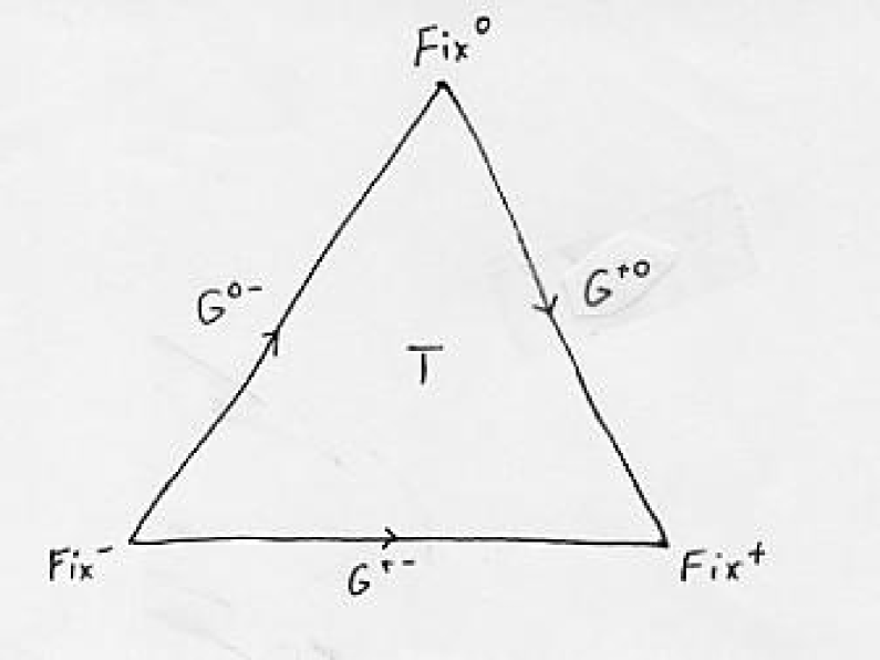
Figure 1. The Principal Triangle

We will also need to consider two other types of holonomy which are degenerate in that they cannot occur in closed $\mathbb{RP}^{2}$ surfaces. The first is quasi-hyperbolic holonomy, in which the holonomy matrix is conjugate to

$$\left(\begin{array}[]{ccc}\alpha_{1}&1&0\\ 0&\alpha_{1}&0\\ 0&0&\alpha_{3}\end{array}\right)\quad\mbox{for}\quad\alpha_{i}>0,\quad\alpha_{1}^{2}\alpha_{3}=1,\quad\alpha_{1}\neq\alpha_{3}.$$

Also we will consider parabolic holonomy, in which the holonomy matrix is conjugate to

$$\left(\begin{array}[]{ccc}1&1&0\\ 0&1&1\\ 0&0&1\end{array}\right).$$

Choi [7] discusses all the types of holonomy which can appear in an oriented $\mathbb{RP}^{2}$ surface. We describe the dynamics of quasi-hyperbolic and parabolic holonomies is Subsections 7.5 and 7.6 respectively.

There are also twist parameters analogous to those in Fenchel-Nielsen theory. We recall the discussion in Goldman [16]. Around any oriented simple homotopically nontrivial loop in a compact, convex $\mathbb{RP}^{2}$ surface $S=S_{0}$, the holonomy type is hyperbolic. Inside the homotopy class of such a loop, there is a unique representative which is a simple closed principal geodesic loop $\mathcal{L}$. Then we may cut the surface $S_{0}$ along $\mathcal{L}$ to form a possibly disconnected $\mathbb{RP}^{2}$ surface $S_{0}^{\rm cut}$ with principal geodesic boundary. For simplicity, we discuss only the case where $S_{0}^{\rm cut}=S^{a}_{0}\sqcup S^{b}_{0}$ is disconnected. The other case is similar. Choose $\mathbb{RP}^{2}$ coordinates on $S_{0}^{a}$ near the principal boundary geodesic so that the holonomy matrix $H$ is in the standard form (2), the principal boundary geodesic $\mathcal{L}$ develops to the standard $G^{+-}$, and the developed image of $S_{0}^{a}$ does not intersect the interior of $T$. Then the other component $S_{0}^{b}$ is attached along $G^{+-}$ by placing the image of its developing map inside $T$ across $G^{+-}$ from ${\rm dev}\widetilde{S_{0}^{a}}$. (The inverse image of $\mathcal{L}$ in the universal cover $\Omega=\widetilde{S_{0}}$ consists of not just the line segment $G^{+-}$, but also a line segment $\rm{hol}(\beta)G^{+-}$ for each $\beta$ in the coset space $\pi_{1}S_{0}/\langle\gamma\rangle$, where $\gamma$ is the element in $\pi_{1}S_{0}$ determined by $\mathcal{L}$. We must do a similar gluing across each of these line segments. For simplicity, we focus on just the gluing across $G^{+-}$.)

The $\mathbb{RP}^{2}$ structure on the glued surface $S_{0}=S^{a}_{0}\cup_{\mathcal{L}}S^{b}_{0}$ is then determined by an orientation-reversing projective diffeomorphism $J$ from a neighborhood $N^{a}\subset S^{a}_{0}$ of $\mathcal{L}$ to a similar neighborhood $N^{b}\subset S^{b}_{0}$. In terms of coordinates in the developed image near $G^{+-}$, $J$ may be represented as the diagonal matrix $\mathbf{D}(1,-1,1)$, which commutes with the holonomy matrix $H$.

Now the twist parameters come in. For real $(\sigma,\tau)$ consider the twist matrix

$$\mathbf{M}(\sigma,\tau)=\mathbf{D}(e^{-\sigma-\tau},e^{2\tau},e^{\sigma-\tau}).$$

Then we form a new $\mathbb{RP}^{2}$ surface $S_{\sigma,\tau}$ by gluing the neighborhood $S^{b}_{0}$ by the projective involution $J_{\sigma,\tau}=\mathbf{M}(\sigma,\tau)J$ instead of the standard $J$. See Figure 2. Let dev_σ,τ be equal to the standard developing map on $\widetilde{S^{a}_{0}}$ as in the previous paragraph, and extend to all of $\widetilde{S_{\sigma,\tau}}$ by using the gluing map $J_{\sigma,\tau}$. We adapt Kim’s terminology in [23] to call $\sigma$ the horizontal twist parameter and $\tau$ the vertical twist parameter. For the $\mathbb{RP}^{2}$ structure determined by a hyperbolic Riemann surface, $\sigma$ corresponds to the usual Fenchel-Nielsen twist parameter.

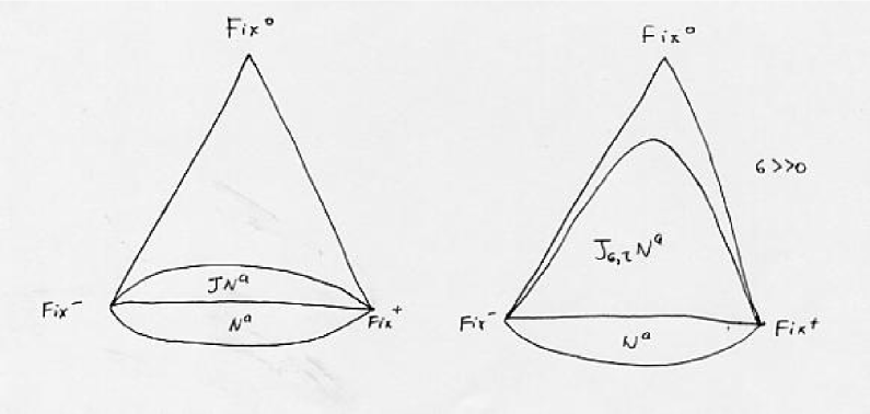
Figure 2. Twist Parameters

Note that as the vertical twist parameter $\tau\to+\infty$, the image of the developing map dev${}_{\sigma,\tau}(\widetilde{S_{\sigma,\tau}})$ expands to include all the interior of the principal triangle $T$. In this case we have attached the entire principal half-annulus $\mathcal{A}=T/\langle H\rangle$ to $S^{a}_{0}$ along the principal boundary geodesic $\mathcal{L}$. There is only one way to attach this principal half-annulus as an $\mathbb{RP}^{2}$ surface without boundary. (Although there are two distinct ways to put a non-principal geodesic boundary on $S^{a}_{0}\cup_{\mathcal{L}}\mathcal{A}$—see e.g. Choi-Goldman [10].)

Similarly if $\tau\to-\infty$, dev${}_{\sigma,\tau}(\widetilde{S_{\sigma,\tau}})$ shrinks so that the glued part of dev${}_{\sigma,\tau}(\widetilde{S^{b}_{0}})$ vanishes, and dev${}_{\sigma,\tau}(\widetilde{S_{\sigma,\tau}})$ does not intersect the principal triangle $T$. In this case, the principal geodesic segment $\mathcal{L}$ is a natural boundary for the limit $\mathbb{RP}^{2}$ surface.

Goldman [16] also introduces interior parameters associated to each pair of pants. See also Kim [23]. We hope to use the methods of this paper to analyze them in future work.

3. Hyperbolic affine spheres and convex $\mathbb{RP}^{n}$ structures

Recall the standard definition of $\mathbb{RP}^{n}$ as the set of lines through 0 in $\mathbb{R}^{n+1}$. There is a map $P\!:\mathbb{R}^{n+1}\setminus 0\to\mathbb{RP}^{n}$ with fiber $\mathbb{R}^{*}$. For a convex domain $\Omega\subset\mathbb{R}^{n}\subset\mathbb{RP}^{n}$ as above, then $P^{-1}(\Omega)$ has two connected components. Call one such component $\mathcal{C}(\Omega)$, the cone over $\Omega$. Then any representation of a group $\Gamma$ into $\mathbf{PGL}(n+1,\mathbb{R})$ so that $\Gamma$ acts discretely and properly discontinously on $\Omega$ lifts to a representation into

$$\mathbf{SL}^{\pm}(n+1,\mathbb{R})=\{A\in\mathbf{GL}(n+1,\mathbb{R}):\det A=\pm 1\}$$

which acts on $\mathcal{C}(\Omega)$. See e.g. [26].

For a properly convex $\Omega$, then there is a unique hypersurface asymptotic to the boundary of the cone $\mathcal{C}(\Omega)$ called the hyperbolic affine sphere [2, 4, 5]. This hyperbolic affine sphere $H\subset\mathcal{C}$ is invariant under automorphisms of $\mathcal{C}(\Omega)$ in $\mathbf{SL}^{\pm}(n+1,\mathbb{R})$. The projection map $P$ induces a diffeomorphism of $H$ onto $\Omega$. Affine differential geometry provides $\mathbf{SL}^{\pm}(n+1,\mathbb{R})$-invariant structure on $H$ which then descends to $M=\Omega/\Gamma$. In particular, both the affine metric, which is a Riemannian metric conformal to the (Euclidean) second fundamental form of $H$, and a projectively flat connection whose geodesics are the $\mathbb{RP}^{n}$ geodesics on $M$, descend to $M$. See [26] for details. A fundamental fact about hyperbolic affine spheres is due to Cheng-Yau [5] and Calabi-Nirenberg (unpublished):

Theorem 4.

If the affine metric on a hyperbolic affine sphere $H$ is complete, then $H$ is properly embedded in $\mathbb{R}^{n+1}$ and is asymptotic to a convex cone $\mathcal{C}\subset\mathbb{R}^{n+1}$ which contains no line. By a volume-preserving affine change of coordinates in $\mathbb{R}^{n+1}$, we may assume $\mathcal{C}=\mathcal{C}(\Omega)$ for some properly convex domain $\Omega$ in $\mathbb{RP}^{n}$.

Below in Section 4, we recall a theory due to C.P. Wang in the case $n=2$ and $M$ is oriented. In this case, a properly convex $\mathbb{RP}^{2}$ structure is given by certain data on a Riemann surface $\Sigma$, and the developing map is given explicitly in terms of these data by the solution to a first-order linear system of PDEs.

4. Wang’s developing map

C.P. Wang formulates the condition for a two-dimensional surface to be an affine sphere in terms of the conformal geometry given by the affine metric [29]. Since we rely heavily on this work, we give a version of the arguments here for the reader’s convenience. For basic background on affine differential geometry, see Calabi [2], Cheng-Yau [5] and Nomizu-Sasaki [28].

Choose a local conformal coordinate $z=x+iy$ on the hypersurface. Then the affine metric is given by $h=e^{\psi}|dz|^{2}$ for some function $\psi$. Parametrize the surface by $f:\mathcal{D}\rightarrow\mathbb{R}^{3}$, with $\mathcal{D}$ a domain in $\mathbb{C}$. Since $\{e^{-\frac{1}{2}\psi}f_{x},e^{-\frac{1}{2}\psi}f_{y}\}$ is an orthonormal basis for the tangent space, the affine normal $\xi$ must satisfy this volume condition (see e.g. [28])

$$\det(e^{-\frac{1}{2}\psi}f_{x},e^{-\frac{1}{2}\psi}f_{y},\xi)=1,$$

which implies

(3) $$\det(f_{z},f_{\bar{z}},\xi)={\textstyle\frac{1}{2}}ie^{\psi}.$$

Now only consider hyperbolic affine spheres. By scaling in $\mathbb{R}^{3}$, we need only consider spheres with affine mean curvature $-1$. In this case, we have the following structure equations:

(4) $$\left\{\begin{array}[]{c}D_{X}Y=\nabla_{X}Y+h(X,Y)\xi\\ D_{X}\xi=X\end{array}\right.$$

Here $D$ is the canonical flat connection on $\mathbb{R}^{3}$, $\nabla$ is a projectively flat connection, and $h$ is the affine metric. If the center of the affine sphere is $0$, then we also have $\xi=f$.

It is convenient to work with complexified tangent vectors, and we extend $\nabla$, $h$ and $D$ by complex linearity. Consider the frame for the tangent bundle to the surface $\{e_{1}=f_{z}=f_{*}(\frac{\partial}{\partial z}),e_{\bar{1}}=f_{\bar{z}}=f_{*}(\frac{\partial}{\partial{\bar{z}}})\}$. Then we have

(5) $$h(f_{z},f_{z})=h(f_{\bar{z}},f_{\bar{z}})=0,\quad h(f_{z},f_{\bar{z}})={\textstyle\frac{1}{2}}e^{\psi}.$$

Consider $\theta$ the matrix of connection one-forms

$$\nabla e_{i}=\theta^{j}_{i}e_{j},\quad i,j\in\{1,{\bar{1}}\},$$

and ${\hat{\theta}}$ the matrix of connection one-forms for the Levi-Civita connection. By (5)

(6) $${\hat{\theta}}^{1}_{\bar{1}}={\hat{\theta}}^{\bar{1}}_{1}=0,\quad{\hat{\theta}}^{1}_{1}=\partial\psi,\quad{\hat{\theta}}^{\bar{1}}_{\bar{1}}={\bar{\partial}}\psi.$$

The difference ${\hat{\theta}}-\theta$ is given by the Pick form. We have

$${\hat{\theta}}^{j}_{i}-\theta^{j}_{i}=C^{j}_{ik}\rho^{k},$$

where $\{\rho^{1}=dz,\rho^{\bar{1}}=d{\bar{z}}\}$ is the dual frame of one-forms. Now we differentiate (3) and use the structure equations (4) to conclude

$$\theta^{1}_{1}+\theta^{\bar{1}}_{\bar{1}}=d\psi.$$

This implies, together with (6), the apolarity condition

$$C^{1}_{1k}+C^{\bar{1}}_{{\bar{1}}k}=0,\quad k\in\{1,{\bar{1}}\}.$$

Then, when we lower the indices, the expression for the metric (5) implies that

$$C_{{\bar{1}}1k}+C_{1{\bar{1}}k}=0.$$

Now $C_{ijk}$ is totally symmetric on three indices [5, 28]. Therefore, the previous equation implies that all the components of $C$ must vanish except $C_{111}$ and $C_{{\bar{1}}{\bar{1}}{\bar{1}}}=\overline{C_{111}}$.

This discussion completely determines $\theta$:

(7) $$\left(\begin{array}[]{cc}\theta^{1}_{1}&\theta^{1}_{\bar{1}}\\[2.84526pt] \theta^{\bar{1}}_{1}&\theta^{\bar{1}}_{\bar{1}}\end{array}\right)=\left(\begin{array}[]{cc}\partial\psi&C^{1}_{{\bar{1}}{\bar{1}}}d{\bar{z}}\\[2.84526pt] C^{\bar{1}}_{11}dz&\bar{\partial}\psi\end{array}\right)=\left(\begin{array}[]{cc}\partial\psi&\bar{U}e^{-\psi}d{\bar{z}}\\ Ue^{-\psi}dz&\bar{\partial}\psi\end{array}\right),$$

where we define $U=C^{\bar{1}}_{11}e^{\psi}$.

Recall that $D$ is the canonical flat connection induced from ${\mathbb{R}}^{3}$. (Thus, for example, $D_{f_{z}}f_{z}=D_{\frac{\partial}{\partial z}}f_{z}=f_{zz}$.) Using this statement, together with (5) and (7), the structure equations (4) become

(8) $$\left\{\begin{array}[]{c}f_{zz}=\psi_{z}f_{z}+Ue^{-\psi}f_{\bar{z}}\\ f_{{\bar{z}}{\bar{z}}}={\bar{U}}e^{-\psi}f_{z}+\psi_{\bar{z}}f_{\bar{z}}\\ f_{z{\bar{z}}}=\frac{1}{2}e^{\psi}f\end{array}\right.$$

Then, together with the equations $f_{z}=f_{z}$ and $f_{\bar{z}}=f_{\bar{z}}$, these form a linear first-order system of PDEs in $f$, $f_{z}$ and $f_{\bar{z}}$:

(18) $$\frac{\partial}{\partial z}\left(\begin{array}[]{c}f\\ f_{z}\\ f_{\bar{z}}\end{array}\right) = \left(\begin{array}[]{ccc}0&1&0\\ 0&\psi_{z}&Ue^{-\psi}\\ \frac{1}{2}e^{\psi}&0&0\end{array}\right)\left(\begin{array}[]{c}f\\ f_{z}\\ f_{\bar{z}}\end{array}\right),$$

(28) $$\frac{\partial}{\partial\bar{z}}\left(\begin{array}[]{c}f\\ f_{z}\\ f_{\bar{z}}\end{array}\right) = \left(\begin{array}[]{ccc}0&0&1\\ \frac{1}{2}e^{\psi}&0&0\\ 0&\bar{U}e^{-\psi}&\psi_{\bar{z}}\\ \end{array}\right)\left(\begin{array}[]{c}f\\ f_{z}\\ f_{\bar{z}}\end{array}\right).$$

In order to have a solution of the system (8), the only condition is that the mixed partials must commute (by the Frobenius theorem). Thus we require

(29) $$\psi_{z{\bar{z}}}+|U|^{2}e^{-2\psi}-{\textstyle\frac{1}{2}}e^{\psi} = 0,$$

$$U_{\bar{z}} = 0.$$

The system (8) is an initial-value problem, in that given (A) a base point $z_{0}$, (B) initial values $f(z_{0})\in\mathbb{R}^{3}$, $f_{z}(z_{0})$ and $f_{\bar{z}}(z_{0})=\overline{f_{z}(z_{0})}$, and (C) $U$ holomorphic and $\psi$ which satisfy (29), we have a unique solution $f$ of (8) as long as the domain of definition $\mathcal{D}$ is simply connected. We then have that the immersion $f$ satisfies the structure equations (4). In order for $f$ to be the affine normal of $f(\mathcal{D})$, we must also have the volume condition (3), i.e. $\det(f_{z},f_{\bar{z}},f)=\frac{1}{2}ie^{\psi}$. We require this at the base point $z_{0}$ of course:

(30) $$\det(f_{z}(z_{0}),f_{\bar{z}}(z_{0}),f(z_{0}))={\textstyle\frac{1}{2}}ie^{\psi(z_{0})}.$$

Then use (8) to show that the derivatives with respect to $z$ and ${\bar{z}}$ of $\det(f_{z},f_{\bar{z}},f)e^{-\psi}$ must vanish. Therefore the volume condition is satisfied everywhere, and $f(\mathcal{D})$ is a hyperbolic affine sphere with affine mean curvature $-1$ and center $0$.

Using (8), we compute $\det(f_{z},f_{zz},f)=\frac{1}{2}iU$, which implies that $U$ transforms as a section of $K^{3}$, and $U_{\bar{z}}=0$ means it is holomorphic.

Also, consider two embeddings $f$ and $\hat{f}$ from a simply connected $\mathcal{D}$ to $\mathbb{R}^{3}$ which satisfy (8) and the initial value condition (30) for some $z_{0}$ and $\tilde{z}_{0}$. Then consider the map $A\in\mathbf{GL}(3,\mathbb{R})$

$$A=\left(\begin{array}[]{c}f(z_{0})\\ f_{z}(z_{0})\\ f_{\bar{z}}(z_{0})\end{array}\right)^{-1}\left(\begin{array}[]{c}\hat{f}(z_{0})\\ \hat{f}_{z}(z_{0})\\ \hat{f}_{\bar{z}}(z_{0})\end{array}\right)$$

By the volume condition (3), $A\in\mathbf{SL}(3,\mathbb{R})$. The uniqueness of solutions to (8) then shows that $fA=\hat{f}$ everywhere.

We record all this discussion in the following

Proposition 1 (Wang [29]).

Let $\mathcal{D}\subset{\mathbb{C}}$ be a simply connected domain. Given $U$ a holomorphic section of $K^{3}$ over $\mathcal{D}$, $\psi$ a real-valued function on $\mathcal{D}$ so that $U$ and $\psi$ satisfy (29), and initial values for $f$, $f_{z}$, $f_{\bar{z}}$ which satisfy (30), we can solve (8) so that $f(\mathcal{D})$ is a hyperbolic affine sphere of affine mean curvature $-1$ and center $0$. Any two such $f$ which satisfy (8) are related by a motion of $\mathbf{SL}(3,\mathbb{R})$.

More generally, if $\Sigma$ is a Riemann surface with metric $h=e^{\phi}|dz|^{2}$. Now write the affine metric as $e^{\psi}|dz|^{2}=e^{u}\,h$. Therefore, $u$ is a globally defined function on $\Sigma$ and locally $\psi=\phi+u$. The Laplacian $\Delta=4e^{-\phi}\partial_{z}\partial_{\bar{z}}$. Therefore, $\psi$ solves (29) exactly if the following equation in $u$ holds:

(31) $$\Delta u = 4e^{-\phi}\psi_{z{\bar{z}}}-\Delta\phi$$

$$= 2e^{-\phi}(-2e^{-2\psi}|U|^{2}+e^{\psi})+2\kappa$$

$$= -4e^{-2u}\|U\|^{2}+2e^{u}+2\kappa$$

Here $\|\cdot\|^{2}=|\cdot|^{2}e^{-3\phi}$ denotes the metric on $K^{3}$ induced by $h$ and $\kappa=-\frac{1}{2}\Delta\phi$ is the curvature of $h$.

Note that this discussion gives an explicit description of the developing map. Consider a Riemann surface $\Sigma$ equipped with a holomorphic cubic differential $U$ and a conformal metric $h$. Let $\mathcal{D}\subset\mathbb{C}$ be the universal cover of $\Sigma$. If on $\Sigma$ there is a solution $u$ to (31) so that $e^{u}h$ is complete, then Cheng-Yau and Calabi-Nirenberg’s Theorem 4 above implies that the affine sphere $f(\mathcal{D})$ is asymptotic to a convex cone $\mathcal{C}$ which contains no lines. Therefore, $\mathcal{C}=\mathcal{C}(\Omega)$ for a properly convex $\Omega\subset\mathbb{RP}^{2}$. As in Section 3 above, the projection map $P$ takes $f(\mathcal{D})$ diffeomorphically to $\Omega$. The developing map from $\mathcal{D}$ to $\Omega$ is then explicitly $P(f)$, where $f$ satisfies the initial value problem (8), (30).

Consider as above $(\Sigma,U,e^{u}h)$ with $e^{u}h$ complete, and $\mathcal{D}$ the universal cover of $\Sigma$. For $z_{0}\in\mathcal{D}$, choose a particular solution $f\!:\mathcal{D}\to\mathbb{R}^{3}$ to the initial value problem (8), (30). Let $\gamma\in\pi_{1}M$ be a deck transformation of $\mathcal{D}\to\Sigma$, which we take to be a holomorphic automorphism of $\mathcal{D}$. Then the uniqueness of the hyperbolic affine sphere and of the initial value problem imply that $f(\mathcal{D})=\gamma^{*}f(\mathcal{D})$. Moreover, the complexified frame in $\mathbb{R}^{3}$ $\{f,f_{z},f_{\bar{z}}\}$ pulls back under $\gamma$ to

(32) $$\{f\circ\gamma,\gamma^{\prime}f_{z}\circ\gamma,\overline{\gamma^{\prime}}f_{\bar{z}}\circ\gamma\}.$$

In the particular cases considered below in Sections 6 and 7, the deck transformation $\gamma$ is of the form

$$\gamma\!:z\mapsto z+c$$

for a constant $c$. Thus by (32), $\{f,f_{z},f_{\bar{z}}\}$ makes sense as a frame of a natural vector bundle over $\mathcal{D}/\langle\gamma\rangle$. Define the matrix $H_{\gamma}$ by

$$H_{\gamma}\!:\{f(z_{0}),f_{z}(z_{0}),f_{\bar{z}}(z_{0})\}\mapsto\{f(\gamma(z_{0})),f_{z}(\gamma(z_{0})),f_{\bar{z}}(\gamma(z_{0}))\}.$$

$H_{\gamma}$ maps the affine sphere $f(\mathcal{D})$ to itself and satisfies $\det H_{\gamma}=1$. Then $H_{\gamma}$ is conjugate to a matrix in $\mathbf{SL}(3,\mathbb{R})$—simply use the real frame $\{f,f_{x},f_{y}\}$ instead—and, by projecting to $\mathbf{PGL}(3,\mathbb{R})$, determines the holonomy of the $\mathbb{RP}^{2}$ structure along a loop in $\Sigma$ whose endpoints lift to $z$ and $\gamma(z)$. We record this in

Proposition 2.

Consider $(\Sigma,U,e^{u}h)$ as above so that $e^{u}h$ is complete, and let $\mathcal{D}\subset\mathbb{C}$ be the universal cover of $\Sigma$. If a loop in $\Sigma$ can be represented by a deck transformation of the form $\gamma(z)=z+c$, then the frame $\{f,f_{z},f_{\bar{z}}\}$ may be used to calculate the holonomy around this loop. A matrix in the conjugacy class of the holonomy may be obtained by integrating the initial-value problem (18-28), (30) along a path whose endpoints in $\mathcal{D}$ are $z$ and $z+c$.

We remark that in the particular case the initial metric $h$ is hyperbolic (i.e. with constant curvature $-1$), we have the equation

$$\Delta u=-4e^{-2u}\|U\|^{2}+2e^{u}-2,$$

which has a unique solution on a compact Riemann surface $\Sigma$ of genus $g\geq 2$ for any $U\in H^{0}(\Sigma,K^{3})$ (Wang, [29]). In the next section, we extend this result to noncompact Riemann surfaces which admit a hyperbolic metric of finite volume.

5. Finding solutions

5.1. The Ansatz

Consider $\Sigma=\bar{\Sigma}\setminus\{p_{i}\}$ be a Riemann surface of finite type equipped with a complete hyperbolic metric. Consider $U$ a section of $K_{\Sigma}^{3}$ with poles of order at most three allowed at the punctures $p_{i}$. In other words $U\in H^{0}(K_{\bar{\Sigma}}^{3}\otimes\prod_{i}[p_{i}]^{3})$. We want to find a metric $h$ so that

(33) $$-4\|U\|^{2}+2+2\kappa\to 0\quad\mbox{at the}\quad p_{i},$$

so that $u=0$ is an approximate solution to (31).

Near a puncture point $p_{i}$, consider $z=z_{i}$ the local coordinate function so that the hyperbolic metric is exactly

(34) $$h=\frac{4}{|z|^{2}(\log|z|^{2})^{2}}\,|dz|^{2}$$

near the puncture $\{z=0\}$. (For now we drop the notational dependence on $i$.) Such a coordinate $z$ is called a cusp coordinate near the puncture. Cusp coordinates are unique up to a rotation $\tilde{z}=e^{i\theta}z$. Near the puncture, $U=R\,z^{-3}dz^{3}+O(z^{-2})$ for a complex number $R$. We call $R$ the residue of $U$ at the puncture. If $R=0$, then we just leave the hyperbolic metric, and $\|U\|^{2}=O\left(|z|^{2}(\log|z|^{2})^{6}\right)$; therefore, (33) is satisfied.

For $R\neq 0$, however, we choose a flat metric near the puncture. Let

(35) $$h=\frac{2^{\frac{1}{3}}|R|^{\frac{2}{3}}}{|z|^{2}}\,|dz|^{2}$$

near $z=0$. This metric then satisfies the asymptotic requirement (33).

Now for a given $U$, we can patch these metrics together on $\Sigma$ by requiring that $h$ be hyperbolic outside of a neighborhood of those $p_{i}$ for which $R_{i}\neq 0$. In particular, $h$ must be hyperbolic on a neighborhood of all the zeros of $U$. In a neighborhood of each $p_{i}$ for which $R_{i}\neq 0$, we make $h$ be the flat metric (35). On the remainder of $\Sigma$ (which consists of annular necks around each $p_{i}$ with nonzero residue), we let $h$ be an arbitrary conformal metric smoothly interpolating the flat and hyperbolic metrics. Note that by this construction, we have two types of punctures $p_{i}$. We name these ends according to the holonomy of the $\mathbb{RP}^{2}$ surface we will construct from $(\Sigma,U,h)$—see Table 1 below. We call those punctures $p_{i}$ for which $R_{i}\neq 0$ the QH ends of $(\Sigma,h)$, since the $\mathbb{RP}^{2}$ holonomy will be quasi-hyperbolic or hyperbolic according to whether Re$\,R_{i}=0$ or not. Those $p_{i}$ for which $R_{i}=0$ are the parabolic ends of $(\Sigma,h)$.

Here is a more explicit description of the metric near a QH end. In the conformal coordinate $z_{i}$ as above, we define

(36) $$h=\left\{\begin{array}[]{c@{\mbox{ for }}c}\frac{2^{\frac{1}{3}}|R|^{\frac{2}{3}}}{|z|^{2}}\,|dz|^{2}&|z_{i}|<c_{i}\\ e^{\rho_{i}}|dz|^{2}&c_{i}\leq|z_{i}|\leq C_{i}\\ \frac{4}{|z|^{2}(\log|z|^{2})^{2}}\,|dz|^{2}&|z_{i}|>C_{i}\end{array}\right.$$

Here $c_{i}<C_{i}$ are appropriate radii and $e^{\rho_{i}}$ is a smooth interpolation between the two metrics. We require the zeros of $U$ to be away from the QH ends of $(\Sigma,h)$, so that for $0<|z_{i}|\leq C_{i}$, $\|U(z_{i})\|\geq\delta_{i}>0$. This is possible since at each QH end, $\lim_{z_{i}\to 0}\|U(z_{i})\|=\frac{1}{\sqrt{2}}$.

5.2. Solving Wang’s equation

Now we will find solutions to (31) for the given $\Sigma$ and $U$, and the metric $h$ constructed in the previous section. We will construct barriers on $\Sigma$ to show that the solution $u$ we find will be bounded and will approach zero near the QH ends of $(\Sigma,h)$.

To find a supersolution to (31), define

(37) $$L(u)=\Delta u+4e^{-2u}\|U\|^{2}-2e^{u}-2\kappa$$

so that $L(u)=0$ is our equation. Then near a QH end of $(\Sigma,h)$, consider $v=\beta|z|^{2\alpha}$ for $\alpha$, $\beta$ positive constants. Calculate

(38) $$L(v) = 4\beta\alpha^{2}(2^{-\frac{1}{3}})|R|^{-\frac{2}{3}}\,|z|^{2\alpha}+[2+O(|z|)]e^{-2\beta|z|^{2\alpha}}-2e^{\beta|z|^{2\alpha}}$$

$$= \big{[}4\alpha^{2}(2^{-\frac{1}{3}})|R|^{-\frac{2}{3}}-3\big{]}v+2e^{-2v}-2e^{v}+3v+e^{-2v}O(|z|).$$

If we choose $\alpha$ small enough, the first term is negative, and we can check that $2e^{-2v}-2e^{v}+3v$ is negative for all $v>0$. The term $e^{-2v}O(|z|)$ is dominated by the first term for $\alpha$ small, $\beta$ large and $z$ near $0$. So $L(v)\leq 0$ on a neighborhood $\mathcal{N}$ of $z=0$, and $\mathcal{N}$ can be made independent of the choice of $\beta$ for $\beta\gg 0$.

So consider a smooth positive function $f$ on $\Sigma$ which satisfies $f=|z_{i}|^{2\alpha_{i}}$ on the neighborhood $\mathcal{N}_{i}$ corresponding to each QH end of $(\Sigma,h)$ for a suitably small $\alpha_{i}$. Near the parabolic ends of $\Sigma$, let $f$ be a positive constant,and let $f$ be smooth and positive on all $\Sigma$. Then for $\beta$ large, $L(\beta f)\leq 0$ on all of $\Sigma$, since the $-2e^{u}$ term in (37) dominates outside the $\mathcal{N}_{i}$. This will be our supersolution $S=\beta f$. Note that $S$ is bounded and positive, and $S\to 0$ at each QH end of $(\Sigma,h)$.

Finding a subsolution is somewhat more delicate, since the presence of zeros of $U$ means that the positive term $4e^{-2u}\|U\|^{2}$ in (37) cannot dominate all the others for $u\ll 0$. We will look to the curvature term $-2\kappa$ instead for positivity. In particular, we have required the metric to be hyperbolic (so $-2\kappa=2$) wherever $\|U\|$ is small.

First, near each QH end, we can consider $w=-\beta|z|^{2\alpha}$ for $\alpha,\,\beta>0$. As above

$$L(w)=\big{[}4\alpha^{2}(2^{-\frac{1}{3}})|R|^{-\frac{2}{3}}-3\big{]}w+2e^{-2w}-2e^{w}+3w+e^{-2w}O(|z|),$$

and for negative $w$, $2e^{-2w}-2e^{w}+3w>0$. For small $\alpha$, large $\beta$, the first term is positive and dominates the term $e^{-2w}O(|z|)$. Therefore, as above, we have neighborhoods of the QH ends $\mathcal{N}_{i}$ which do not depend on $\beta$ for $\beta\gg 0$, and $L(w)\geq 0$ on these $\mathcal{N}_{i}$.

Now recall the situation in equation (36). Near a QH end, we have the metric is hyperbolic for $|z_{i}|>C_{i}$, flat for $|z_{i}|<c_{i}$. Also, we assume that the $\mathcal{N}_{i}\subset\{|z_{i}|<c_{i}\}$. We have no control over the curvature $\kappa$ for $c_{i}\leq|z_{i}|\leq C_{i}$, but we do know that $\|U\|\geq\delta_{i}$ there. Therefore, we can let $\beta_{i}$ become large so that the term $4e^{-2w}\|U\|^{2}$ dominates the others on $\{|z_{i}|\leq C_{i}\}\setminus\mathcal{N}_{i}$, and thus $L(-\beta_{i}|z_{i}|^{2\alpha_{i}})\geq 0$ for $|z_{i}|\leq C_{i}$.

By making some $\beta_{i}$ larger if necessary, we can make sure that the values of $-\beta_{i}|z_{i}|^{2\alpha_{i}}$ are all equal to some negative constant $-B$ on the circles $\{|z_{i}|=C_{i}\}$. Then we define the subsolution $s$ as

$$s=\left\{\begin{array}[]{c@{\quad}c}-\beta_{i}|z_{i}|^{2\alpha_{i}}&\mbox{on each }|z_{i}|\leq C_{i}\\ -B&\mbox{elsewhere}\end{array}\right.$$

Then in the hyperbolic part of $(\Sigma,h)$, $L(s)=4e^{2B}\|U\|^{2}-2e^{-B}+2>0$. On the circles $\{|z_{i}|=C_{i}\}$, $s$ is not smooth, but since $\Delta(s)\geq 0$ as a distribution there, $s$ is a suitable lower barrier. So $L(s)\geq 0$ on $\Sigma$ and $s\to 0$ at the QH ends of $(\Sigma,h)$. Also note $s$ is bounded and negative.

Now that we have upper and lower barriers, we can find a solution to (31) on $(\Sigma,h)$. Write $\Sigma=\bigcup_{j}\Omega_{j}$, where the $\Omega_{j}$ are a sequence of compact submanifolds with boundary which exhaust $\Sigma$. Then on each $\Omega_{j}$, we can solve the Dirichlet problem $L(u)=0$ on $\Omega_{j}$ and $u=0$ on $\partial\Omega_{j}$ (as in e.g. [14], Thm. 17.17; the main thing to check here is that the nonlinear operator $L$ is decreasing as a function of $u$.) Call this solution $u_{j}$. By the maximum principle, we have $S\geq u_{j}\geq s$.

These bounds on the $u_{j}$ then give uniform local $L^{p}$ bounds on the right hand side of (31), and therefore by the elliptic theory [14], we have local $W^{2,p}$ bounds on the $u_{j}$. This is enough to ensure that a subsequence of the $u_{j}$ converges uniformly to a solution $u$ on $\Sigma$. Higher regularity of $u$ is standard, and the barriers $S$ and $s$ ensure that $S\geq u\geq s$. Thus $u\to 0$ at the QH ends of $(\Sigma,h)$ and $u$ is bounded everywhere.

We can also show, using Cheng and Yau’s maximum principle for complete manifolds [3], that the $u$ we have constructed is the unique bounded solution to (31).

Proposition 3.

There is only one bounded solution to (31) for a given $(\Sigma,U)$ and metric $h$ as constructed above.

Proof.

If $u$ and $\tilde{u}$ are two solutions to (31) so that $|u|,|\tilde{u}|\leq M$, then $u-\tilde{u}$ satisfies

$$\Delta(u-\tilde{u})=g(x,u)-g(x,\tilde{u}),$$

where $g(x,u)=-4e^{-2u}\|U\|^{2}+2e^{u}$ is strictly increasing in $u$. There is a positive constant

$$C=\inf\{\partial_{u}g(x,u):x\in\Sigma,\,u\in[-M,M]\}$$

so that

$$\Delta(u-\tilde{u})\geq C(u-\tilde{u}).$$

Since $(\Sigma,h)$ is complete and has bounded Ricci curvature, Cheng and Yau’s result implies

$$\forall\,\epsilon>0,\quad\exists\,x_{\epsilon}\in\Sigma\quad\mbox{so that}\quad\Delta(u-\tilde{u})(x_{\epsilon})\leq\epsilon,\quad(u-\tilde{u})(x_{\epsilon})\geq B-\epsilon,$$

where $B=\sup_{\Sigma}(u-\tilde{u})$. Therefore,

$$\epsilon\geq\Delta(u-\tilde{u})(x_{\epsilon})\geq C(u-\tilde{u})(x_{\epsilon})\geq C(B-\epsilon)$$

Then $B\leq\epsilon\frac{1+C}{C}$ for all $\epsilon>0$, and thus $B\leq 0$. A similar argument shows $\inf_{\Sigma}(u-\tilde{u})\geq 0$ also. So $u=\tilde{u}$ on all of $\Sigma$. ∎

Finally we will need bounds on the gradient of $u$. We use the $L^{p}$ theory again to accomplish this.

Lemma 4.

Let $|\nabla\cdot|$ denote the norm of the gradient with respect to the metric $h$ and let $f=-4e^{-2u}\|U\|^{2}+2e^{u}+2\kappa$ be the right hand side of (31). Then there is a constant $K$ independent of $x\in\Sigma$ such that

$$|\nabla u(x)|\leq K(\|u\|_{x}+\|f\|_{x}),$$

where $\|\cdot\|_{x}$ denotes the sup norm in a geodesic ball of radius 1 around $x$.

This lemma immediately shows that $|\nabla u|$ is always bounded and it approaches zero at the QH ends of $(\Sigma,h)$, since $u\to 0$ at a QH end implies $f\to 0$ there as well by (35).

Proof.

Since the ends of $\Sigma$ are constant curvature $0$ or $-1$, $\Sigma$ has bounded geometry. In other words, there are uniform constants $A<1$, $B_{n}$ so that for any $x\in\Sigma$,

• There is a quasi-coordinate ball $\mathcal{B}$ of radius $A$ around $x$. (Take some neighborhood $\mathcal{N}$ of $x$ in $\Sigma$, and pull back the metric to the universal cover $\tilde{\mathcal{N}}$ of $\mathcal{N}$. Our quasi-coordinate ball $\mathcal{B}\subset\tilde{\mathcal{N}}$ is a geodesic ball of radius $A$ centered at a lift of $x$ and properly contained in $\tilde{\mathcal{N}}$.) In these coordinates in $\mathcal{B}$, we have

• The metric $g_{ij}$ satisfies $|g_{ij}-\delta_{ij}|<B_{0}$.

• The ordinary $n^{\rm th}$ derivatives of $g_{ij}$ are bounded by $B_{n}$.

The usual geodesic normal coordinate balls satisfy these conditions. These are the conditions we need to apply the $L^{p}$ estimates.

Choose $p>2$. By the elliptic theory [14], for uniform constants $C$, $C^{\prime}$, and a smaller ball $\mathcal{B}^{\prime}$, also centered at $\tilde{x}$, we have

$$|\nabla u(x)|\leq\|u\|_{C^{1}(\mathcal{B}^{\prime})}\leq C\|u\|_{W^{2,p}(\mathcal{B}^{\prime})}\leq C^{\prime}\left(\|u\|_{L^{p}(\mathcal{B})}+\|f\|_{L^{p}(\mathcal{B})}\right).$$

The second inequality follows by the Sobolev embedding theorem and the third by interior $L^{p}$ estimates. The $L^{p}$ norm is in turn dominated by the sup norm as required. ∎

We record the above discussion in a proposition.

Proposition 5.

Given $\Sigma$, $U$ and $h$ as above, there is a unique bounded solution $u$ to (31). $u$ is smooth and approaches zero at the QH ends of $(\Sigma,h)$. Furthermore, the norm of the gradient $|\nabla u|$ is bounded and approaches zero at the QH ends of $(\Sigma,h)$. Specifically, near each QH end of $(\Sigma,h)$, there are constants $\alpha_{i},\,\beta_{i}>0$ so that $|u|,\,|\nabla u|\leq\beta_{i}|z_{i}|^{2\alpha_{i}}$. The metric $e^{u}h$ is complete, and $(\Sigma,e^{u}h,U)$ determine a convex $\mathbb{RP}^{2}$ structure on the surface.

Proof.

We have already proved all but the last sentence. The affine metric $e^{u}h$ is complete since $u$ is bounded and $h$ is complete. The statement about $\mathbb{RP}^{2}$ structures follows from Wang’s work on affine spheres as above, and Cheng and Yau’s classification of affine spheres with complete affine metric [5]. See [24] or [26] for more details about affine spheres and $\mathbb{RP}^{n}$ structures. ∎

Note that in [24, 26], it is shown that a convex $\mathbb{RP}^{2}$ structure on a compact oriented surface $S$ is equivalent to a pair $(\Sigma,U)$ of $\Sigma$ a conformal structure on $S$ and $U$ a cubic differential on $\Sigma$.

6. Holonomy type of the ends

In this section, we will use the asymptotics of the affine metric $e^{u}h$ computed above and Wang’s integrable system for the associated affine sphere to compute the asymptotics of the $\mathbb{RP}^{2}$ structure on $\Sigma$ near each of its ends. The cases of the QH and parabolic ends of $\Sigma$ will be treated separately.

6.1. Topological setup

Represent the universal cover of $\Sigma$ as the upper half-plane $\mathbb{H}=\{w=x+iy\in\mathbb{C}:y>0\}$. Each puncture of $\Sigma$ corresponds to a parabolic element of Aut$(\mathbb{H})$, which in turn is conjugate to the map $\gamma\!:w\mapsto w+2\pi$. For a given puncture $p$, we have covering maps

$$\mathbb{H}\stackrel{{\scriptstyle\zeta}}{{\to}}\mathbb{D}_{0}\stackrel{{\scriptstyle\xi}}{{\to}}\Sigma$$

Here $\mathbb{D}_{0}$ is the punctured disk $\{z\in\mathbb{C}:0<|z|<1\}$, and $\xi$ extends to map $z=0$ to the puncture $p$. Also, we define $\zeta(w)=e^{iw}$; then the map $\gamma$ generates the deck transformations for the covering map $\zeta$. Recall that on $\Sigma$ near the end $z=0$, $U=\frac{R}{z^{3}}[1+O(z)]dz^{3}$, and so

(39) $$\zeta^{*}U=-iR[1+O(e^{-y})]dw^{3}.$$

We consider neighborhoods of the puncture of the form $N=\{0<|z|<\epsilon\}$, which is topologically a cylinder. Below we will consider explicit paths from a base point $p\in N$ to the puncture. As above, lift $N$ to the set $\tilde{N}=\{w:y>-\log\epsilon\}$, and the base point $p$ to its lift in $\tilde{N}$. We will consider particular paths in $\tilde{N}$ corresponding to rays along which $y\to\infty$. Pushed down to the $z$ coordinate, these paths go to the puncture $z=0$.

Solving the initial value problem (8), as determined by $(\Sigma,U,e^{u}h)$ then provides a developing map from the universal cover $\mathbb{H}$ of $\Sigma$ into $\mathbb{RP}^{2}$. Denote $S$ as the $\mathbb{RP}^{2}$ surface constructed in this way. In $S$, $N$ is topologically a cylindrical neighborhood of the end. We consider the $\pi_{1}(S)$ with respect to the basepoint $p\in N\subset S$. We only consider paths from $p$ to the end which remain in $N$, and thus we need only consider paths in the universal cover $\tilde{S}$ which remain in dev$(\tilde{N})$. All this will supply a very explicit model of the developing map near the end, upon appropriate choice of coordinates on $\mathbb{RP}^{2}$.

6.2. The main holonomy computation.

We present a simple argument to calculate the holonomy around the puncture for these singular surfaces.

Consider the frame $\{f,f_{w},f_{\bar{w}}\}$. Then (8) shows that

(40) $$\frac{\partial}{\partial x}\left(\begin{array}[]{c}f\\ f_{w}\\ f_{\bar{w}}\end{array}\right)=\left(\begin{array}[]{ccc}0&1&1\\ \frac{1}{2}e^{\psi}&\psi_{w}&Ue^{-\psi}\\ \frac{1}{2}e^{\psi}&\bar{U}e^{-\psi}&\psi_{\bar{w}}\end{array}\right)\left(\begin{array}[]{c}f\\ f_{w}\\ f_{\bar{w}}\end{array}\right)$$

As above, $\psi=\phi+u$ and the initial metric $h=e^{\phi}|dw|^{2}$. Define ${\bf A}_{y}$ to be the matrix in equation (40).

Lemma 6.

$\displaystyle\lim_{y\to\infty}{\bf A}_{y}={\bf A}=\left(\begin{array}[]{ccc}0&1&1\\ 2^{-\frac{2}{3}}|R|^{\frac{2}{3}}&0&-i2^{-\frac{1}{3}}R|R|^{-\frac{2}{3}}\\ 2^{-\frac{2}{3}}|R|^{\frac{2}{3}}&i2^{-\frac{1}{3}}\bar{R}|R|^{-\frac{2}{3}}&0\end{array}\right)$
uniformly in $x$. (If $R=0$, we put all the matrix entries involving $R$ to be zero.) The characteristic polynomial of $\bf A$ is

(41) $$\chi(\lambda)=\lambda^{3}-3(2^{-\frac{2}{3}})|R|^{\frac{2}{3}}\lambda-{\rm Im}\,R.$$

Proof.

In the case of a QH end, $R\neq 0$ and Proposition 5 shows that in the $w$ coordinates, each of $u,u_{w}=O(e^{-2\alpha y})$ as $y\to\infty$. Then the definition of $h$ (35) and the asymptotics of $U$ (39) provide the result.

If $R=0$, $h=\frac{|dw|^{2}}{y^{2}}$ and thus $\phi=-2\log y$. Proposition 5 then shows that $|u|\leq C$ and $|u_{w}|\leq\frac{C}{y}$. These, together with the asymptotics of $U$ (39), complete the proof. ∎

We can immediately find the eigenvalues of any holonomy matrix around each end. For a fixed $y\gg 0$, the loop $|z|=e^{-y}$ on $\Sigma$ lifts to the line segment $(x,y)$ in $\mathbb{H}$, where $x$ goes from $0$ to $2\pi$. Let $H_{y}$ be the holonomy matrix of the connection $D$ with respect to the frame $\{f,f_{w},f_{\bar{w}}\}$ around this loop. This is justified by Proposition 2 above. Then $H_{y}=\Phi(2\pi)$, where $\Phi$ solves the initial value problem {(40), $\Phi(0)=I$}. Since $D$ is flat and the loops are freely homotopic, all $H_{y}$ for $y\gg 0$ are conjugate to each other in $\bf{GL}(3,\mathbb{C})$. Moreover, as the fundamental solution to (40),

(42) $$\lim_{y\to\infty}H_{y}\to e^{2\pi\bf{A}}.$$

This last statement follows by Lemma 6 and the theory of ODEs with parameters [19]. All the matrices $H_{y}$ for $y\gg 0$ have the same eigenvalues, and (42) shows that they are $e^{2\pi\lambda_{i}}$, where $\lambda_{i}$ are the eigenvalues of $\bf A$. Note that since Tr$\,{\bf A}=0$, $H_{y}$ is conjugate to a matrix in $\mathbf{SL}(3,\mathbb{R})$.

In the case of repeated roots of $\chi(\lambda)$, we cannot conclude, however, that the $H_{y}$ have the same conjugacy type as $e^{2\pi{\bf A}}$. As we’ll see below, this is false, since the matrix $e^{2\pi{\bf A}}$ in this case can be approximated by matrices with the same eigenvalues but whose Jordan decomposition consists of maximal Jordan blocks. Indeed, we’ll see below in Subsection 7.2 that the matrix through which $H_{y_{0}}$ and $H_{y}$ are conjugate diverges as $y\to\infty$ and $y_{0}$ is fixed.

The discriminant of $\chi(\lambda)$ is

(43) $$\mathcal{D}=-{\textstyle\frac{1}{4}}|R|^{2}+{\textstyle\frac{1}{4}}(\rm{Im}\,R)^{2}.$$

So $\mathcal{D}\leq 0$ always, and $\mathcal{D}=0$ only if Re$\,R=0$. Therefore, $\chi(\lambda)$ only has real roots, and these are repeated if and only if Re$\,R=0$. So if Re$\,R\neq 0$, we know the holonomy type is given by the hyperbolic holomomy matrix whose eigenvalues are $e^{2\pi\lambda_{i}}$ for $\lambda_{i}$ the eigenvalues $\bf A$.

Proposition 7.

If Re$\,R\neq 0$, then the holonomy around the puncture is conjugate to

$$\left(\begin{array}[]{ccc}e^{2\pi\lambda_{1}}&0&0\\ 0&e^{2\pi\lambda_{2}}&0\\ 0&0&e^{2\pi\lambda_{3}}\end{array}\right),$$

where $\lambda_{i}$ are the roots of $\chi(\lambda)$. $\sum_{i}\lambda_{i}=0$, and the $\lambda_{i}$ are real and distinct.

6.3. Quasi-hyperbolic holonomy.

Proposition 8.

Let Re$\,R=0$, but $R\neq 0$, then the holonomy type is conjugate to

$$\left(\begin{array}[]{ccc}e^{2\pi\lambda_{1}}&1&0\\ 0&e^{2\pi\lambda_{1}}&0\\ 0&0&e^{2\pi\lambda_{3}}\end{array}\right),$$

where $\lambda_{i}$ are the roots of $\chi(\lambda)$, with $\lambda_{1}$ the repeated root. $2\lambda_{1}+\lambda_{3}=0$, $\lambda_{1}\neq\lambda_{3}$, and $\lambda_{i}\in\mathbb{R}$.

Proof.

We have two choices for the holonomy:

$$F=\left(\begin{array}[]{ccc}e^{2\pi\lambda_{1}}&0&0\\ 0&e^{2\pi\lambda_{1}}&0\\ 0&0&e^{2\pi\lambda_{3}}\end{array}\right)\quad\mbox{or}\quad G=\left(\begin{array}[]{ccc}e^{2\pi\lambda_{1}}&1&0\\ 0&e^{2\pi\lambda_{1}}&0\\ 0&0&e^{2\pi\lambda_{3}}\end{array}\right)$$

Let $\alpha_{i}=e^{2\pi\lambda_{i}}$. A result of Choi [7, Prop. 2.3], rules out the case of $F$ for a surface of negative Euler characteristic. The result only applies, however, to a surface whose end has the structure of an $\mathbb{RP}^{2}$ surface with convex boundary. To find such a boundary, choose coordinates so that $F$ is the lift of the element of the fundamental group corresponding to holonomy around the end. The developing image $\Omega$ must contain a point $p=[x,1,z]$, written in homogeneous coordinates in $\mathbb{RP}^{2}$. $\gamma^{n}$ then takes $p\mapsto p_{n}=\left[x,1,\left(\frac{\alpha_{3}}{\alpha_{1}}\right)^{n}z\right]$. All of these $p_{n}$ must be in $\Omega$, and by convexity, there must be some line segment $\overline{p_{n}p_{n+1}}$ must be in $\Omega$. The action of powers of $\gamma$ ensure that all such line segments are in $\Omega$; so the entire geodesic segment $\{[x,1,sz]:s\in(0,\infty)\}$ is in $\Omega$. On the quotient surface $S=\Omega/\pi_{1}$, this is a geodesic loop isolating the end from the rest of the surface. Cut along this geodesic loop and then apply Choi’s result to get a contradiction. Therefore, the holonomy in this case is quasi-hyperbolic. ∎

6.4. Parabolic holonomy.

Finally if $R=0$, then we have all the eigenvalues of $e^{2\pi{\bf A}}$ are 1.

Proposition 9.

Let $S$ be a properly convex $\mathbb{RP}^{2}$ surface. In other words, $S=\Omega/\Gamma$, where $\Omega$ is a convex bounded open subset of some $\mathbb{R}^{2}\subset\mathbb{RP}^{2}$, and $\Gamma$ is a subgroup of $\mathbf{PGL}(3,\mathbb{R})$ acting properly discontinuously on $\Omega$. Any element $\gamma\in\Gamma$ whose set of eigenvalues is $\{1\}$ must be conjugate to $N$, which consists of one $3\times 3$ Jordan block.

Proof.

$\gamma$ must be conjugate to one of

$$I=\left(\begin{array}[]{ccc}1&0&0\\ 0&1&0\\ 0&0&1\end{array}\right),\quad Q=\left(\begin{array}[]{ccc}1&1&0\\ 0&1&0\\ 0&0&1\end{array}\right),\quad N=\left(\begin{array}[]{ccc}1&1&0\\ 0&1&1\\ 0&0&1\end{array}\right)$$

The identity map $I$ is obviously not possible. We now rule out $Q$. Choose coordinates so that $Q$ is the lift of $\gamma$ in $\mathbf{SL}(3,\mathbb{R})$. $\Omega$ must contain a point $p=[x,1,z]$, written in homogeneous coordinates on $\mathbb{RP}^{2}$. $\gamma^{n}$ then takes $p\mapsto p_{n}=[x+n,1,z]$, and so each $p_{n}\in\Omega$. Because $\Omega$ is convex in some $\mathbb{R}^{2}\subset\mathbb{RP}^{2}$, it must then contain a line segment between two points $p_{n}$ and $p_{n+1}$ for some $n$. By the action of powers of $\gamma$, it must contain all such line segments. In short, $\Omega$ contains the line $\{[x+t,1,z]\!:t\in\mathbb{R}\}$. As a properly convex domain $\Omega$ cannot contain a whole line, $\gamma$ cannot be conjugate to $Q$. ∎

6.5. Results.

We record these results in Table 1.

Table 1. Residue and Holonomy

Residue	Holonomy type	Holonomy name
$R=0$	$\left(\begin{array}[]{ccc}1&1&0\\ 0&1&1\\ 0&0&1\end{array}\right)$	Parabolic
Re$R=0$, $R\neq 0$	$\left(\begin{array}[]{ccc}\alpha_{1}&1&0\\ 0&\alpha_{2}&0\\ 0&0&\alpha_{3}\end{array}\right)\quad(\alpha_{2}=\alpha_{1})$	Quasi-hyperbolic
Re$R\neq 0$	$\left(\begin{array}[]{ccc}\alpha_{1}&0&0\\ 0&\alpha_{2}&0\\ 0&0&\alpha_{3}\end{array}\right)$	Hyperbolic

Here $\chi\left((2\pi)^{-1}\log\alpha_{i}\right)=0$, $\prod\alpha_{i}=1$, $\alpha_{i}>0$.

Note that the holonomy type is uniquely determined by Im$\,R$ and $|R|$ alone, by (41). Therefore, the holonomy type for $R$ is the same as that of $-\bar{R}$. When Re$\,R\neq 0$, we have two residues which give the same holonomy. The two cases will be distinguished by their vertical twist factors being $\infty$ or $-\infty$.

Also, all holonomy types in the table actually occur for some $R\in\mathbb{C}$. We check that for any $\lambda_{1},\lambda_{2},\lambda_{3}\in\mathbb{R}$ with $\sum\lambda_{i}=0$, then the polynomial

(44) $$\prod(\lambda-\lambda_{i})=\chi(\lambda)=\lambda^{3}-3(2^{-\frac{2}{3}})|R|^{\frac{2}{3}}\lambda-{\rm Im}\,R,$$

for some $R\in\mathbb{C}$. We have to ensure that $|R|\geq|{\rm Im}\,R|$ with equality only in the case of multiple roots (by (43)). Equation (44) is equivalent to

$${\rm Im}\,R=\lambda_{1}\lambda_{2}\lambda_{3}\quad\mbox{and}\quad-3(2^{-\frac{2}{3}})|R|^{\frac{2}{3}}=\lambda_{1}\lambda_{2}+\lambda_{1}\lambda_{3}+\lambda_{2}\lambda_{3}$$

for $\sum\lambda_{i}=0$. Now write $\lambda_{3}=-\lambda_{1}-\lambda_{2}$. By the homogeneity properties of (44) in $\lambda_{i}$ and $R$, we may assume $\lambda_{1}=1$ also. We have

$$|R|^{2}-({\rm Im}\,R)^{2} = {\textstyle\frac{4}{27}}(\lambda_{2}^{2}+\lambda_{2}+1)^{3}-(\lambda_{2}^{2}+\lambda_{2})^{2}$$

$$= {\textstyle\frac{4}{27}}(\lambda_{2}+2)^{2}(\lambda_{2}-1)^{2}(\lambda_{2}+{\textstyle\frac{1}{2}})^{2}$$

This expression is always nonnegative and at each root, $\lambda_{i}=\lambda_{j}$ for some $i\neq j$.

All together, we have

Theorem 5.

On a Riemann surface $\Sigma=\bar{\Sigma}\setminus\{p_{i}\}_{i=1\dots N}$, of negative Euler characteristic, and a cubic form $U$ on $\Sigma$ which is allowed poles of order at most 3 at each puncture $p_{i}$, there is an $\mathbb{RP}^{2}$ structure. The $\mathbb{RP}^{2}$ holonomy at each end is determined by residue $R$ of $U$ at the corresponding puncture, i.e. by the $z^{-3}$ coefficient in the Laurent series of $U$, by Table 1. Conversely, every hyperbolic, quasi-hyperbolic, and parabolic holonomy type is determined by some $R\in\mathbb{C}$.

7. Detailed structure of the ends

7.1. The triangle model

Recall the situation above. Model a neighborhood of a puncture of $\Sigma$ by a punctured disc $\mathbb{D}_{0}$, and let the map $\zeta(w)=e^{iw}$ be the covering map from the upper half-plane $\mathbb{H}$ to $\mathbb{D}_{0}$. Recall the asymptotics for $U$ (39). For our model metric $h$ (35),

(45) $$\zeta^{*}h=2^{\frac{1}{3}}|R|^{\frac{2}{3}}|dw|^{2}$$

for $y\gg 0$. Then if we change coordinates

(46) $$\xi^{3}=2iR^{-1},\qquad\nu=\sigma+i\tau=\xi w,$$

then $U=2\,d\nu^{3}$, $h=2\,|d\nu|^{2}$, and we can use this model for any nonzero residue $R$.

So consider the complex plane $\mathbb{C}$ with coordinates $\nu=\sigma+i\tau$, metric $h=2\,|d\nu|^{2}$ and cubic form $U=2\,d\nu^{3}$. This configuration of $h$ and $U$ satisfies the conditions above to form an affine sphere. In fact, we can explicitly solve the initial value problem. From (8) for the frame $\{f,f_{\nu},f_{\bar{\nu}}\}$

$$\frac{\partial}{\partial\sigma}\left(\begin{array}[]{c}f\\ f_{\nu}\\ f_{\bar{\nu}}\\ \end{array}\right) = \left(\begin{array}[]{ccc}0&1&1\\ 1&0&1\\ 1&1&0\\ \end{array}\right)\left(\begin{array}[]{c}f\\ f_{\nu}\\ f_{\bar{\nu}}\\ \end{array}\right),$$

$$\frac{\partial}{\partial\tau}\left(\begin{array}[]{c}f\\ f_{\nu}\\ f_{\bar{\nu}}\\ \end{array}\right) = \left(\begin{array}[]{ccc}0&i&-i\\ -i&0&i\\ i&-i&0\\ \end{array}\right)\left(\begin{array}[]{c}f\\ f_{\nu}\\ f_{\bar{\nu}}\\ \end{array}\right).$$

Since the two matrices above are simultaneously diagonalizable (they must commute since the system is integrable), we can solve this system explicitly to find that $(f,f_{\nu},f_{\bar{\nu}})^{\top}$ is

(49) $$\frac{1}{3}\left(\begin{array}[]{ccc}1&1&1\\ 1&\omega^{2}&\omega\\ 1&\omega&\omega^{2}\\ \end{array}\right)\left(\begin{array}[]{ccc}e^{2\sigma}&0&0\\ 0&e^{-\sigma+\sqrt{3}\tau}&0\\ 0&0&e^{-\sigma-\sqrt{3}\tau}\\ \end{array}\right)\left(\begin{array}[]{ccc}1&1&1\\ 1&\omega&\omega^{2}\\ 1&\omega^{2}&\omega\\ \end{array}\right)\left(\begin{array}[]{c}f(0)\\ f_{\nu}(0)\\ f_{\bar{\nu}}(0)\\ \end{array}\right),$$

where $\omega=e^{\frac{2\pi i}{3}}=-\frac{1}{2}+i\frac{\sqrt{3}}{2}$. The imbedding $f$ is real and therefore $f_{\nu}(0)=\overline{f_{\bar{\nu}}(0)}$. Also we have the initial condition (30) so that

$$\det(f(0),f_{\nu}(0),f_{\bar{\nu}}(0))=i.$$

Choose initial conditions according to the eigenvectors of $\bf A,\bf B$: Let

(50) $$\left(\begin{array}[]{c}f(0)\\ f_{\nu}(0)\\ f_{\bar{\nu}}(0)\\ \end{array}\right)=\frac{1}{\sqrt{3}}\left(\begin{array}[]{ccc}1&1&1\\ 1&\omega^{2}&\omega\\ 1&\omega&\omega^{2}\\ \end{array}\right).$$

The affine sphere for any other choice of initial data will simply differ by a map in $\mathbf{SL}(3,\mathbb{R})$.

Now we have an explicit formula for the imbedding $f$ of the affine sphere into $\mathbb{R}^{3}$:

(51) $$f={\textstyle\frac{1}{\sqrt{3}}}\left(e^{2\sigma},e^{-\sigma+\sqrt{3}\tau},e^{-\sigma-\sqrt{3}\tau}\right).$$

This affine sphere is asymptotic to a cone over a triangle: Let $\mathcal{T}$ be the triangle with vertices $v_{1}=[1,0,0]$, $v_{2}=[0,1,0]$, and $v_{3}=[0,0,1]$ and interior $\left\{[1,x_{2},x_{3}]:x_{2},x_{3}>0\right\}$ in homogeneous coordinates in $\mathbb{RP}^{2}$. Then the affine sphere in (51) is asymptotic to the boundary of the cone over $\mathcal{T}$ in $\mathbb{R}^{3}$, which is the first octant.

Consider any ray in the $(\sigma,\tau)$ plane approaching infinity. First use (51) to put the path on the affine sphere in $\mathbb{R}^{3}$, and then project down to $\mathbb{RP}^{2}$. Then the image of the ray approaches the boundary of the triangle $\mathcal{T}$ in a way that depends on the angle of the ray in the usual polar coordinates $(\sigma,\tau)=(r\cos\theta,r\sin\theta)$. We record this in Table 2, and note that in the cases where the limit point is on a line segment, the exact limit point is determined by the $\tau$-intercept of the ray.

Table 2. Limit Points

$\begin{array}[]{|c|c|}\hline\cr\mbox{range of }\theta&\mbox{limit point in }\partial{\mathcal{T}}\\ \hline\cr\hline\cr(-\frac{\pi}{3},\frac{\pi}{3})&v_{1}\\ \hline\cr\frac{\pi}{3}&\mbox{on segment }\overline{v_{1}v_{2}}\\ \hline\cr(\frac{\pi}{3},\pi)&v_{2}\\ \hline\cr\pi&\mbox{on segment }\overline{v_{2}v_{3}}\\ \hline\cr(\pi,\frac{5\pi}{3})&v_{3}\\ \hline\cr\frac{5\pi}{3}&\mbox{on segment }\overline{v_{3}v_{1}}\\ \hline\cr\end{array}$

Now pass back to the $w$ coordinate as in (46). The topology of the end specifies two things. First, a clockwise orientation around the puncture of the loop $|z|=\epsilon$ pulls back to give the direction $\frac{\partial}{\partial x}$ with which we have computed the holonomy. Now relate this holonomy direction to $R$: Consider arg$\,R\in[-\frac{\pi}{2},\frac{3\pi}{2})$. For an appropriate choice of cube root in (46), arg$\,\xi\in(-\frac{\pi}{3},\frac{\pi}{3}]$. (Note the cube root needed to find $\xi$ corresponds to the threefold symmetry of the triangle $\mathcal{T}$.) Then the holonomy direction in the $\nu$ plane is equal to arg$\,\xi$. (We normalize the direction $\frac{\partial}{\partial\sigma}$ in the $\nu$ plane to be $0$.)

Second, we have that any ray in the $w$ plane in any direction between the $w$ plane of the form

(52) $$\cos\iota\frac{\partial}{\partial x}+\sin\iota\frac{\partial}{\partial y}$$

for $\iota\in(0,\pi)$ will approach the end. In the $\nu$ plane, then, any direction between arg$\,\xi$ and arg$\,\xi+\pi$ will approach the end. Below we will choose particular rays going to the puncture to map out the affine sphere and determine the vertical twist parameter for a puncture with residue $R$ if Re$\,R\neq 0$.

Notice that three things can happen depending on the sign of Re$\,R$. If Re$\,R>0$, then arg$\,\xi\in(0,\frac{\pi}{3})$. See Figure 3. Then for $\theta\in({\rm arg}\,\xi,\frac{\pi}{3})$, the ray goes to the attracting fixed point of the holonomy, and if $\theta\in(\pi,\pi+{\rm arg}\,\xi)$, the ray goes to the repelling fixed point of the holonomy. (The limit points of the remaining rays for $\theta=\frac{\pi}{3},\pi$ should map out the geodesics between the corresponding fixed points.) This leaves rays with $\theta\in(\frac{\pi}{3},\pi)$ to go to the saddle fixed point and thus we should have the vertical twist parameter $\infty$.

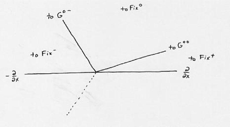
Figure 3. Rays in the $w$ Plane for Re$\,R>0$

On the other hand if Re$\,R<0$, arg$\,\xi\in(-\frac{\pi}{3},0)$. See Figure 4. Then for $\theta\in({\rm arg}\,\xi,\frac{\pi}{3})$, the ray goes to the attracting fixed point of the holonomy, and if $\theta\in(\frac{\pi}{3},\pi+{\rm arg}\,\xi)$, the ray goes to the repelling fixed point of the holonomy. The limit points of the ray with $\theta=\frac{\pi}{3}$, should map out the geodesic between these two fixed points and the vertical twist parameter will be $-\infty$.

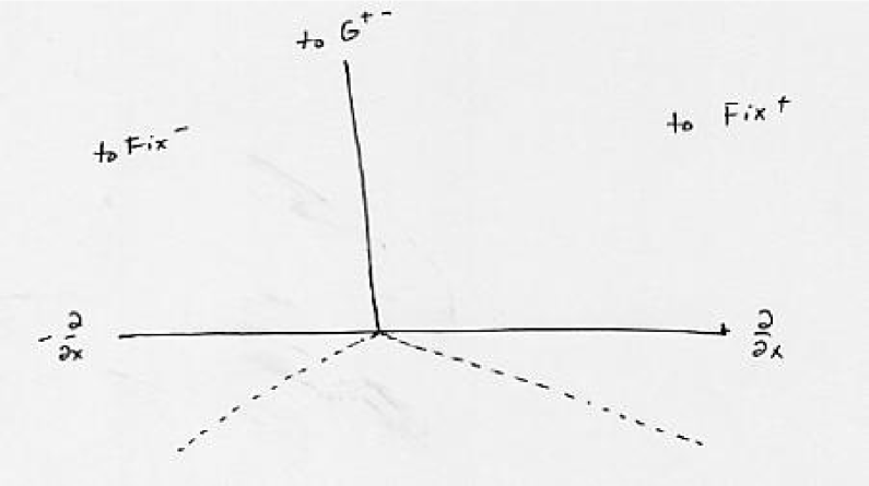
Figure 4. Rays in the $w$ Plane for Re$\,R<0$

If Re$\,R=0$, then arg$\,\xi=0$ or $\frac{\pi}{3}$, and the model breaks down. It would predict holonomy $F$ as in Proposition 8 above, which we know is incorrect.

The next few subsections will prove the $\mathbb{RP}^{2}$ structure of an end with Re$\,R\neq 0$ follow the predictions we have just made.

7.2. Perturbed linear systems

This model for the developing map is valid only near a given puncture. Recall the basic setup: We lift a neighborhood of a puncture $\{z\!:\epsilon>|z|>0\}$ on $\Sigma$ to the region in the upper half plane $\{w=x+iy\!:y>-\log\epsilon\}$. In this region we’ll use our bounds on $u$ to approximate the initial value problem for the affine sphere (8) by the explicit models computed above. As discussed in the previous subsection, it may not be useful only to consider the direction $\frac{\partial}{\partial y}$ going to infinity, but also other directions of the form (52). So for $\iota\in(0,\pi)$, introduce new coordinates $\tilde{x}=x-y\,\cot\iota$, $\tilde{y}=y\,\csc\iota$ so that

(53) $$\displaystyle\frac{\partial}{\partial\tilde{x}} = \displaystyle\frac{\partial}{\partial x}$$

(54) $$\displaystyle\frac{\partial}{\partial\tilde{y}} = \displaystyle\cos\iota\,\frac{\partial}{\partial x}+\sin\iota\,\frac{\partial}{\partial y}$$

From (8) we have the equations for $\{f,f_{w},f_{\bar{w}}\}$

(64) $$\frac{\partial}{\partial x}\left(\begin{array}[]{c}f\\ f_{w}\\ f_{\bar{w}}\\ \end{array}\right) = \left(\begin{array}[]{ccc}0&1&1\\ \frac{1}{2}e^{\psi}&\psi_{w}&Ue^{-\psi}\\ \frac{1}{2}e^{\psi}&\bar{U}e^{-\psi}&\psi_{\bar{w}}\end{array}\right)\left(\begin{array}[]{c}f\\ f_{w}\\ f_{\bar{w}}\\ \end{array}\right),$$

(74) $$\frac{\partial}{\partial y}\left(\begin{array}[]{c}f\\ f_{w}\\ f_{\bar{w}}\\ \end{array}\right) = \left(\begin{array}[]{ccc}0&i&-i\\ -i\frac{1}{2}e^{\psi}&i\psi_{w}&iUe^{-\psi}\\ i\frac{1}{2}e^{\psi}&-i\bar{U}e^{-\psi}&-i\psi_{\bar{w}}\\ \end{array}\right)\left(\begin{array}[]{c}f\\ f_{w}\\ f_{\bar{w}}\\ \end{array}\right),$$

and corresponding equations in the $\tilde{x}$ and $\tilde{y}$ coordinates. Recall the metric $e^{\psi}|dw|^{2}=e^{u}h$. The bounds on $u$ given in Proposition 5 show that in the $w$ coordinates each of $u,\,u_{w}=O(e^{-2\alpha y})$ as $y\to\infty$ for some small positive $\alpha$. Then along with the asymptotics of $U$ in (39), the definition of $h$ (35), and (53-54), we have the asymptotic result

(75) $$\frac{\partial}{\partial\tilde{x}}\mathbf{X} = \left[\mathbf{A}+\mathbf{O}(e^{-2\alpha y})\right]\mathbf{X}$$

(76) $$\frac{\partial}{\partial\tilde{y}}\mathbf{X} = \left[\mathbf{A}\,\cos\iota+\mathbf{B}\,\sin\iota+\mathbf{O}(e^{-2\alpha y})\right]\mathbf{X}$$

where $\mathbf{X}=(f,f_{w},f_{\bar{w}})^{\top}$,

$$\mathbf{A} = \left(\begin{array}[]{ccc}0&1&1\\ 2^{-\frac{2}{3}}|R|^{\frac{2}{3}}&0&-i2^{-\frac{1}{3}}R|R|^{-\frac{2}{3}}\\ 2^{-\frac{2}{3}}|R|^{\frac{2}{3}}&i2^{-\frac{1}{3}}\bar{R}|R|^{-\frac{2}{3}}&0\end{array}\right),$$

$$\mathbf{B} = \left(\begin{array}[]{ccc}0&i&-i\\ -i2^{-\frac{2}{3}}|R|^{\frac{2}{3}}&0&2^{-\frac{1}{3}}R|R|^{-\frac{2}{3}}\\ i2^{-\frac{2}{3}}|R|^{\frac{2}{3}}&2^{-\frac{1}{3}}\bar{R}|R|^{-\frac{2}{3}}&0\\ \end{array}\right).$$

In order to solve this integrable system, first solve the system in the $\tilde{y}$ direction from some initial condition—this will just be an ODE—and then solve in the $\tilde{x}$ direction (or vice versa). Consider the system

(79) $$\partial_{\tilde{x}}\mathbf{X} = \mathbf{AX}$$

(80) $$\partial_{\tilde{y}}\mathbf{X} = (\cos\iota\,\bf A+\sin\iota\,\bf B)\bf X.$$

Now change to the $\nu$ coordinate to relate these to the explicit formulas in (49). Then

$$\frac{\partial}{\partial\tilde{x}} = {\rm Re}\,\xi\,\frac{\partial}{\partial\sigma}+{\rm Im}\,\xi\,\frac{\partial}{\partial\tau}$$

$$\frac{\partial}{\partial\tilde{y}} = {\rm Re}(\xi e^{i\iota})\,\frac{\partial}{\partial\sigma}+{\rm Im}(\xi e^{i\iota})\,\frac{\partial}{\partial\tau}$$

Then the equations (79–80) become

(81) $$\partial_{\tilde{x}}\mathbf{Z} = \tilde{\mathbf{A}}\mathbf{Z}$$

(82) $$\partial_{\tilde{y}}\mathbf{Z} = \tilde{\mathbf{B}}\mathbf{Z},$$

where $\mathbf{Z}=(f,f_{\nu},f_{\bar{\nu}})^{\top}$ and

$$\tilde{\mathbf{A}} = \mathbf{P}\,\mathbf{D}\left(\rho_{1},\rho_{2},\rho_{3}\right)\,\mathbf{P}^{-1},$$

$$\tilde{\mathbf{B}} = \mathbf{P}\,\mathbf{D}\left(\mu_{1},\mu_{2},\mu_{3}\right)\,\mathbf{P}^{-1},$$

(83) $$\begin{array}[]{l@{\qquad}l}\mu_{1}=2\,{\rm Re}(\xi e^{i\iota}),&\rho_{1}=2\,{\rm Re}\,\xi,\\ \mu_{2}=2\,{\rm Re}(\xi e^{i(\iota-\frac{2\pi}{3})}),&\rho_{2}=2\,{\rm Re}(\xi e^{-i\frac{2\pi}{3}}),\\ \mu_{3}=2\,{\rm Re}(\xi e^{i(\iota+\frac{2\pi}{3})}),&\rho_{3}=2\,{\rm Re}(\xi e^{i\frac{2\pi}{3}}),\end{array}$$

(84) $$\mathbf{P}=\frac{1}{\sqrt{3}}\left(\begin{array}[]{ccc}1&1&1\\ 1&\omega&\omega^{2}\\ 1&\omega^{2}&\omega\end{array}\right).$$

Here $\mathbf{D}(\cdot,\cdot,\cdot)$ is a diagonal matrix. Also (75–76) become

(85) $$\partial_{\tilde{x}}\mathbf{Z} = \left[\tilde{\mathbf{A}}+\mathbf{O}\left(e^{-2\alpha\tilde{y}\sin\iota}\right)\right]\mathbf{Z}$$

(86) $$\partial_{\tilde{y}}\mathbf{Z} = \left[\tilde{\mathbf{B}}+\mathbf{O}\left(e^{-2\alpha\tilde{y}\sin\iota}\right)\right]\mathbf{Z}$$

Denote the perturbation terms $\mathbf{O}\left(e^{-2\alpha\tilde{y}\sin\iota}\right)$ by $\mathbf{A}^{\rm pert}$ and $\mathbf{B}^{\rm pert}$ respectively.

There is a theory, developed originally by Dunkel [12], which addresses solutions to (86) as a perturbation of (82) as $\tilde{y}\to\infty$. Below in Appendix A, we follow Levinson [25] to find a version which works with parameters. See also Hartman-Wintner [20]. It is convenient to state it in terms of an eigenbasis for $\tilde{\mathbf{B}}$.

Lemma 10.

Let $Z_{i}$ be a vector solution of the linear constant-coefficient equation (82) which has the form $e^{\mu_{i}\tilde{y}}\chi_{i}$ for a vector $\chi_{i}$. Then (86) has a solution $W_{i}$ such that

(87) $$\lim_{\tilde{y}\to\infty}\|W_{i}-Z_{i}\|e^{-\mu_{i}\tilde{y}}=0.$$

Moreover, for any solution $W$ to (86), there is a solution $Z$ to (82) satisfying estimate (87) (with $\mu_{i}$ replaced by $\mu=\lim_{\tilde{y}\to\infty}\frac{1}{\tilde{y}}\log\|W\|$).

If (86) depends continuously on a set of parameters $\tau$—i.e. if the perturbation term $\,\mathbf{B}^{\rm pert}(\tilde{y},\tau)$ continuously varies in $C^{0}([T,\infty))$ as $\tau$ varies—then $W_{i}(\tilde{y},\tau)$ is continuous in $\tau$ and the limit (87) is uniform in $\tau$.

Proof.

The exponential decay of the perturbation term in (86) are more than sufficient to apply the results in Levinson [25] to prove the first statement. The second statement follows from the first by the fact that we can choose $\{W_{i}\}$ to be a basis for the solution space of (86). We check in Appendix A that the estimates are uniform in a parameter $\tau$. ∎

Choose eigenvectors $\chi_{i}$ to be the column vectors of $\mathbf{P}$ (84). Then by the lemma we have a matrix solution $\mathbf{Z}$ to (86) so that as $\tilde{y}\to\infty$,

(88) $$\mathbf{Z}=\mathbf{P}\left(\begin{array}[]{ccc}e^{\mu_{1}\tilde{y}}+o(e^{\mu_{1}\tilde{y}})&o(e^{\mu_{2}\tilde{y}})&o(e^{\mu_{3}\tilde{y}})\\ o(e^{\mu_{1}\tilde{y}})&e^{\mu_{2}\tilde{y}}+o(e^{\mu_{2}\tilde{y}})&o(e^{\mu_{3}\tilde{y}})\\ o(e^{\mu_{1}\tilde{y}})&o(e^{\mu_{2}\tilde{y}})&e^{\mu_{3}\tilde{y}}+o(e^{\mu_{3}\tilde{y}})\end{array}\right).$$

This is enough to show that the limit of the ray in the direction $\frac{\partial}{\partial\tilde{y}}$ approaches a point on the boundary of the triangle $\mathcal{T}$, as in Table 2, with direction $\theta=\iota+{\rm arg}\,\xi.$ We also need to know, however, how this solution (88) relates to the holonomy. Equation (88) provides us with some information about a frame at infinity and how to relate it to the frame $\{f,f_{\nu},f_{\bar{\nu}}\}$.

Pick a point $p_{0}$ so that $\tilde{x}=0$ and $\tilde{y}=\tilde{y}_{0}\gg 0$. For any $\tilde{y}$, let consider the holonomy matrix $\mathbf{H}_{\tilde{y}}$ for the frame $\{f,f_{\nu},f_{\bar{\nu}}\}$ along the loop $(\tilde{x},\tilde{y})$ for $\tilde{x}\in[0,2\pi]$. Denote $\mathbf{H}_{0}=\mathbf{H}_{\tilde{y}_{0}}.$ By Section 4 above, we are free to choose initial conditions for $f$ in the initial value problem (8), at least up to a multiplicative constant, which will not essentially affect our arguments. So choose initial conditions for $f,f_{\nu},f_{\bar{\nu}}$ at $p_{0}$ so that for $\mathbf{Z}$ from (88)

(89) $$\left(f(p_{0}),f_{\nu}(p_{0}),f_{\bar{\nu}}(p_{0})\right)^{\top}=\mathbf{Z}(p_{0})=\mathbf{Z}_{0}$$

Then in a path from $(0,\tilde{y}_{0})$ to $(0,\tilde{y})$, the holonomy with respect to our frame is

(90) $$\mathbf{F}_{\tilde{y}}=\mathbf{Z}_{\tilde{y}}\mathbf{Z}_{0}^{-1}.$$

Since the connection $D$ is flat,

(91) $$\mathbf{H}_{\tilde{y}}\mathbf{F}_{\tilde{y}}=\mathbf{F}_{\tilde{y}}\mathbf{H}_{0}.$$

We also know, as in (42), $\lim_{\tilde{y}\to\infty}\mathbf{H}_{\tilde{y}}=e^{2\pi\tilde{\mathbf{A}}}$, and so as $\tilde{y}\to\infty$,

(92) $$\mathbf{H}_{\tilde{y}}=\mathbf{P}\left[\mathbf{D}(e^{2\pi\rho_{1}},e^{2\pi\rho_{2}},e^{2\pi\rho_{3}})+\mathbf{o}(1)\right]\mathbf{P}^{-1},$$

where $\rho_{i}$ are the eigenvalues of $\tilde{\mathbf{A}}$ as in (83). Compute by (88), (90), (91), and (92)

(93) $$\mathbf{H}_{0}=\mathbf{Z}_{0}\left(\begin{array}[]{ccc}e^{2\pi\rho_{1}}+o(1)&o(e^{(-\mu_{1}+\mu_{2})\tilde{y}})&o(e^{(-\mu_{1}+\mu_{3})\tilde{y}})\\ o(e^{(\mu_{1}-\mu_{2})\tilde{y}})&e^{2\pi\rho_{2}}+o(1)&o(e^{(-\mu_{2}+\mu_{3})\tilde{y}})\\ o(e^{(\mu_{1}-\mu_{3})\tilde{y}})&o(e^{(\mu_{2}-\mu_{3})\tilde{y}})&e^{2\pi\rho_{3}}+o(1)\end{array}\right)\mathbf{Z}_{0}^{-1}.$$

In the applications below, we choose the parameter $\iota$ so that two of the eigenvalues $\mu_{i}$ of $\tilde{\mathbf{B}}$ are equal to each other and greater than the remaining eigenvalue—see (83). Assume without loss of generality $\mu_{1}=\mu_{2}>\mu_{3}$. Then (92) shows

(94) $$\mathbf{H}_{0}=\mathbf{Z}_{0}\left(\begin{array}[]{ccc}e^{2\pi\rho_{1}}&0&0\\ 0&e^{2\pi\rho_{2}}&0\\ K&L&e^{2\pi\rho_{3}}\end{array}\right)\mathbf{Z}_{0}^{-1}.$$

$K$ and $L$ denote real numbers over which we have no a priori control, and this expression is with respect to the frame $\mathbf{Z}_{0}=\{f(p_{0}),f_{\nu}(p_{0}),f_{\bar{\nu}}(p_{0})\}$. Therefore, with respect to the standard frame in $\mathbb{R}^{3}$ then the holonomy is given by

(95) $$H=\left(\begin{array}[]{ccc}e^{2\pi\rho_{1}}&0&0\\ 0&e^{2\pi\rho_{2}}&0\\ K&L&e^{2\pi\rho_{3}}\end{array}\right)$$

This determines the eigenvalues of the holonomy (as in Table 1); also, $(1,0,0)$ and $(0,1,0)$ are eigenvectors corresponding to eigenvalues $e^{2\pi\rho_{1}}$ and $e^{2\pi\rho_{2}}$ respectively. (Note that $H$ acts on the right on row vectors in $\mathbb{R}^{3}$.) Therefore, projecting down to $\mathbb{RP}^{2}$, $[1,0,0]$ and $[0,1,0]$ are fixed points of the holonomy action. Each of these two fixed points is attracting, saddle, or repelling according to whether the appropriate $\rho_{j}$ ($j=1$ or 2) is numerically the largest, the middle, or the smallest of the $\{\rho_{i}\}_{i=1}^{3}$.

Recall that $f(0,\tilde{y})$ is the top row of the matrix $\mathbf{Z}$. Therefore, (88) shows that, upon projecting from $\mathbb{R}^{3}$ to $\mathbb{RP}^{2}$, $\lim_{\tilde{y}\to\infty}[f(0,\tilde{y})]=[1,1,0]$. Moreover, we have by (95)

$$\lim_{\tilde{y}\to\infty}[f(2\pi n,\tilde{y})]=[e^{2\pi n\rho_{1}},e^{2\pi n\rho_{2}},0]=\ell_{n},$$

for $n\in\mathbb{Z}$. So all these limit points $\ell_{n}$ are on a geodesic segment between $[1,0,0]$ and $[0,1,0]$. Since they are limit points of rays which go to infinity in the universal cover of $\Sigma$, and since the $\mathbb{RP}^{2}$ structure is convex, these limit points $\ell_{n}$ in $\mathbb{RP}^{2}$ must all be on the boundary $\partial\Omega$. Therefore, by convexity, the entire geodesic segment

$$\{[1,t,0]:t\in[0,\infty]\}\subset\partial\Omega.$$

We record this discussion in

Proposition 11.

Let $v_{i}$ be the standard $i^{\rm th}$ basis vector in $\mathbb{R}^{3}$, and $[v_{i}]$ the projection to $\mathbb{RP}^{2}$. Choose the parameter $\iota$ so that $\mu_{j}=\mu_{k}$ are the largest two eigenvalues of $\tilde{\mathbf{B}}$. The points $[v_{j}]$ and $[v_{k}]$ are fixed points of the holonomy. Each is attracting, repelling or saddle-type according to whether the corresponding eigenvalue of the holonomy is numerically the largest, the smallest, or the middle among $\{e^{2\pi\rho_{i}}\}_{i=1}^{3}$. The line segment

$$\{[v_{j}+tv_{k}]:t\in(0,\infty)\}$$

is in the boundary of the image of the developing map.

7.3. Hyperbolic ends: the case ${\rm Re}\,R>0$

In this case the vertical twist parameter is $\infty$.

Proposition 12.

Consider the end of the $\mathbb{RP}^{2}$ surface corresponding to $(\Sigma,U)$ with residue $R$ at the end. If Re$\,R>0$, then the vertical twist parameter of the end is $\infty$.

Proof.

If Re$\,R>0$, then choose $\xi=(2iR^{-1})^{\frac{1}{3}}$ so that arg$\,\xi\in(0,\frac{\pi}{3})$. Let $\iota=\frac{\pi}{3}-{\rm arg}\,\xi$ and $\hat{\iota}=\pi-{\rm arg}\,\xi$ so that $\theta=\iota+{\rm arg}\,\xi=\frac{\pi}{3},$ and $\hat{\theta}=\pi$.

First consider the case $\theta=\frac{\pi}{3}$. Then (83) shows that $\mu_{1}=\mu_{2}>\mu_{3}$ and $\rho_{1}>\rho_{2}>\rho_{3}$. For a value of $y\gg 0$, choose initial condition (89) for the equation (8). Proposition 11 shows that $[v_{1}]={\rm Fix}^{+}$, $[v_{2}]={\rm Fix}^{0}$ and the geodesic segment $G^{+0}$ is contained in the boundary of the image of the developing map. Moreover, the holonomy matrix with respect to the standard frame in $\mathbb{R}^{3}$ is given by (95). Note the there is as yet no a priori control over $K$ and $L$. By measuring the holonomy in the $\hat{\iota}$ direction as well, we shall see that $K$ and $L$ do vary continuously in families however.

Now for $\hat{\iota}$, $\hat{\mu}_{2}=\hat{\mu}_{3}>\hat{\mu}_{1}$ and we still have $\rho_{1}>\rho_{2}>\rho_{3}$. Therefore, again choose choose initial condition (89) for the equation (8). Note that this amounts to choosing a new frame on $\mathbb{R}^{3}$, $\{\hat{v}_{i}\}_{i=1}^{3}.$ With respect to this frame, $[\hat{v}_{2}]={\rm Fix}^{0}$ and $[\hat{v}_{3}]={\rm Fix}^{-}$. Proposition 11 shows that the geodesic segment $G^{0-}$ is in the boundary of the developing map.

By convexity, then the principal geodesic segment $G^{+-}$ must be contained in the closure $\bar{\Omega}$ of $\Omega$ the image of the developing map. We claim the open segment $G^{+-}\subset\Omega$. If on the contrary $G^{+-}\subset\partial\Omega$, then $\Omega$ is a triangle and as in Subsection 7.1, the affine metric $h$ on $\Omega$ is complete and flat. Therefore, $(\Omega,h)$ is conformally equivalent to $\mathbb{C}$. This contradicts the fact that $\Sigma$ admits a complete hyperbolic metric. Now if there were a single point of the open segment $G^{+-}$ in $\partial\Omega$, then since the endpoints ${\rm Fix}^{+}$, ${\rm Fix}^{-}\in\partial\Omega$, convexity forces all of $G^{+-}\subset\partial\Omega$, and we reach a contradiction again to prove the claim.

The discussion in Section 2 above then proves the proposition. ∎

It will be useful below to show that the holonomy matrix (95) varies continuously in families. We will determine the constants $K$ and $L$ in terms of the change of frame between the $v_{i}$ and $\hat{v}_{i}$ above.

Diagonalize (95)

$$H=\left(\begin{array}[]{ccc}1&0&0\\ 0&1&0\\ K^{\prime}&L^{\prime}&1\end{array}\right)\left(\begin{array}[]{ccc}e^{2\pi\rho_{1}}&0&0\\ 0&e^{2\pi\rho_{2}}&0\\ 0&0&e^{2\pi\rho_{3}}\end{array}\right)\left(\begin{array}[]{ccc}1&0&0\\ 0&1&0\\ -K^{\prime}&-L^{\prime}&1\end{array}\right),$$

where $K^{\prime}=K/(e^{2\pi\rho_{1}}-e^{2\pi\rho_{3}})$ and $L^{\prime}=L/(e^{2\pi\rho_{2}}-e^{2\pi\rho_{3}})$. Then in terms of the $\hat{v}_{i}$ frame,

$$\hat{H} = \left(\begin{array}[]{ccc}e^{2\pi\rho_{1}}&\hat{K}&\hat{L}\\ 0&e^{2\pi\rho_{2}}&0\\ 0&0&e^{2\pi\rho_{3}}\end{array}\right)$$

$$= \left(\begin{array}[]{ccc}1&\hat{K}^{\prime}&\hat{L}^{\prime}\\ 0&1&0\\ 0&0&1\end{array}\right)\left(\begin{array}[]{ccc}e^{2\pi\rho_{1}}&0&0\\ 0&e^{2\pi\rho_{2}}&0\\ 0&0&e^{2\pi\rho_{3}}\end{array}\right)\left(\begin{array}[]{ccc}1&-\hat{K}^{\prime}&-\hat{L}^{\prime}\\ 0&1&0\\ 0&0&1\end{array}\right),$$

where $\hat{K}^{\prime}=\hat{K}/(e^{2\pi\rho_{2}}-e^{2\pi\rho_{1}})$ and $\hat{L}^{\prime}=\hat{L}/(e^{2\pi\rho_{3}}-e^{2\pi\rho_{1}})$.

Denote by $Q$ the change of frame in $\mathbb{R}^{3}$ between the $v_{i}$ and the $\hat{v}_{i}$. Then $H=Q\hat{H}Q^{-1}$. Since the eigenvalues $\{e^{2\pi\rho_{i}}\}$ are distinct, there must exist real constants $\omega_{i}\neq 0$ so that

$$\left(\begin{array}[]{ccc}1&0&0\\ 0&1&0\\ K^{\prime}&L^{\prime}&1\end{array}\right)\left(\begin{array}[]{ccc}\omega_{1}&0&0\\ 0&\omega_{2}&0\\ 0&0&\omega_{3}\end{array}\right)=Q\left(\begin{array}[]{ccc}1&\hat{K}^{\prime}&\hat{L}^{\prime}\\ 0&1&0\\ 0&0&1\end{array}\right)$$

Let $Q=(Q^{i}_{j})$. The previous equation forces $Q^{2}_{1}=Q^{2}_{3}=0$, and the free parameters are determined by $Q$:

$$\begin{array}[]{c}\displaystyle\hat{K}^{\prime}=-\frac{Q^{1}_{2}}{Q^{1}_{1}},\quad\hat{L}^{\prime}=-\frac{Q^{1}_{3}}{Q^{1}_{1}},\quad K^{\prime}=\frac{Q^{3}_{1}}{Q^{1}_{1}},\quad L^{\prime}=\frac{Q^{3}_{2}Q^{1}_{1}-Q^{3}_{1}Q^{1}_{2}}{Q^{1}_{1}Q^{2}_{2}},\\ \displaystyle\omega_{1}=Q^{1}_{1},\quad\omega_{2}=Q^{2}_{2},\quad\omega_{3}=\frac{Q^{3}_{3}Q^{1}_{1}-Q^{3}_{1}Q^{1}_{3}}{Q^{1}_{1}}.\end{array}$$

Note the last row implies $Q^{1}_{1},Q^{2}_{2}\neq 0$. $Q$ is determined by the initial conditions $\mathbf{Z}_{0}$ and $\hat{\mathbf{Z}}_{0}$ from (89) to the initial value problem (8). Explicitly, Proposition 1 shows that $Q=\hat{\mathbf{Z}}_{0}^{-1}\mathbf{Z}_{0}$. $\mathbf{Z}_{0}$ and $\hat{\mathbf{Z}}_{0}$ come from Lemma 10. Therefore, Lemma 10 and Proposition 24 imply the parameters $K,L,\hat{K},\hat{L}$ vary continously in families.

Proposition 13.

The holonomy matrix (95) constructed above varies continuously for families of equations as long as the perturbation term $\mathbf{B}^{\rm pert}(y,\tau)$ satisfies the hypotheses of Lemma 10.

Remark.

Here is a more geometric interpretation of the preceeding Proposition and its proof. The proposition allows us to control the $\mathbb{RP}^{2}$ coordinates of the developing map of a degenerating family. In other words, it allows us to control the gauge. Developing along rays for the parameter $\iota$ allow us to control the line segment $G^{+0}$, and similarly for the parameter $\hat{\iota}$, we control the line segment $G^{0-}$, up to a change of gauge $Q$ which varies continuously. Any automorphism of $\mathbb{RP}^{2}$ which fixes $G^{+0}\cup G^{0-}$ must be trivial, and so the proposition follows.

7.4. Hyperbolic ends: the case ${\rm Re}\,R<0$

In this case, the vertical twist parameter is $-\infty$.

Proposition 14.

On an end of $(\Sigma,U)$ with residue $R$ so that Re$\,R<0$, the principal geodesic line segment of the holonomy action around this end is in the boundary of the image of the developing map. The vertical twist parameter for this end is $-\infty$.

Proof.

If Re$\,R<0$, then choose $\xi=(2iR^{-1})^{\frac{1}{3}}$ so that arg$\,\xi\in(-\frac{\pi}{3},0)$. Let $\iota=\frac{\pi}{3}-{\rm arg}\,\xi$ so that $\theta=\frac{\pi}{3}.$ Then (83) shows that $\mu_{1}=\mu_{2}>\mu_{3}$ and $\rho_{1}>\rho_{3}>\rho_{2}$. Proposition 11 then implies that $[1,0,0]={\rm Fix}^{+}$ and $[0,1,0]={\rm Fix}^{-}$, and that the geodesic segment between them, $G^{+-}$, is contained in the boundary of the image of the developing map. The discussion in Section 2 above then implies the vertical twist parameter is $-\infty$. ∎

7.5. Quasi-hyperbolic ends

For Re$\,R=0$, $R\neq 0$, Table 1 shows the holonomy type of the end is quasi-hyperbolic. This completely determines the structure of the end.

Proposition 15.

Let $S$ be a properly convex $\mathbb{RP}^{2}$ surface with an end with quasi-hyperbolic holonomy. If $\Omega\subset\mathbb{RP}^{2}$ is the universal cover, then the end of $S$ has boundary given by the push-down of a geodesic segment in $\partial\Omega$ whose endpoints are the two fixed points of the holonomy action.

Proof.

Lift the holonomy action to $\mathbf{SL}(3,\mathbb{R})$ and choose coordinates $(x_{1},x_{2},x_{3})$ in $\mathbb{R}^{3}$ so that the holonomy matrix is of the form

$$\gamma=\left(\begin{array}[]{ccc}\alpha_{1}&1&0\\ 0&\alpha_{1}&0\\ 0&0&\alpha_{3}\end{array}\right).$$

Here $\alpha_{i}>0$, $\alpha_{1}^{2}\alpha^{3}=1$, and $\alpha_{1}\neq\alpha_{3}$. Consider the case $\alpha_{1}>\alpha_{3}$. The two fixed points of the holonomy are a repelling fixed point Fix${}^{-}=[0,0,1]$, and Fix${}^{P}=[1,0,0]$. There are also two geodesic lines preserved by the holonomy given by $L=\{x_{2}=0\}$, which connects the two fixed points and on which the action is hyperbolic; and $L^{\prime}=\{x_{3}=0\}$, on which the action is parabolic.

Pick a point $p=[x_{1},x_{2},1]\in\Omega\setminus(L\cup L^{\prime})$. Then $p_{n}=\gamma^{n}p$ satisfies $\lim_{n\to\infty}p_{n}={\rm Fix}^{P}$, $\lim_{n\to-\infty}p_{n}={\rm Fix}^{-}$. The convexity of $\Omega$ implies that one of the two geodesic segments between Fix^- and Fix^P must be contained in $\bar{\Omega}$. If $x_{2}>0$, then it is the segment $G^{\rm pos}=\{[t,0,1]:t>0\}$, and if $x_{2}<0$, then it is the segment $G^{\rm neg}=\{[t,0,1]:t<0\}$. Now we claim that this segment $G^{\rm pos}$ or $G^{\rm neg}$ must be in the boundary $\partial\Omega$. Without loss of generality, assume $x_{2}>0$. Then if a neighborhood of any point in $G^{\rm pos}$ is contained in $\Omega$, then $\Omega$ contains a point with $x_{2}<0$, and therefore $\bar{\Omega}$ contains $G^{\rm neg}$ as well, and so $\partial\Omega$ contains the whole line $L$. This contradicts the fact that $\Omega$ is strictly convex. See Figure 5. The case $\alpha_{1}<\alpha_{3}$ is similar. ∎

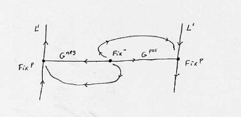
Figure 5. The Dynamics of Quasi-Hyperbolic Holonomy

7.6. Parabolic ends

If the residue $R=0$, Table 1 shows the holonomy type of the end is parabolic. As in the quasi-hyperbolic case above, the holonomy’s being parabolic completely determines the structure of the end.

Proposition 16.

Let $S$ be a properly convex $\mathbb{RP}^{2}$ surface with an end with parabolic holonomy. Assume the fundamental group $\pi_{1}(S)\neq\mathbb{Z}$. If $\Omega\subset\mathbb{RP}^{2}$ is the universal cover of $S$, then the end of $S$ has boundary (as a set) given by the push-down of the single fixed point of the holonomy action, which is in $\partial\Omega$.

Proof.

Lift the holonomy action to $\mathbf{SL}(3,\mathbb{R})$. Choose coordinates in $(x^{1},x^{2},x^{3})$ of $\mathbb{R}^{3}$ so that the holonomy matrix is

$$\gamma=\left(\begin{array}[]{ccc}1&1&0\\ 0&1&1\\ 0&0&1\end{array}\right).$$

The only fixed point is ${\rm Fix}=[1,0,0]$. Also, there is a single line preserved by the holonomy action given by the line $L=\{x^{3}=0\}$. The holonomy is parabolic along $L$. For any point $p\in\Omega$ and $p_{n}=\gamma^{n}p$, then we have $p_{n}\to{\rm Fix}$ for $n\to\pm\infty$. Therefore, $\rm{Fix}\in\bar{\Omega}$. Since the holonomy acts on $\Omega$ without fixed points, $\rm{Fix}\in\partial\Omega$.

For a domain $\Omega$ on which $\gamma$ acts, there are two ends of the cylindrical quotient $\Omega/\langle\gamma\rangle$. See Figure 6. Call the end which develop to Fix the small end, and the other the large end. We want to rule out the large end. Notice that the holonomy action $\gamma^{n}$ takes the part of $\partial\Omega$ associated with the large end to all of $\partial\Omega\setminus\{{\rm Fix}\}$.

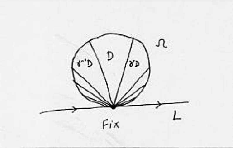
Figure 6. Parabolic Holonomy

Assume that our end develops to the large end of $\Omega/\langle\gamma\rangle.$ As in Subsection 6.1 above, fix a basepoint $p\in S$ near the end in question, and consider a path $P$ going from $p$ to the end which doesn’t leave a fixed cylindrical neighborhood $N$ of the end. Fix a fundamental domain $D\in\tilde{S}$ which contains a lift $\tilde{P}$ of the path $P$. We may assume that dev$(\tilde{P})$ has a limit point $r\in\partial\Omega$. Since we have dev$(\tilde{P})$ is contained in the large end, we may assume $r\neq{\rm Fix}$. By the action of $\gamma^{n}$ on the large end, a simple continuity argument, along with Figure 6, shows that the closure in $\mathbb{RP}^{2}$ of $\bigcup_{n}{\rm dev}(\gamma^{n}D)$ contains all of $\partial\Omega$, and also includes a neighborhood in $\bar{\Omega}$ of $\partial\Omega\setminus\{{\rm Fix}\}$.

Now consider an element $\gamma^{\prime}\in\pi_{1}(S)\setminus\langle\gamma\rangle$, and the corresponding holonomy $H={\rm hol}(\gamma^{\prime})\in\mathbf{PGL}(3,\mathbb{R})$. Then we may assume, by perturbing the path $P$ if necessary, that $H(r)\neq{\rm Fix}$. But of course $H(r)\in\partial\Omega$. Also, $H(r)$ is the limit point of the path $\gamma^{\prime}\tilde{P}$, where we consider $\gamma^{\prime}$ as the path starting at $\tilde{p}\in\tilde{S}$ and covering an appropriate loop. But this then contradicts the fact that $\overline{\bigcup_{n}{\rm dev}(\gamma^{n}D)}$ contains a neighborhood in $\bar{\Omega}$ of $\partial\Omega\setminus\{{\rm Fix}\}$. ∎

8. The boundary of the moduli space

8.1. Regular 3-differentials

The material in this subsection is well known. I would like to thank Michael Thaddeus, Ravi Vakil and Richard Wentworth for explaining some of it to me. A basic reference for the algebraic theory is the book of Harris and Morrison [harris-morrison]. A good summary of the analytic techniques used here is contained in Wolpert [32]. We only give a sketch of the arguments.

Consider the Deligne-Mumford compactification $\overline{\mathcal{M}}_{g}$ of the moduli space of Riemann surfaces of genus $g\geq 2$ and also $\overline{\mathcal{M}}_{g,1}$ the compactification of the of the moduli space of genus-$g$ Riemann surfaces with one marked point $p$. Let $\mathcal{F}\!:\overline{\mathcal{M}}_{g,1}\to\overline{\mathcal{M}}_{g}$ be the forgetful map. In this context, $\overline{\mathcal{M}}_{g,1}$ is the universal curve over $\overline{\mathcal{M}}_{g}$. These moduli spaces are only V-manifolds (smooth Deligne-Mumford stacks). We will describe complex coordinates on the sense of V-manifolds: in general, for each point $x$ in the moduli space there is a chart given by the quotient of an open set in $\mathbb{C}^{N}$ by a finite group $G$ of biholomorphisms. (For details of V-manifolds, see Baily [1].) Charts in Teichmüller space provide these V-manifold charts near $x\in\mathcal{M}_{g}$. (We describe below coordinate charts near $x\in\overline{\mathcal{M}}_{g}\setminus\mathcal{M}_{g}$.) The group $G$ is given by the group of automorphisms of the curve $\mathcal{F}^{-1}(x)$ over the point $x$. (In the case $g=2$ with no marked point, the group $G$ is instead the quotient of the group of automorphisms of the curve by the automorphism group of the generic curve, which is generated by the hyperelliptic involution.)

At a point $x\in\mathcal{M}_{g}$, consider the curve $C_{0}$ over $x$. In Teichmüller space $\mathcal{T}_{g}$ consisting of $3g-3$ Beltrami differentials $\nu_{i}$. For $s=(s^{i})\in\mathbb{C}^{3g-3}$ small, then $\|s^{i}\nu_{i}\|_{L^{\infty}}<1$ and thus there is a quasiconformal map homeomorphism $C_{0}$ to $C_{s}$ with Beltrami differential $s^{i}\nu_{i}$. Then $s$ form local $C^{\infty}$ V-manifold coordinates around $x\in\mathcal{M}_{g}$. Note $s$ is not a holomorphic coordinate system.

Each point $x\in\overline{\mathcal{M}}_{g}\setminus\mathcal{M}_{g}$, represents a Riemann surface with nodes. In other words, at each point $p$ in our curve $C$ over $x$ has a neighborhood of the form either $\{z:|z|<K\}$ or $\{(z,z^{\prime}):zz^{\prime}=0,|z|<K,|z^{\prime}|<K\}$. Let $n$ be the number of nodes. Let $C^{\rm reg}$ be the smooth part of $C$, which is formed by removing the $n$ nodes. $C^{\rm reg}$ is a possibly disconnected noncompact Riemann surface. $C^{\rm reg}$ may be smoothly compactified to $\tilde{C}$ by adding $2n$ points $\{p_{i},q_{i}\}$. $\tilde{C}$ is the normalization of $C$. A natural analytic map from $\tilde{C}$ to $C$ identifies each pair $(p_{i},q_{i})$ to a single point to form each node. $C$ must be stable: i.e. $C$ has only finitely many automorphisms; equivalently $C^{\rm reg}$ admits a conformal complete hyperbolic metric.

A natural deformation of $C$ consists of plumbing the nodes, in which we replace each node $\{zz^{\prime}=0\}$ by the smooth neck $\{zz^{\prime}=t\}$. There is a nice overview of the plumbing construction in Wolpert [32]. A neighborhood of the $i^{\rm th}$ node is for local coordinates $z_{i},z_{i}^{\prime}$

(98) $$N_{i}=\{(z_{i},z_{i}^{\prime}):z_{i}z_{i}^{\prime}=0,|z_{i}|<K,|z_{i}^{\prime}|<K\}.$$

For a complex parameter $t_{i}:|t_{i}|<K^{2}$, we replace $N_{i}$ by the smooth cylinder $N_{i}^{t_{i}}=\{(z_{i},z_{i}^{\prime}):z_{i}z_{i}^{\prime}=t_{i},|z_{i}|<K,|z_{i}^{\prime}|<K\}$. It is clear that for $t$=$(t_{i})$

$$C_{t}=\left[C\setminus\left(\cup_{i}N_{i}\right)\right]\bigsqcup\left(\cup_{i}N_{i}^{t_{i}}\right)$$

patches together complex-analytically to make $\Sigma_{t}$ smooth on a neighborhood of each $\overline{N_{i}^{t_{i}}}$. These $t_{i}$ form $n$ complex V-manifold coordinates over $\overline{\mathcal{M}}_{g}$.

In addition, Wolpert [35, Lemma 1.1] has shown there is a real-analytic family of Beltrami differentials $\nu(s)$ on $C^{\rm reg}$ parametrized by $s$ in a neighborhood of the origin in $\mathbb{C}^{3g-3-n}$ so that the induced quasiconformal maps $\zeta^{\nu(s)}\!:C^{\rm reg}\to C^{\rm reg}_{s}$ preserve the cusp coordinate up to multiplying by a rotation $e^{i\theta_{s}}$. Form $C_{s}$ by completing $C^{\rm reg}_{s}$ by reattaching the corresponding nodes. For the $n$ nodes and $t\in\mathbb{C}^{n}$ small, we perform the plumbing construction as above with respect to the cusp coordinates on each $C_{s}$ to form a family $C_{s,t}$ of curves. Then $(s,t)$ form a real-analytic V-manifold coordinate chart of $\overline{\mathcal{M}}_{g}$ near a nodal curve. For each fixed $s$, the $t$ coordinates are complex-analytic.

There are similar coordinates on the universal curve $\overline{\mathcal{M}}_{g,1}$. The idea is to treat the marked point $p$ as a puncture. As above, by Lemma 1.1 in [35], in $\mathcal{M}_{g,1}$, there is a real-analytic family of Beltrami differentials $\nu(s)$ for $s$ in a neighborhood of 0 in $\mathbb{C}^{3g-3}$ so that the quasiconformal maps $\zeta^{\nu(s)}$ preserve a canonical complex coordinate neighborhood $U$ of $p\in C_{0}$. Then $p$ may move complex-analytically in $U$ so that $(s,p)$ form a real-analytic V-manifold coordinate chart of $\mathcal{M}_{g,1}$, and for each fixed $s$, the $p$ coordinate is complex-analytic.

It is straightforward to combine the construction in the last two paragraphs in the case of a nodal curve $C$ with $n$ nodes over a point in $\overline{\mathcal{M}}_{g}\setminus\mathcal{M}_{g}$ and a point $p\in C^{\rm reg}$. Then we have real-analytic coordinates $(s,p,t)$ with $s\in U\subset\mathbb{C}^{3g-3-n}$, $t\in U^{\prime}\subset\mathbb{C}^{n}$, and $p\in U^{\prime\prime}\subset C^{\rm reg}_{s,t}$ so that for $s$ fixed, the coordinates $(p,t)$ are complex-analytic.

In the remaining case of a nodal curve $C$ with $p$ at a node is more subtle. First of all, having $p$ equal to a node is technically not allowed in the Deligne-Mumford compactification. Let the node in $C$ be represented by $zz^{\prime}=0$. Then if $p$ is the point of the node $\{z=z^{\prime}=0\}$, this configuration is not stable. Instead introduce a sphere $\mathbb{CP}^{1}$ attached to $\tilde{C}$ by one point $r\in\mathbb{CP}^{1}$ to $\{z=0\}$ and by another point $r^{\prime}\in\mathbb{CP}^{1}\setminus\{r\}$ to $\{z^{\prime}=0\}$. This amounts to having a sphere “bubbling” to separate the existing node into two pieces and having the sphere attached by nodes at $r,r^{\prime}$ to each piece. See Figure 7 (in the case the node separates the curve into two parts $C^{1}$ and $C^{2}$). Then $p$ is allowed to be any point in $\mathbb{CP}^{1}\setminus\{r,r^{\prime}\}$. However, since the sphere with three marked points $p,r,r^{\prime}$ has no automorphisms, we may collapse the $\mathbb{CP}^{1}$ and identify this configuration canonically with the configuration of the point $p$ equal to the node $\{z=z^{\prime}=0\}$. Then $p$ is no longer a smooth complex coordinate, since it must vary in a singular curve at the singularity. Instead consider the plumbing variety $\{zz^{\prime}=t\}\subset\mathbb{C}^{3}$ for $z,z^{\prime},t$ near 0 and $t=t_{1}$. $(z,z^{\prime})$ are natural complex coordinates for the plumbing variety—see e.g. [32]. Then as above there is a complex $3g-3-n$ dimensional family of real-analytic coordinates $s$ corresponding to quasiconformal maps which preserve the complex coordinates near the nodes. $(s,z,z^{\prime},t_{2},\cdots,t_{n})$ form a real-analytic coordinate neighborhood in $\overline{\mathcal{M}}_{g,1}$ so that for each fixed $s$, $(z,z^{\prime},t_{2},\cdots,t_{n})$ are complex-analytic coordinates.

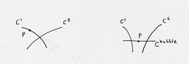
Figure 7. $\overline{\mathcal{M}}_{g,1}$ near a Node

Let $\rho$ be a positive integer. On any Riemann surface with local coordinate $z$, a section $U$ of $K^{\rho}$ with a pole of order $\rho$ at $p=\{z=0\}$ has a residue $R^{U}_{p}$, which is the the coefficient of the $\left(\frac{dz}{z}\right)^{\rho}$ term in the Laurent series of $U$. It is easy to check $R^{U}_{p}$ does not depend on the complex coordinate $z$. Over a curve $C$ with $n$ nodes formed by pairing up $n$ pairs of points $(p_{i},q_{i})$ in $\tilde{C}$, the space of regular $\rho$-differentials over $C$ is

$$\left\{U\in H^{0}(\tilde{C},K_{\tilde{C}}^{\rho}\Pi_{i}([p_{i}]^{\rho}[q_{i}]^{\rho})):R^{U}_{p_{i}}=(-1)^{\rho}R^{U}_{q_{i}}\quad\forall\,i=1,\dots,n\right\}.$$

In other words these are sections of $K^{\rho}$ over $\tilde{C}$ with poles of order $\rho$ allowed at $p_{i},q_{i}$ so that the residues match up appropriately on either side of each node. We are interested in the case $\rho=3$ of regular 3-differentials and we denote the sheaf of regular 3-differentials over $C$ as $K^{3,{\rm reg}}_{C}$.

Let $\mathcal{K}^{3}$ be the line bundle over $\overline{\mathcal{M}}_{g,1}$ whose fiber over a pointed curve $(C,p)$ is the vector space $K^{3,{\rm reg}}_{C}(p)$ the fiber of the regular 3-differentials over $C$ at $p$. It straightforward that this forms a holomorphic line bundle over $\overline{\mathcal{M}}_{g,1}$, except possibly in the situation of a nodal curve $C$ in which the marked point $p$ is equal to a node. Recall the situation above: we separate the node and place a bubble $\mathbb{CP}^{1}$ in between attached to the local normalization $\tilde{C}^{\rm loc}$ at points $r$ and $r^{\prime}$. $p$ is any other point in $\mathbb{CP}^{1}$. Call this new curve $C^{\rm bubble}$. Then any regular 3-differential on $C^{\rm bubble}$ has residues

$$R_{z=0}=-R_{r}\quad\mbox{and}\quad R_{z^{\prime}=0}=-R_{r^{\prime}}.$$

Now $\dim_{\mathbb{C}}H^{0}(\mathbb{CP}^{1},K^{3}[r]^{3}[r^{\prime}]^{3})=1$, and the residues satisfy $R_{r}=-R_{r^{\prime}}$. Thus $R_{z=0}=-R_{z^{\prime}=0}$. So $\mathcal{K}^{3}$ at this point has a stalk naturally corresponding to the residues at the node $p=\{z=z^{\prime}=0\}$.

Now a local trivialization of $\mathcal{K}^{3}$ near the point in $\overline{\mathcal{M}}_{g,1}$ corresponding to $(C,p)$ is given in terms of the coordinates $z,z^{\prime}$ of the plumbing variety. For $z\neq 0$, $z^{\prime}\neq 0$, let

$$T=\left(\frac{dz}{z}\right)^{3}=-\left(\frac{dz^{\prime}}{z^{\prime}}\right)^{3},$$

and $T$ is well-defined except at the node. Then $T$ extends over the node $\{z=z^{\prime}=0\}$ to a local trivialization so that at the node $T$ has residues $R^{T}_{z=0}=1$ and $R^{T}_{z^{\prime}=0}=-1$. This is simply in terms of the coordinates on the plumbing variety $z,z^{\prime}$. In general we take

(99) $$T=c(s)\left(\frac{dz}{z}\right)^{3}=-\,c(s)\left(\frac{dz^{\prime}}{z^{\prime}}\right)^{3},$$

where the scalar $c(s)$ depends only real-analytically on $s$. We may take $c(0)=1$. This factor appears because the $s$ coordinates on $\overline{\mathcal{M}}_{g,1}$ are only real-analytic with respect to the underlying complex structure.

Now push forward the sheaf $\mathcal{K}^{3}$ by the map $\mathcal{F}\!:\overline{\mathcal{M}}_{g,1}\to\overline{\mathcal{M}}_{g}$ to form a sheaf $\mathcal{S}=K^{3}_{\overline{\mathcal{M}}_{g,1}/\overline{\mathcal{M}}_{g}}$ over $\overline{\mathcal{M}}_{g}$. In particular, since the cohomology $H^{i}(C,K^{3,{\rm reg}})=\{0\}$ for all $i>0$, and ${\rm dim}\,H^{0}(C,K^{3,{\rm reg}})=5g-5$, a theorem of Grauert [18] shows that $\mathcal{S}$ is a (V-manifold) vector bundle over $\overline{\mathcal{M}}_{g}$. See Masur [27, Prop. 4.2] or Fay [13] for details.

In particular, in a neighborhood of point corresponding to a Riemann surface with nodes in $\overline{\mathcal{M}}_{g}$, there is a holomorphic frame of regular 3-differentials.

Proposition 17.

A basis for the analytic toplogy on the total space of $\mathcal{S}=\mathcal{F}_{*}(\mathcal{K}^{3})$ consists of neighborhood of $(C,U)$, where $C$ is a curve with $n$ nodes and $U\in H^{0}(C,K^{3,{\rm reg}})$ consists of pairs $(C_{s,t},U_{s,t})$ so that $(s,t)$ is close to zero in $\mathbb{C}^{3g-3}$, and $U_{s,t}$ is close to $U$ in the following way: Let the plumbing collars be represented by $\{z_{i}z^{\prime}_{i}=t_{i}:|z_{i}|,|z^{\prime}_{i}|<K\}$. Outside the plumbing collars, we require

$$\left|\frac{U_{s,t}}{(dz^{\nu(s)})^{3}}-\frac{U}{dz^{3}}\right|<\epsilon$$

for $z^{\nu(s)}$ the local conformal coordinate on $C_{s,t}$ determined by the quasiconformal map for a local coordinate $z$ on $C$. Inside the plumbing collars $|z_{i}|,|z_{i}^{\prime}|<K$, we require

$$\left|\frac{z_{i}^{3}}{dz_{i}^{3}}\left(U_{s,t}-U\right)\right|<\epsilon.$$

Proof.

This is proved in the above paragraphs. In particular the last statement follows from the trivialization (99) of $\mathcal{K}^{3}$. We remark that since the cusp coordinate $z_{i}^{\nu(s)}=e^{i\theta_{s}}z_{i}$ by Wolpert’s Lemma 1.1 in [35], $\frac{(dz_{i}^{\nu(s)})^{3}}{(z_{i}^{\nu(s)})^{3}}=\frac{dz_{i}^{3}}{z_{i}^{3}}$ for $z_{i}$ inside the collar neighborhood. ∎

Remark.

Fay [13] and Yamada [36] produce a more explicit asymptotic expansion for a basis of regular 1-differentials on a degenerating family of Riemann surfaces, and Masur [27] does the same for regular 2-differentials. The same techniques should apply to the present case of regular 3-differentials as well. Such a specific result is not needed in this paper.

We use this characterization to describe a degenerating family of pairs $(C_{\tau},U_{\tau})$, which approach a pair $(C_{0},U_{0})$ of a nodal curve $C_{0}$ and a regular 3-differential $U_{0}$ on $C_{0}$. In general, the parameter $\tau=\tau(s,t_{1},\dots,t_{n})$. For notational simplicity, we focus on the case $\tau=t_{1}=t$ the plumbing parameter of the first node. Given a noded surface $C_{0}$ and a degenerating family $C_{t}$ determined by plumbing coordinates $zz^{\prime}=t$, a regular 3-differential $U_{0}$ on $C_{0}$ may be described as a limit of holomorphic 3-differentials $U_{t}$ on $C_{t}$. Recall (98). Then

$$U_{0}|_{z^{\prime}=0} = \sum_{m=-3}^{\infty}a_{m}z^{m}dz^{3}$$

$$U_{0}|_{z=0} = \sum_{m=-3}^{\infty}b_{m}(z^{\prime})^{m}(dz^{\prime})^{3}$$

where $b_{-3}=-a_{-3}$. Then by Proposition 17 we may define on the collar neighborhood $\{z:|z|\in[\frac{|t|}{K},K]\}\subset C_{t}$

$$U_{t}=\sum_{m=-\infty}^{\infty}a_{m}(t)z^{m}dz^{3},$$

where $a_{m}(t)$ is a continuous function of $t$ so that for $m\geq-3$, $a_{m}(0)=a_{m}$, and for $m\leq-3$, $a_{m}(t)=-t^{-m-3}b_{-m-6}(t)$, where $b_{n}(t)$ is continuous in $t$ and $b_{n}(t)=b_{n}$ for $n\geq-3$. (To make $U_{t}$ a holomorphically varying family, we may choose $a_{m}$, $b_{m}$ to vary holomorphically in $t$ up to the matter of a branch cover of degree 2. See e.g. Masur [27].)

It is useful to compute in terms of more symmetric coordinates. For some choice of branch of $\log t$, let $\ell$ be the quasi-coordinate function given by

(100) $$\ell=\log z-{\textstyle\frac{1}{2}}\log t=-\log z^{\prime}+{\textstyle\frac{1}{2}}\log t,$$

and let $\mu=\rm{Re}\,\ell$. Then we have

(101) $$U_{t}=\left(-\sum_{n=1}^{\infty}b_{n-3}(t)t^{\frac{n}{2}}e^{-n\ell}+a_{-3}(t)+\sum_{n=1}^{\infty}a_{n-3}(t)t^{\frac{n}{2}}e^{n\ell}\right)d\ell^{3}.$$

Note that we may include the parameters $(s,t_{2},\dots,t_{n})$. In this case the coefficients $b_{m}$ and $a_{m}$ vary continuously in these parameters as well. Also, let $\ell_{s,t}=\log z^{\nu(s)}-\frac{1}{2}\log t$ for $z^{\nu(s)}$ the complex coordinate on $C_{s,t}$ given by the quasi-conformal map determined by $\nu(s)$.

8.2. Holonomy of necks approaching a QH end

Recall that at a QH end, the residue $R=a_{-3}(0)\neq 0$. In this case, we have on either side of the node, the model metric is given by (35), and which is the same for residue $R$ and $-R$. These are flat cylindrical metrics of the same radius which can simply be glued together in the plumbing construction. For each $t$ small, we modify the cylindrical metric to be

(102) $$h_{t}=2^{\frac{1}{3}}|a_{-3}(t)|^{\frac{2}{3}}|d\ell|^{2}.$$

(Recall $|d\ell|^{2}=\frac{|dz|^{2}}{|z|^{2}}=\frac{|dz^{\prime}|^{2}}{|z^{\prime}|^{2}}$.) Note that again, for simplicity, we repress the dependence of $h_{t}$ on the other variables $(s,t_{2},\dots,t_{n})$, in which $h_{t}$ varies continuously. We may assume that the plumbing parameter $t$ satisfies $|t|<c^{2}$, where $c$ is the constant as in (36), so that the Ansatz metric is flat for $|z|,|z^{\prime}|<c$. (Note we can choose a uniform $c$ for a neighborhood of 0 in $t$ as long as $a_{-3}(t)$ is bounded away from 0.)

We will modify the barriers constructed in Subsection 5.2 above to show that as $t\to 0$, the solution $u$ to (31) will go to zero on the neck which is being pinched to the node. Although the cylindrical metrics fit together well, the barriers must be modified.

Our barriers will be functions only of $\mu={\rm Re}\,\ell$. For $S=S(\mu)$, use (101) so that equation (37) becomes

(103) $$L(S)=2^{-\frac{1}{3}}|a_{-3}(t)|^{-\frac{2}{3}}S^{\prime\prime}-2e^{S}+2e^{-2S}\left[1+O(|t|^{\frac{1}{2}}e^{\mu})+O(|t|^{\frac{1}{2}}e^{-\mu})\right].$$

We need $L(S)\geq 0$ for a lower barrier and $L(S)\leq 0$ for an upper barrier.

Modify the barrier only in a neighborhood of the loop

$$\mathcal{L}_{t}=\{|z|=|z^{\prime}|=|t|^{\frac{1}{2}}\}=\{\mu=0\},$$

where $\mu={\rm Re}\,\ell$. We may do this because outside a neighborhood $|z|,|z^{\prime}|<K$, the original barriers suffice—outside this neighborhood, $U_{0}$ changes to $U_{t}$ continuously, and all the choices made in constructing the barriers in Subsection 5.2 can easily be made to accommodate this small perturbation.

Recall our upper and lower barriers in Subsection 5.2 are of the form $\pm\beta|z|^{2\alpha}$, for $\beta\gg 0$ and $\alpha>0$ small. We may adjust these constants so that the same $\beta$ and $\alpha$ are valid for both upper and lower barriers on both sides of the puncture. On the plumbed surface choose our upper barrier $S_{t}$ to be equal to

$$S_{t}=\left\{\begin{array}[]{l@{\quad\mbox{for}\quad}l}\beta|t|^{\alpha}e^{2\alpha\mu}&\mu\in\left[1,\log K-\frac{1}{2}\log|t|\right]\\ I_{t}(\mu)&\mu\in[-1,1]\\ \beta|t|^{\alpha}e^{-2\alpha\mu}&\mu\in\left[-\log K+\frac{1}{2}\log|t|,-1\right]\end{array}\right.$$

Notice that for the first and third lines of this definition are respectively $\beta|z|^{2\alpha}$ and $\beta|z^{\prime}|^{2\alpha}$. The middle part $I_{t}(\mu)$ is a $C^{2}$ interpolation between these two. Explicitly, we may take $I_{t}(\mu)$ to be the even fourth-order polynomial in $\mu$ so that $S_{t}$ is $C^{2}$ at $\mu=\pm 1$. In other words, for $Q=S_{t}(1)=S_{t}(-1)=\beta|t|^{\alpha}e^{2\alpha}$,

$$I_{t}(\mu) = Q\left[(1-{\textstyle\frac{5}{4}}\alpha+{\textstyle\frac{1}{2}}\alpha^{2})+({\textstyle\frac{3}{2}}\alpha-\alpha^{2})\mu^{2}+(-{\textstyle\frac{1}{4}}\alpha+{\textstyle\frac{1}{2}}\alpha^{2})\mu^{4}\right],$$

$$I_{t}^{\prime\prime}(\mu) = \alpha Q\left[(3-2\alpha)+(-3+6\alpha)\mu^{2}\right].$$

Therefore, we claim we can choose $\alpha$ independent of $t$ so that for $t$ near 0, $I_{t}(\mu)>0$ and $L(I_{t})\leq 0$ for $\mu\in[-1,1]$. As in (38), rewrite (103) as

$$L(I_{t}) = \left(2^{-\frac{1}{3}}|a_{-3}(t)|^{-\frac{2}{3}}I_{t}^{\prime\prime}-3I_{t}\right)+\left(2e^{-2I_{t}}-2e^{I_{t}}+3I_{t}\right)$$

$${}+e^{-2I_{t}}\left[O(|t|^{\frac{1}{2}}e^{\mu})+O(|t|^{\frac{1}{2}}e^{-\mu})\right]$$

$L(I_{t})\leq 0$ follows: $2e^{-2I_{t}}-2e^{I_{t}}+3I_{t}<0$ for if $I_{t}>0$. For $\alpha$ small, $Q$ dominates the perturbation terms $O(|t|^{\frac{1}{2}}e^{\mu})$ and $O(|t|^{\frac{1}{2}}e^{-\mu})$; therefore, the first term dominates the last and $L(I_{t})\leq 0$. This shows that $S_{t}$ is an upper barrier for (31) on the region $\mu={\rm Re}\,\ell\in[-1,1]$.

For $|\mu|\in[1,\log K-\frac{1}{2}\log|t|]$, Proposition 17 shows $\|U_{t}\|_{h_{t}}^{2}\to\|U\|_{h}^{2}$ uniformly in in the plumbing variety coordinates $z,z^{\prime}$ as $t\to 0$. By our choice of $h_{t}$ in (102),

$$\|U_{t}\|_{h_{t}}^{2}\leq 2+C|z|+C^{\prime}|z^{\prime}|$$

for constants $C,C^{\prime}$. Since this is true for all $t$, we may choose $C,C^{\prime}$ uniformly in $t$. Then the last term in (38) is dominated by the first for $\alpha$ small, $\beta$ large, and $(z,z^{\prime})$ close to 0, where these choices may be made independently of $t$. Then $L(S_{t})\leq 0$ for $|\mu|\in[1,\log K-\frac{1}{2}\log|t|]$.

Therefore, $S_{t}$ is an upper barrier for (31). Essentially the same arguments show that near $\{|\mu|\leq\log K-\frac{1}{2}\log|t|\}$, $-S_{t}$ forms a lower barrier for solutions to (31) with data $(C_{t}^{\rm reg},U_{t},h_{t})$, and as in Subsection 5.2, there is a constant $B_{t}$ so that a lower barrier is equal to $-S_{t}$ inside the plumbing collars and $B_{t}$ outside. $B_{t}$ depends continuously on $t$.

Again following Subsection 5.2, the maximum principle says that there is a bounded solution $u_{t}$ to (31) on $C_{t}^{\rm reg}$ so that $|u_{t}|\leq S_{t}$ for $|z|,|z^{\prime}|<K$. Note that as $t\to 0$, $S_{t}\to 0$ on a neighborhood of the loop $\mathcal{L}_{t}$. The geometry is still uniformly bounded in this case; so we still have the bound on $u_{t}$ and $\nabla u_{t}$ as in Proposition 5. Then let $\mathbf{A}_{t}$ be the holonomy around the loop $\mathcal{L}_{t}$ with respect to the frame $\{f,f_{w},f_{\bar{w}}\}$ as in (40). Orient $\mathcal{L}_{t}$ counterclockwise in the $z$ coordinate. Then Lemma 6 still holds and we have as in the proof of Proposition 7

Proposition 18.

As $t\to 0$, the eigenvalues of the holonomy along $\mathcal{L}_{t}$ approach $e^{2\pi\lambda_{i}}$ for $\lambda_{i}$ the roots, with multiplicity, of formula (41).

In terms of the other parameters $(s,t_{2},\dots,t_{n})$, the Ansatz metric $h_{s,t}$ and the upper and lower barriers vary continuously. One thing to note is that for $s$ small, Wolpert’s Beltrami differential $\nu(s)$ is close to 0 and supported away from the collar neighborhoods. Therefore, the complex structure and hyperbolic metric on $C^{\rm reg}_{s}$ are close to that on $C^{\rm reg}_{0}$. Then on $C^{\rm reg}_{s,t}$, we take $h_{s,t}$ to be the hyperbolic metric on $C^{\rm reg}_{s,0}$ outside the collar neighborhoods and modify the metrics $h_{t}$ as in (36,102) inside the collar neighborhoods only.

8.3. Vertical twist parameters of a family

Recall that if ${\rm Re}\,R>0$, then the vertical twist parameter of the end is $+\infty$. Theorem 6 part (2) will follow from Proposition 13 above. First note that in a neighborhood in the total space of $\mathcal{K}^{3}$, by the previous subsection, there are uniform bounds on $\|U_{\tau}\|$ on each Riemann surface $C_{\tau}^{\rm reg}$ for $\tau$ near 0. Also, there are uniform barriers of the form $\beta|z_{i}|^{2\alpha}$ and $\beta|z^{\prime}_{i}|^{2\alpha}$ in each plumbing collar, and uniform constant barriers in on the rest of $C_{\tau}$. Then we may bootstrap as in Lemma 4 to find uniform estimates on the third covariant derivatives of $u_{\tau}$ the solution to (31) for data $(C_{\tau}^{\rm reg},U_{\tau},h_{\tau})$. Therefore, by Ascoli-Arzela, a subsequence of $u_{\tau}$ converges in $C^{2}$ (determined by covariant derivatives of the metric) to a solution $\tilde{u}$ of (31) for data $(C^{\rm reg},U,h)$. By Proposition 3, $\tilde{u}=u$ and thus there are $C^{2}$ estimates for $u_{\tau}$ approaching $u$. In particular, by (74), the perturbation matrix $\mathbf{B}^{\rm pert}_{\tau}$ from (76) varies continuously in $\tau$ in the plumbing collar.

More specifically, in terms of the $\ell$ coordinate in a collar neighborhood as in the previous subsection, $\mathbf{B}^{\rm pert}_{\tau}$ is uniformly continuous in $\tau$ and satisfies

$$|\mathbf{B}^{\rm pert}_{\tau}|\leq\beta|t|^{\alpha}e^{2\alpha\mu}\quad\mbox{for }\mu\in[1,\log K-{\textstyle\frac{1}{2}}\log|t|],$$

where $t=t(\tau)$. In terms of the $y$ coordinate,

$$|\mathbf{B}^{\rm pert}_{\tau}|\leq\beta e^{-2\alpha y}\quad\mbox{for }y\in[-\log K,-1-{\textstyle\frac{1}{2}}\log|t|].$$

We have similar bounds in the $\tilde{y}$ coordinates (54). Now for $t$ small, replace $\mathbf{B}^{\rm pert}_{\tau}$ by

$$\mathbf{B}^{\rm cutoff}_{\tau}=\left\{\begin{array}[]{r@{\mbox{ for }}l}\mathbf{B}^{\rm pert}_{\tau}&y\leq-1-\frac{1}{2}\log|t|\\ f(x,y,\tau)&y>-1-\frac{1}{2}\log|t|\end{array}\right.$$

so that $\mathbf{B}^{\rm cutoff}_{\tau}$ satisfies the hypotheses of Lemma 10. Then for $t=t(\tau)$ small, the solution to (76) satisfies the asymptotic bounds (88), and moreover the $o(e^{\mu_{i}\tilde{y}})$ terms are uniform in $\tau$ as $t(\tau)\to 0$. Therefore, as in Subsection 7.3 above, we may fix a large initial value of $y$, say $y_{0}$, independent of $\tau$, and the solutions to the equations (using $\mathbf{B}^{\rm cutoff}$) in the two directions determined by $\iota$ and $\hat{\iota}$ give solutions which approach the geodesic line segments $G^{+0}$ and $G^{0-}$ respectively. (Notice that in these cases by (83) $\tilde{\mathbf{B}}$ and $\mathbf{B}^{\rm cutoff}$ satisfy the hypotheses of Proposition 24.) Now for the actual $\mathbb{RP}^{2}$ structure determined by $(C_{\tau}^{\rm reg},U_{\tau})$, we must take our original perturbation term $\mathbf{B}^{\rm pert}$. But for $y\leq-1-\frac{1}{2}\log|t|$, the solutions are the same by uniqueness of solutions to ODEs. Since $y_{0}$ is fixed and the bound $-1-\frac{1}{2}\log|t|\to\infty$ as $t\to 0$, there are, as $t\to 0$, two regions of the developing map which approach the geodesic line segments $G^{+0}$ and $G^{0-}$ respectively. The only way this can happen is if the vertical twist parameter is approaching $+\infty$ as $\tau\to 0$.

In the case of a node with ${\rm Re}R_{i}<0$, there is not as much information concerning the holonomy maps, but we do know that the residue of the other half of the node has positive real part, and from the point of view of the residue with ${\rm Re}R_{i}>0$, the vertical twist parameter approaches $+\infty$. Therefore, the vertical twist parameter from the opposite point of view shrinks to $-\infty$.

8.4. Holonomy of necks approaching a parabolic end

Recall from Section 5 that the Ansatz and the barrier for a parabolic end (one for which the residue $R_{i}=0$) is of quite a different form. The Ansatz metric is the hyperbolic metric, and the upper and lower barriers near the puncture are both constants. We are free to make these constants larger in norm by the methods above, and thus we can assure that the barriers on either side of the node are the same constant, and thus patch together naturally as the node is plumbed.

The metric, on the other hand, must be smoothed across the plumbed node. It is crucial that the curvature still be negative and bounded away from 0 and $-\infty.$ For this purpose, we recall the plumbing metric in Wolpert [34]. See also Wolf-Wolpert [31].

Proposition 19.

[34] Let $C_{0}$ be a stable nodal Riemann surface, and let $C_{t}$ be the plumbed surface as above. On the plumbing collar $\{zz^{\prime}=t\}$ for $|z|,|z^{\prime}|\leq K$, there is a metric $h_{t}$ which is equal to the hyperbolic metric on $C_{0}$ outside the plumbing collar(s), and satisfies

(104) $$h_{t}=\left\{\begin{array}[]{l@{\mbox{ for }}l@{\mbox{ i.e., }}l}\frac{4|dz|^{2}}{|z|^{2}(\log|z|^{2})^{2}}&|z|\in[\frac{2K}{3},K]&|z^{\prime}|\in[\frac{|t|}{K},\frac{3|t|}{2K}]\\ \left(\frac{\pi}{\log|t|}\csc(\frac{\pi\log|z|}{\log|t|})\frac{|dz|}{|z|}\right)^{2}&|z|\in[\frac{3|t|}{K},\frac{K}{3}]&|z^{\prime}|\in[\frac{3|t|}{K},\frac{K}{3}]\\ \frac{4|dz^{\prime}|^{2}}{|z^{\prime}|^{2}(\log|z^{\prime}|^{2})^{2}}&|z|\in[\frac{|t|}{K},\frac{3|t|}{2K}]&|z^{\prime}|\in[\frac{2K}{3},K]\\ \end{array}\right.$$

and smoothly interpolated for $|z|,|z^{\prime}|\in[\frac{K}{3},\frac{2K}{3}]$. The curvature $\kappa_{t}$ on $(C_{t},h_{t})$ satisfies

$$\|\kappa_{t}+1\|_{C^{0}}\leq\gamma|t|^{\delta}$$

for uniform constants $\gamma,\delta>0$.

Remark.

For our purposes, we may take the model grafting in Section 3.4.MG of Wolpert [34]. We do not need to use the more complicated (and accurate) grafting procedures in Section 3.4.CG of [34] or in [31].

Lemma 20.

There is a constant $\delta^{\prime}$ so that if $|t|\leq\delta^{\prime}$ and $\|U_{t}\|_{h_{t}}\leq\mathcal{K}$ for a constant $\mathcal{K}$ independent of $t$, then there is a constant $\mathcal{K}^{\prime}$ independent of $t$ so that solution $u_{t}$ to (31) satisfies $|u_{t}|\leq\mathcal{K}^{\prime}$.

Proof.

In Subsection 5.2, the upper and lower barriers for (31) on the curve $C_{0}$ is equal to a constant in the neighborhood of the node in question (note that the constants may be adjusted on either side of the node to be equal). A constant $M_{t}>0$ is an upper barrier of (31) if

$$4e^{-2M_{t}}\|U_{t}\|_{h_{t}}^{2}-2e^{M_{t}}-2\kappa_{t} \leq 0\quad\mbox{i.e.,}$$

$$4\|U_{t}\|_{h_{t}}^{2}-2E_{t}^{3}-2\kappa_{t}E_{t}^{2} \leq 0,$$

for $E_{t}=e^{M_{t}}$. It is easy to see that $E_{t}$ may be chosen independently of $t$ given that $\|U_{t}\|_{h_{t}}$ is bounded independently of $t$, and (by Proposition 19) $\kappa_{t}$ satisfies $-k^{\prime}\leq\kappa_{t}\leq-k$ for positive constants $k,k^{\prime}$. Similar considerations apply for the lower barrier. ∎

Proposition 21.

Let $\mathbf{A}_{t}$ be the holonomy around the loop $\mathcal{L}_{t}=\{|z|=|z^{\prime}|=|t|^{\frac{1}{2}}\}$ with respect to the frame $\{f,f_{w},f_{\bar{w}}\}$ as in (40). Orient $\mathcal{L}_{t}$ counterclockwise in the $z$ coordinate. If there are uniform positive constants $\delta^{\prime},C$ so that for $|t|\leq\delta^{\prime}$,

(105) $$\sup_{|z|\in[\frac{K}{|t|},K]}\left|\frac{z^{3}(U_{t}-U_{0})}{dz^{3}}\right|\left|\log|t|\right|^{3}\leq C,$$

then $\mathbf{A}_{t}$ is continuous in $t$ and

$$\lim_{t\to 0}\mathbf{A}_{t}=\left(\begin{array}[]{ccc}0&1&1\\ 0&0&0\\ 0&0&0\end{array}\right).$$

Proof.

Recall

$$\mathbf{A}_{t}=\left(\begin{array}[]{ccc}0&1&1\\ \frac{1}{2}e^{\psi}&\psi_{w}&Ue^{-\psi}\\ \frac{1}{2}e^{\psi}&\bar{U}e^{-\psi}&\psi_{\bar{w}}\end{array}\right).$$

for $z=e^{iw}$, $\psi=\phi+u$, $h_{t}=e^{\phi}|dw|^{2}$, and $w=x+iy$. Note we suppress the dependence on $t$. The continuity in $t$ follows from the fact that $u_{t}$ and its derivatives vary continuously in $t$ by standard elliptic regularity arguments, as in the first paragraph of Subsection 8.3 above. (In particular, it is easy to check that the metric (104) has bounded geometry on a uniformly large neighborhood of $\mathcal{L}_{t}$.) Also near $\mathcal{L}_{t}$,

$$\phi=2\log\left(\frac{-\pi}{\log|t|}\right)-2\log\sin\left(\frac{-\pi y}{\log|t|}\right).$$

On $\mathcal{L}_{t}$, $y=-\frac{1}{2}\log|t|$, and so

$$e^{\phi}=\left(\frac{\pi}{\log|t|}\right)^{2},\quad\mbox{and}\quad\phi_{w}=0.$$

Moreover, by Lemma 20, $|u|\leq\mathcal{K}^{\prime}$. We still have Lemma 4, which shows

$$|u_{w}|\leq\mathcal{K}^{\prime\prime}e^{\frac{\phi}{2}}=\mathcal{K}^{\prime\prime}\frac{\pi}{\left|\log|t|\right|}$$

Finally, the assumption (105) on $U$, the fact that $U_{0}$ has residue 0, and the uniform bound on $u$ shows as $t\to 0$, $Ue^{-\psi}\to 0$ on $\mathcal{L}_{t}$. Similarly, all the other entries in the second and third rows of $\mathcal{A}_{t}$ go to zero. ∎

Then as above in Subsection 6.2, the eigenvalues of the holonomy around the loop $\mathcal{L}_{t}$ all approach 1 as $t\to 0$.

In terms of more general paths $(C_{\tau},U_{\tau})$ in $\mathcal{S}$, calculating the limiting holonomy depends on having uniform $C^{0}$ estimates on $u$ independent of $\tau$. The model metric on $C_{\tau}$ is simply the hyperbolic metric on $C_{s(\tau),0}$ outside the collar neighborhoods and may be modified as above in each collar neighborhood. Note that the complex structure and hyperbolic metrics on $C_{s(\tau),0}$ vary continuously as in Wolpert’s Lemma [35]. In a neighborhood of a singular curve $C_{0}$ with $n$ nodes, consider V-manifold coordinates $(t_{1},\dots,t_{n},s)$ in $\overline{\mathcal{M}}_{g}$ near $C_{0}$. Let $U_{0}$ have residue 0 at $k$ of the $n$ nodes. Without loss of generality, assume these nodes correspond to the plumbing parameters $(t_{1},\dots,t_{k})$. Then

Proposition 22.

For $(C_{\tau},U_{\tau})$ a continuous path in $\mathcal{S}$, if in addition there are uniform positive constants $\delta,C$ so that for $|\tau|\leq\delta$, $U_{\tau}$ satisfies

(106) $$\sup_{|z_{i}|,|z_{i}^{\prime}|\in[\frac{K}{|t_{i}|},K]}\left|\frac{z_{i}^{3}(U_{\tau}-U_{0})}{dz_{i}^{3}}\right|\left|\log|t_{i}|\right|^{3}\leq C$$

for $t_{i}=t_{i}(\tau)$ and for all $i\in\{1,\dots,k\}$, then the eigenvalues of the holonomy around each neck are continuous in $\tau$.

Given a holomorphic frame $\{\Psi^{1},\dots,\Psi^{5g-5}\}$ of the vector bundle $\mathcal{S}\to\overline{\mathcal{M}}_{g}$, we have the following

Corollary 23.

Write $U_{\tau}=a_{j}(\tau)\Psi^{j}$, where $a=(a_{j})\in\mathbb{C}^{5g-5}$ and $\Psi^{j}$ represents the element of $H^{0}(C_{\tau},K^{3,{\rm reg}})$ corresponding to the frame. Then if there is a uniform $C$ so that

$$|[a(\tau)-a(0)](\log|t_{i}|)^{3}|\leq C\quad\mbox{for }i=1,\dots,k,$$

then the eigenvalues of the holonomy around each neck are continuous in $\tau$.

8.5. Results

We record the results of the previous subsections in

Theorem 6.

Consider a continuous path of pairs $(C_{\tau},U_{\tau})$, where the possibly nodal curve $C_{\tau}$ represents a point in $\overline{\mathcal{M}}_{g}$ and $U_{\tau}$ is a holomorphic section of $K^{3,{\rm reg}}_{C_{\tau}}$ so that $C_{0}$ is a nodal curve with $n$ nodes. For each node, pick one side from which to measure the residue. For any curve $C_{\tau}$ which approximates $C_{0}$ by pinching a neck to form the node, this amounts to choosing an orientation for any loop around that neck. Then $U_{0}$ is a cubic differential with residue $R_{i}$ for each node.

1. If all the residues $R_{i}\neq 0$, then the eigenvalues of the holonomy around each neck which is pinched to the node continuously approach the eigenvalues of the holonomy around the punctures of the complete Riemann surface $C_{0}^{\rm reg}$ as in Table 1. The same is true if we have some residues $R_{1},\dots,R_{k}=0$ as long as $U_{\tau}$ satisfies the addition set of bounds (106).

2. Still assume (106) for all nodes with 0 residue. Consider a node whose residue $R_{i}$ satisfies ${\rm Re}\,R_{i}\neq 0$. Then the vertical twist parameter along this neck $N$ approaches $\pm\infty$, the sign agreeing with the sign of the ${\rm Re}\,R_{i}$. In fact, if ${\rm Re}\,R_{i}>0$, there is a continuous path of points $p_{\tau}\in\overline{\mathcal{M}}_{g,1}$ so that $p_{\tau}\in C_{\tau}$ and $p_{\tau}$ avoids all nodes, and a continuously varying choice of $\mathbb{RP}^{2}$ coordinate chart near $p_{\tau}$ in the $\mathbb{RP}^{2}$ surface $S_{\tau}$ determined by $(C_{\tau}^{\rm reg},U_{\tau})$. The holonomy matrix with respect to these $\mathbb{RP}^{2}$ coordinates of the neck $N$ has fixed points Fix${}^{0}_{\tau}$, Fix${}^{+}_{\tau}$ and Fix${}^{-}_{\tau}$ which vary continuously with $\tau$. If we fix coordinates on $\mathbb{RP}^{2}$ so that Fix${}^{0}_{\tau}$, Fix${}^{+}_{\tau}$ and Fix${}^{-}_{\tau}$ are fixed, then the image $\Omega_{\tau}$ of the developing map satisfies

   $$\lim_{\tau\to 0}\Omega\tau\supset T,$$

   where $T$ is the principal triangle whose vertices are the fixed points. (In other words for all points $q\in T$, there is a constant $\delta$ so that if $|\tau|\leq\delta$, then $q\in\Omega_{\tau}$.)

Remark.

We expect that the technical restrictions on the continuous paths $(C_{\tau},U_{\tau})$ in the case $R_{i}=0$ can be removed.

8.6. The $\mathbb{RP}^{2}$ structure on a degenerating neck

By the definition of regular 3-differentials, it is worthwhile to compare the $\mathbb{RP}^{2}$ holonomy of two punctures in $\Sigma=C^{\rm reg}$ equipped with cubic differentials with residues $R$ and $-R$, as these will naturally be identified in the nodal curve $C$. Recall that the eigenvalues of the holonomy are given by $e^{2\pi\lambda_{i}}$, where $\lambda_{i}$ are the roots of (41). If we replace $R$ by $-R$ in (41), then the roots $\lambda_{i}$ become $-\lambda_{i}$. In terms of the holonomy matrix, at least in the hyperbolic case, the holonomy matrix satisfies $H_{-R}=H_{R}^{-1}$. We may think of this as the same holonomy viewed from opposite orientations, which is natural: the holonomy is given in terms of loops which go counterclockwise around each puncture, and if want to glue two such punctures together, the two loops will be oriented in opposite directions.

In the case of parabolic and quasi-hyperbolic holonomies, the holonomy is the only invariant we have of the end, but there is also the vertical twist parameter for hyperbolic ends. Assume Re$\,R>0$. Then the vertical twist parameter for this end is $+\infty$, while the vertical twist parameter with the corresponding end with residue $-R$ will be $-\infty$. Again this is to be expected. We may imagine a family of surfaces degenerating in a way that their vertical twist parameters become infinite. Then measured from one side, (vertical twist parameter going to $+\infty$) the piece of the developing map glued along the principal geodesic is becoming larger and larger until it becomes the entire principal triangle. From the other side (for which the vertical twist parameter goes to $-\infty$), the glued piece of the developing map becomes smaller and smaller until it vanishes and the boundary is simply the principal geodesic. See Section 2.

Appendix A Linear almost constant-coefficient systems with parameters

Proposition 24.

Consider a system of linear differential equations

(107) $$\partial_{y}X(s,y)=(c(s)B+R(s,y))X(s,y),$$

where $y\geq T$, $s$ is a set of parameters, $B=\mathbf{D}(\mu_{1},\dots,\mu_{n})$ is a constant $n\times n$ diagonal matrix, the scalar factor $c(s)$ is continuous, and the matrix entries of the error term $R(s,y)$ are smooth and $L^{1}$ in $y$ and vary in $s$ so that for all $i,j$, the map $s\mapsto R^{j}_{i}(s,y)$ is continuous to $L^{1}([T,\infty))$.

Then there exist $n$ linearly independent solutions $X^{(k)}(s,y)$ to (107) so that for $\{v_{k}\}$ the standard basis on $\mathbb{R}^{n}$,

$$X^{(k)}(s,y)=e^{c(s)\mu_{k}y}v_{k}+e^{c(s)\mu_{k}y}b(s,y),$$

and $X^{(k)}(s,y)$ is continuous in $(s,y)$, $\lim_{y\to\infty}|b(s,y)|=0$ uniformly in $s$ for $s$ in a bounded region.

Remark.

If in addition (as we have above), there are uniform positive constants $C,\gamma$ so that $|R^{j}_{i}(s,y)|\leq Ce^{-\gamma y}$, then we can replace $c(s)B$ by a continuous family $B(s)$ of diagonal matrices, and moreover a more precise error bound on $X^{(k)}-e^{B(s)\mu_{k}y}v_{k}$ holds. Since we do not need this better result, we do not prove it here.

Proof.

We follow the treatment in Levinson [25, pp. 115–117]. The only additional thing to prove is the continuity of solutions in $s$. Assume $\mu_{i}$ the eigenvalues of $B$ are arranged so that

$${\rm Re}\,\mu_{1}\geq{\rm Re}\,\mu_{2}\geq\cdots\geq{\rm Re}\,\mu_{n}.$$

Fix $k\in\{1,\dots,n\}$. Choose $q=q(k)$ so that

$${\rm Re}\,\mu_{k}={\rm Re}\,\mu_{q}>{\rm Re}\,\mu_{q+1}$$

(or $q=n$ if this is impossible). Define $X_{i}^{0}=\delta_{ik}e^{c(s)\mu_{k}y}$, and define $X_{i}^{m}$ recursively by

$$\begin{array}[]{rclr}X^{m+1}_{i}(s,y)&=&\displaystyle\delta_{ik}e^{c(s)\mu_{k}y}-\int_{y}^{\infty}e^{\mu_{i}(y-\sigma)}R_{i}^{j}(s,\sigma)X^{m}_{j}(s,\sigma)\,d\sigma&(i\leq q),\\ X^{m+1}_{i}(s,y)&=&\displaystyle\int_{a}^{y}e^{\mu_{i}(y-\sigma)}R_{i}^{j}(s,\sigma)X^{m}_{j}(s,\sigma)\,d\sigma&(i>q).\end{array}$$

The index $j$ is summed from $1$ to $n$, but no sum is taken over $i$. If for some $m$, $X_{i}^{m}=X_{i}^{m+1}$, then this $X_{i}^{m}$ solves (107) as long as the integrals involved converge absolutely.

Now it is clear that $X_{i}^{0}$ is continuous in $(s,y)$. By induction, the same is true for $X_{i}^{m}$ for all $m$. As in [25],

$$|X^{m+1}_{i}-X^{m}_{i}|\leq 2^{-m}\left|e^{c(s)\mu_{k}y}\right|,$$

and so the series (for $X^{-1}_{i}=0$)

$$X_{i}=\sum_{m=-1}^{\infty}(X^{m+1}_{i}-X^{m}_{i})$$

is majorized by a geometric series. Also $X=(X_{i})$ solves (107). In particular, $X^{m}$ converges locally uniformly to $X$ in $(s,y)$ and $X$ is continuous in $(s,y)$. This $X$ is the $X^{(k)}$ in the proposition.

The bound on the error term in [25] is of the form

$$|b_{i}(s,y)|\leq e^{-\epsilon y}|R|_{L^{1}}+2\sum_{j}\int_{\frac{y}{2}}^{\infty}|R^{j}_{i}(s,\sigma)|\,d\sigma$$

for a uniform positive constant $\epsilon$. This shows the required uniform bound on $|b(s,y)|$. The rest of the proposition follows as in [25]. ∎

References

- [1] W. L. Baily. On the imbedding of V-manifolds in projective space. American Journal of Mathematics, 79:403–430, 1957.
- [2] E. Calabi. Complete affine hyperspheres I. Instituto Nazionale di Alta Matematica Symposia Mathematica, 10:19–38, 1972.
- [3] S.-Y. Cheng and S.-T. Yau. Differential equations on Riemannian manifolds and their geometric applications. Communications on Pure and Applied Mathematics, 28:333–354, 1975.
- [4] S.-Y. Cheng and S.-T. Yau. On the regularity of the Monge-Ampère equation . Communications on Pure and Applied Mathematics, 30:41–68, 1977.
- [5] S.-Y. Cheng and S.-T. Yau. Complete affine hyperspheres. part I. The completeness of affine metrics. Communications on Pure and Applied Mathematics, 39(6):839–866, 1986.
- [6] S. Choi. Convex decompositions of real projective surfaces. I: -annuli and convexity. Journal of Differential Geometry, 40(1):165–208, 1994.
- [7] S. Choi. Convex decompositions of real projective surfaces. II: Admissible decompositions. Journal of Differential Geometry, 40(2):239–283, 1994.
- [8] S. Choi. Convex decompositions of real projective surfaces. III: For closed and nonorientable surfaces. Journal of the Korean Mathematical Society, 33(4):1139–1171, 1996.
- [9] S. Choi and W. M. Goldman. Convex real projective structures on closed surfaces are closed. Proceedings of the American Mathematical Society, 118(2):657–661, 1993.
- [10] S. Choi and W. M. Goldman. The classification of real projective structures on compact surfaces. Bulletin (New Series) of the American Mathematical Society, 34(2):161–171, 1997.
- [11] M.-R. Darvishzadeh and W. M. Goldman. Deformation spaces of convex real projective and hyperbolic affine structures. Journal of the Korean Mathematical Society, 33:625–638, 1996.
- [12] O. Dunkel. Regular singular ponts of a system of homogeneous linear differential equations of the first order. Proceedings of the American Academy of Arts and Sciences, 38:341–370, 1902–03.
- [13] J. D. Fay. Theta Functions on Riemann Surfaces, volume 352 of Lecture Notes in Mathematics. Springer-Verlag, 1973.
- [14] D. Gilbarg and N. Trudinger. Elliptic Partial Differential Equations of Second Order. Springer-Verlag, 1983.
- [15] W. M. Goldman. The symplectic nature of the fundamental groups of surfaces. Advances in Mathematics, 54:200–225, 1984.
- [16] W. M. Goldman. Convex real projective structures on compact surfaces. Journal of Differential Geometry, 31:791–845, 1990.
- [17] W. M. Goldman. The symplectic geometry of affine connections on surfaces. Journal für die reine und agnewandte Mathematik, 407:126–159, 1990.
- [18] H. Grauert. Ein Theorem der analytischen Garbentheorie und die Modulräume komplexer Strukturen. Pub. Math. IHES, 5:233–292, 1960.
- [19] P. Hartman. Ordinary Differential Equations. Wiley, 1964.
- [20] P. Hartman and A. Wintner. Asymptotic integrations of linear differential equations. American Journal of Mathematics, 77:45–86, 1955.
- [21] N. J. Hitchin. The self-duality equations on a Riemann surface. Proceedings of the London Mathematical Society, 55(3):59–126, 1987.
- [22] N. J. Hitchin. Lie groups and Teichmüller space. Topology, 31(3):449–473, 1992.
- [23] H. C. Kim. The symplectic global coordinates on the moduli space of real projective structures. Journal of Differential Geometry, 53(2):359–401, 1999.
- [24] F. Labourie. in Proceedings of the GARC Conference in Differential Geometry, Seoul National University, Fall 1997, 1997.
- [25] N. Levinson. The asymptotic nature of solutions of linear systems of differential equations. Duke Mathematical Journal, 15:111–126, 1948.
- [26] J. C. Loftin. Affine spheres and convex manifolds. American Journal of Mathematics, 123(2):255–274, 2001.
- [27] H. Masur. The extension of the Weil-Petersson metric to the boundary of Teichmüller space. Duke Mathematical Journal, 43(3):623–635, 1976.
- [28] K. Nomizu and T. Sasaki. Affine Differential Geometry: Geometry of Affine Immersions. Cambridge University Press, 1994.
- [29] C.-P. Wang. Some examples of complete hyperbolic affine -spheres in . In Global Differential Geometry and Global Analysis, volume 1481 of Lecture Notes in Mathematics, pages 272–280. Springer-Verlag, 1991.
- [30] M. Wolf. Infinite energy harmonic maps and degeneration of hyperbolic surfaces in moduli space. Journal of Differential Geometry, 33:487–539, 1991.
- [31] M. Wolf and S. Wolpert. Real analytic structures on the moduli space of curves. American Journal of Mathematics, 114:1079–1102, 1992.
- [32] S. Wolpert. Geometry of the Weil-Petersson completion of Teichmüller space. preprint, June 2002.
- [33] S. Wolpert. On the Weil-Petersson geometry of the moduli space of curves. American Journal of Mathematics, 107:969–997, 1985.
- [34] S. Wolpert. The hyperbolic metric and the geometry of the universal curve. Journal of Differential Geometry, 31(2):417–472, 1990.
- [35] S. Wolpert. Spectral limits for hyperbolic surfaces II. Inventiones Mathematicae, 108(1):91–129, 1992.
- [36] A. Yamada. Precise variational formulas for Abelian differentials. Kodai Mathematical Journal, 3:114–143, 1980.