A phase transition and stochastic domination in Pippenger’s probabilistic failure model for Boolean networks with unreliable gates

Abstract

We study Pippenger’s model of Boolean networks with unreliable gates. In this model, the conditional probability that a particular gate fails, given the failure status of any subset of gates preceding it in the network, is bounded from above by some $\varepsilon$. We show that if a Boolean network with $n$ gates is selected at random according to the Barak-Erdős model of a random acyclic digraph, such that the expected edge density is $cn^{-1}\log n$, and if $\varepsilon$ is equal to a certain function of the size of the largest reflexive, transitive closure of a vertex (with respect to a particular realization of the random digraph), then Pippenger’s model exhibits a phase transition at $c=1$. Namely, with probability $1-o(1)$ as $n\to\infty$, we have the following: for $0\leq c\leq 1$, the minimum of the probability that no gate has failed, taken over all probability distributions of gate failures consistent with Pippenger’s model, is equal to $o(1)$, whereas for $c>1$ it is equal to $\exp\left(-\frac{c}{e(c-1)}\right)+o(1)$. We also indicate how a more refined analysis of Pippenger’s model, e.g., for the purpose of estimating probabilities of monotone events, can be carried out using the machinery of stochastic domination.

Keywords and Phrases:

Boolean network, Lovász local lemma, phase transition, probabilistic method, random graph, reliable computation with unreliable components, stochastic domination.

AMS Subject Classification (2000):

82B26; 94C10; 60K10; 05C20; 05C80

1 Introduction

The study of phase transitions in combinatorial structures, such as random graphs [3, 7, 25] is a subject at the intersection of statistical physics, theoretical computer science, and discrete mathematics [2, 6, 8, 9, 29, 30, 37, 40]. The key idea behind this study is that large combinatorial structures can be thought of as systems consisting of many locally interacting components, in direct analogy to the kinds of systems within the purview of statistical mechanics. A phase transition, then, is a phenomenon that takes place in certain kinds of such systems in the limit of an infinite number of components, and corresponds qualitatively to a change in some global (macroscopic) parameter of the system as the local parameters of the components are varied.

Boolean networks with gates subject to probabilistic failures fall naturally into the category of systems just described. The possibility of a phase transition arises here, for instance, when one associates a probability of failure with each gate of such a network, and then looks at the maximum of the probability that the network deviates (outputs an incorrect result), taken over all possible assignments of inputs to the network, in the limit of an infinite number of gates. The theory of Boolean networks with unreliable gates can be traced back to the seminal work of von Neumann [32], who considered the simplest case, namely when each gate in the network fails with fixed probability $\varepsilon$ independently of all other gates — we will refer to this set-up as the $\varepsilon$-independent failure model. Von Neumann’s initial work was developed further by Dobrushin and Ortyukov [11, 12], Pippenger [33], Feder [16], Pippenger, Stamoulis, and Tsitsiklis [36], and Gács and Gál [19], to name just a few. (It should be mentioned that in Ref. [36] the authors pointed out several technical flaws of [11] and presented their own proof of a weaker result; Gács and Gál [19] later developed methods to recover the full result claimed in [11].) Now we will summarize relevant notions and ideas in a more or less narrative fashion; the requisite details will be supplied in Section 2.

One of the key results obtained by von Neumann [32] was the following: if the probability $\varepsilon$ of gate failure is sufficiently small, then any Boolean function can be computed by a network of unreliable gates such that the probability of error is bounded by a constant independent of the function being computed. On the other hand, since in this model a Boolean network is no more reliable than its last gate, the probability of error can get arbitrarily close to one if the probability of gate failure is sufficiently large. (This is, in fact, one possibility for a phase transition in Boolean networks with unreliable gates, which we have alluded to in the preceding paragraph.)

However, as pointed out by Pippenger [34], the model of independent stochastic failures has the following significant drawback. Suppose that, within this model, a network is shown to compute a Boolean function $f$ with probability of error at most $\delta$, when the gate failure probability is equal to $\varepsilon$. Then it cannot be guaranteed in general that the same network will compute $f$ with probability of error at most $\delta$ when the gate failure probability is smaller than $\varepsilon^{\prime}$. In particular, such a network may not even compute $f$ at all in the absence of failures! This is due to the fact that gates which fail with a fixed and known probability can be assembled into random-number generators that would output independent and nearly unbiased random bits. These random-number generators can, in turn, be used to implement a randomized algorithm that would correctly compute $f$ with high probability. However, if one were to replace the outputs of the random-number generators with some fixed constants, then that algorithm would be very likely to produce meaningless results. Another observation made by Pippenger was the following. In complexity theory of Boolean circuits [44], a theorem due to Muller [31] says that, given any two finite, complete bases ${\mathcal{B}}$ and ${\mathcal{B}}^{\prime}$ of Boolean functions, a network over ${\mathcal{B}}$ that computes a function $f$ can be realized as a network over ${\mathcal{B}}^{\prime}$ with size and depth differing from those of the original circuit by multiplicative constants that depend only on ${\mathcal{B}}$ and ${\mathcal{B}}^{\prime}$. It is not immediately clear under what conditions such an invariance theorem would hold for networks with unreliable gates.

In order to overcome these objections, Pippenger proposed in [34] a more general model of Boolean networks with unreliable gates. Gate failures under this model are no longer independent, but instead are such that the conditional probability of any gate failing, given the status (failed or not) of any set of gates preceding it, is at most $\varepsilon$. In Pippenger’s terminology [34], this model is called $\varepsilon$-admissible. It is immediately evident that the $\varepsilon$-admissible model subsumes the $\varepsilon$-independent one. It also follows from definitions that a network that computes a function $f$ reliably for all probability distributions of gate failures within the $\varepsilon$-admissible model, will continue to do so under the $\varepsilon^{\prime}$-admissible model for any $0\leq\varepsilon^{\prime}\leq\varepsilon$. Another key achievement of Pippenger’s paper [34] is the proof of a Muller-type invariance theorem for Boolean networks with unreliable gates, in which the $\varepsilon$-admissible model plays an essential role.

The contribution of the present paper consists mainly in showing that Pippenger’s $\varepsilon$-admissible model, applied to Boolean networks drawn at random according to a certain model of random directed acyclic graphs, exhibits a phase transition in terms of the minimum probability of the failure-free configuration as the network’s wiring pattern evolves from “sparse” to “dense.” The paper is organized as follows. In Section 2 we fix definitions and notation used throughout the paper and collect some preliminaries on graphs, Boolean networks, and the formalism used in Pippenger’s paper [34]. Our main result — one concerning the phase transition — is proved in Section 3. Then, in Section 4, we use the machinery of stochastic domination to carry out a systematic analysis of the more delicate features of Pippenger’s model. We close with some remarks in Section 5 concerning directions for future research. Finally, in the Appendix we prove a certain theorem which, though somewhat tangential to the matter at hand, is closely related to some mathematical techniques and concepts used in this paper.

2 Preliminaries, definitions, notation

2.1 Graphs

In this paper we deal exclusively with directed acyclic graphs (or acyclic digraphs). Given such a graph $G=(V,E)$, we will follow standard practice of denoting by $v(G)$ the number of vertices of $G$ and by $e(G)$ the number of edges. Any acyclic digraph has at least one vertex of in-degree zero. We will denote by $\hat{G}=(\hat{V},\hat{E})$ the graph obtained from $G$ by deleting all such vertices along with all of their outgoing edges.

Let us define the out-neighborhood of a vertex $i\in V$ as the set $N(i):=\{j\in V:(i,j)\in E\}$, and the closed out-neighborhood as $\bar{N}(i):=N(i)\cup\{i\}$. If vertex $j$ can be reached from vertex $i$ by a directed path, we will write $i\rightsquigarrow j$ (or $i\rightsquigarrow_{G}j$ whenever we need to specify $G$ explicitly). The transitive closure of a graph $G$ is the graph $G^{\star}=(V^{\star},E^{\star})$ with $V^{\star}=V$ and $E^{\star}=\{(i,j):i\rightsquigarrow_{G}j\}$. The transitive closure of a vertex $i$ is the set $\Gamma(i)=\{j\in V:(i,j)\in E^{\star}\}$; the set $\Gamma^{\star}(i)=\Gamma(i)\cup\{i\}$ is called the reflexive, transitive closure (RTC, for short) of $i$. Note that $\Gamma^{(\star)}(i)$ is simply the (closed) out-neighborhood of the vertex $i$ in $G^{\star}$. It is also convenient to partially order the vertices of $G$ as follows: for $i,j$ distinct, we will write $i\preceq j$ if $i\rightsquigarrow j$, and require that $i\preceq i$ for each $i$. In this way, $\preceq$ is simply the reflexive closure of the asymmetric transitive relation $\rightsquigarrow$.

An important role in this paper will be played by the random acyclic digraph introduced by Barak and Erdős [5]. It is obtained from the standard undirected random graph ${\mathbb{G}}(n,p)$ [3, 7, 25] by orienting the edges according to the natural ordering of the vertex set $[n]$, and will henceforth be denoted by ${\mathbb{G}}_{d}(n,p)$.

2.2 Boolean networks

A Boolean function is any function $f:{\mathbb{B}}^{s}\rightarrow{\mathbb{B}}$, where ${\mathbb{B}}:=\{0,1\}$. A set of Boolean functions is referred to as a basis. In particular, we say that a basis ${\mathcal{B}}$ is complete if any Boolean function can be realized by composing elements of ${\mathcal{B}}$. Let ${\mathcal{B}}$ be a finite complete basis. A Boolean network (or circuit) ${\sf N}$ over ${\mathcal{B}}$ is an acyclic digraph $G$ with a specially designated vertex of out-degree zero (the output of ${\sf N}$), such that each vertex of $\hat{G}$ is labelled by some Boolean function $\varphi\in{\mathcal{B}}$ of its immediate predecessors, and each vertex in $V\backslash\hat{V}$ is labelled either by a Boolean variable (these vertices are the inputs of ${\sf N}$) or by a constant 0 or 1. Whenever there is a need to specify the network ${\sf N}$ explicitly, we will write, e.g., $G_{\sf N}=(V_{\sf N},E_{\sf N})$, etc. We will refer to the graph $\hat{G}_{\sf N}$ as the gate interconnection graph of ${\sf N}$. Given a network ${\sf N}$ with $s$ input vertices, we will assume the latter to be ordered in some way, and therefore $x_{i}$, $1\leq i\leq s$, will denote the Boolean variable associated with the $i$th input vertex. For any assignment $(x_{1},\ldots,x_{s})\in{\mathbb{B}}^{s}$ of values to the inputs of the network, the value of each vertex can be computed recursively in the obvious way, namely by evaluating the Boolean function labelling it on the values of its immediate predecessors. We then say that the network computes a Boolean function $f:{\mathbb{B}}^{s}\rightarrow{\mathbb{B}}$ if, for any $(x_{1},\ldots,x_{s})\in{\mathbb{B}}^{s}$, the value of the output vertex, which we will denote by ${\sf N}(x_{1},\ldots,x_{s})$, is equal to $f(x_{1},\ldots,x_{s})$.

Let us associate with a network ${\sf N}$ the measurable space $(\Omega_{\sf N},{\mathcal{F}}_{\sf N})$, where $\Omega_{\sf N}:={\mathbb{B}}^{\hat{V}_{\sf N}}$ and ${\mathcal{F}}_{\sf N}$ is the set of all subsets of $\Omega_{\sf N}$. Then the occurrence of failures in the gates of ${\sf N}$ is described by a probability measure $\mu$ on $(\Omega_{\sf N},{\mathcal{F}}_{\sf N})$ or, equivalently, by a family $\{X_{i}:i\in\hat{V}_{\sf N}\}$ of ${\mathbb{B}}$-valued random variables, where $X_{i}$ is the indicator function of the event

$$A_{i}:=\{\text{gate $i$ fails}\}\equiv\{x\in{\mathbb{B}}^{\hat{V}_{\sf N}}:x_{i}=1\},$$ (2.1)

and the equivalence is, of course, given by

$${\mathbb{P}}\big{(}\bigwedge_{i\in Y}(X_{i}=1)\big{)}=\mu\big{(}\bigcap_{i\in Y}A_{i}\big{)}\qquad Y\in{\mathcal{F}}_{\sf N}.$$ (2.2)

From now on, given a probability measure $\mu$, we will denote probabilities of various events by $\mu(\cdot)$ or by ${\mathbb{P}}_{\mu}(\cdot)$, or sometimes by just ${\mathbb{P}}(\cdot)$, whenever the omission of the underlying measure is not likely to cause ambiguity.

Following Pippenger [34], we define a probabilistic failure model (or PFM, for short) as a map $M$ that assigns to every Boolean network ${\sf N}$ a compact subset $M({\sf N})$ of the set ${\mathcal{P}}({\sf N})$ of all probability measures on $(\Omega_{\sf N},{\mathcal{F}}_{\sf N})$. One typically works with a family {$M_{\varepsilon}:0\leq\varepsilon\leq 1\}$ of PFM’s, where $\varepsilon$ can be thought of as a local parameter describing the behavior of individual gates; to give a simple example, the $\varepsilon$-independent PFM is the map $M_{\varepsilon}$ that assigns to each network ${\sf N}$ the product measure $\pi^{\sf N}_{\varepsilon}:=\prod_{i\in\hat{V}_{\sf N}}\nu^{i}_{\varepsilon}$, where each $\nu^{i}_{\varepsilon}$ is a copy of the Bernoulli measure $\nu$ with $\nu(1)=\varepsilon$. Given such a family ${\bf M}:=\{M_{\varepsilon}\}$, a network ${\sf N}$ with $s$ inputs and a Boolean function $f:{\mathbb{B}}^{s}\to{\mathbb{B}}$, we say that ${\sf N}$ $(\varepsilon,\delta)$-computes $f$ with respect to ${\bf M}$ if

$$\max_{(x_{1},\ldots,x_{s})\in{\mathbb{B}}^{s}}\sup_{\mu\in M_{\varepsilon}({\sf N})}{\mathbb{P}}\big{(}{\sf N}(x_{1},\ldots,x_{s})\neq f(x_{1},\ldots,x_{s})\big{)}\leq\delta.$$ (2.3)

The maximum in Eq. (2.3) exists owing to the finiteness of ${\mathbb{B}}^{s}$ and to the compactness of $M_{\varepsilon}({\sf N})$. Whenever the family ${\bf M}$ contains only one PFM $M$, we will assume that the underlying parameter $\varepsilon$ is known and fixed, and say that ${\sf N}$ $(\varepsilon,\delta)$-computes $f$ with respect to $M$.

Consider a pair of PFM’s, $M$ and $M^{\prime}$. In the terminology of Pippenger [34], $M$ is more stringent than $M^{\prime}$ if, for any network ${\sf N}$, $M({\sf N})\supseteq M^{\prime}({\sf N})$. We will also say that $M^{\prime}$ is less stringent than $M$. Thus, if one is able to show that a network ${\sf N}$ $(\varepsilon,\delta)$-computes a function $f$ with respect to a PFM $M$, then the same network will also $(\varepsilon,\delta)$-compute $f$ with respect to any PFM $M^{\prime}$ less stringent than $M$.

We would also like to comment on an interesting “adversarial” aspect of the PFM formalism (see also Ref. [35]). Let us fix a family $\{M_{\varepsilon}\}$ of PFM’s. We can then envision the following game played by two players, the Programmer and the Hacker, with the aid of a disinterested third party, the Referee. The Referee picks a constant $\varepsilon_{0}\in(0,1)$ and announces it to the players. The Programmer picks a Boolean function $f$ and designs a network ${\sf N}$ that would compute $f$ in the absence of failures. He then presents ${\sf N}$ to the Hacker and lets him choose (a) the input to ${\sf N}$ and (b) the locations of gate failures according to $M_{\varepsilon_{0}}$. We assume here that the Hacker possesses full knowledge of the structure of ${\sf N}$. The Hacker’s objective is to force the network to $(\varepsilon_{0},\delta)$-compute $f$ with $\delta>1/2$, and the Programmer’s objective is to design ${\sf N}$ in such a way that it $(\varepsilon_{0},\delta^{\prime})$-computes $f$ with $\delta^{\prime}<1/2$, regardless of what the Hacker may do.

2.3 Pippenger’s model

Now we state the precise definition of the $\varepsilon$-admissible PFM of Pippenger [34], alluded to in the Introduction. Given a network ${\sf N}$, let ${\mathcal{M}}_{\varepsilon}({\sf N})$ be the set of all probability measures $\mu\in{\mathcal{P}}({\sf N})$ that satisfy the following condition: for any gate $i\in\hat{V}_{\sf N}$ and for any two disjoint sets $Y,Y^{\prime}\subseteq\hat{V}_{\sf N}\backslash\Gamma^{\star}(i)$, such that

$$\mu\big{(}\bigcap_{j\in Y}A_{j}\cap\bigcap_{j\in Y^{\prime}}\overline{A_{j}}\big{)}\neq 0,$$ (2.4)

we have

$$\mu\big{(}A_{i}|\bigcap_{j\in Y}A_{j}\cap\bigcap_{j\in Y^{\prime}}\overline{A_{j}}\big{)}\leq\varepsilon.$$ (2.5)

According to definitions set forth in Section 2.2, we will have a PFM ${\sf N}\mapsto{\mathcal{M}}_{\varepsilon}({\sf N})$ if we prove that ${\mathcal{M}}_{\varepsilon}({\sf N})$ is a compact set. This is accomplished in the lemma below (incidentally, this issue has not been addressed in Pippenger’s paper [34]).

Lemma 2.1

The set ${\mathcal{M}}_{\varepsilon}({\sf N})$ is compact in the metric topology induced by the total variation distance [13]

$$d(\mu,\mu^{\prime}):=\sup_{A\in{\mathcal{F}}_{\sf N}}|\mu(A)-\mu^{\prime}(A)|.$$ (2.6)

Remark 2.2

The topology induced by the total variation distance is actually a norm topology, where the total variation norm is defined on the set ${\mathcal{M}}_{\pm}({\sf N})$ of all signed measures on $(\Omega_{\sf N},{\mathcal{F}}_{\sf N})$ by

$$\|\mu\|:=\sup_{A\in{\mathcal{F}}_{\sf N}}|\mu(A)|.$$ (2.7)

Furthermore, ${\mathcal{P}}({\sf N})$, obviously being closed and bounded with respect to the total variation norm, is a compact subset of ${\mathbb{R}}^{v(\hat{G}_{\sf N})}$.

Proof.

Since ${\mathcal{P}}({\sf N})$ is compact (see Remark above), it suffices to show that ${\mathcal{M}}_{\varepsilon}({\sf N})$ is closed. Suppose that a sequence $\{\mu_{n}\}$ in ${\mathcal{M}}_{\varepsilon}({\sf N})$ converges to $\mu$ in total variation distance. Let us adopt the following shorthand notation: for any two disjoint sets $Y,Y^{\prime}\subseteq\hat{V}_{\sf N}$, let

$$C_{Y,Y^{\prime}}:=\bigcap_{j\in Y}A_{j}\cap\bigcap_{j\in Y^{\prime}}\overline{A_{j}}.$$ (2.8)

Fix a gate $i$. Let $Y,Y^{\prime}\subseteq\hat{V}_{\sf N}\backslash\Gamma^{\star}(i)$ be disjoint sets such that $\mu(C_{Y,Y^{\prime}})\neq 0$. Then we can find a subsequence $\{\mu_{n_{\alpha}}\}$, such that each $\mu_{n_{\alpha}}(C_{Y,Y^{\prime}})$ is nonzero as well. By $\varepsilon$-admissibility, we have the following estimate:

$$\mu(A_{i}|C_{Y,Y^{\prime}}) \leq |\mu(A_{i}|C_{Y,Y^{\prime}})-\mu_{n_{\alpha}}(A_{i}|C_{Y,Y^{\prime}})|+\mu_{n_{\alpha}}(A_{i}|C_{Y,Y^{\prime}})$$ (2.9)

$$\leq |\mu(A_{i}|C_{Y,Y^{\prime}})-\mu_{n_{\alpha}}(A_{i}|C_{Y,Y^{\prime}})|+\varepsilon.$$

We can further estimate the first term on the right-hand side of (2.9):

$$|\mu(A_{i}|C_{Y,Y^{\prime}})-\mu_{n_{\alpha}}(A_{i}|C_{Y,Y^{\prime}})|=\left|\frac{\mu(A_{i}\cap C_{Y,Y^{\prime}})}{\mu(C_{Y,Y^{\prime}})}-\frac{\mu_{n_{\alpha}}(A_{i}\cap C_{Y,Y^{\prime}})}{\mu_{n_{\alpha}}(C_{Y,Y^{\prime}})}\right|$$

$$\qquad\leq\frac{1}{\mu(C_{Y,Y^{\prime}})}\big{|}\mu(A_{i}\cap C_{Y,Y^{\prime}})-\mu_{n_{\alpha}}(A_{i}\cap C_{Y,Y^{\prime}})\big{|}$$

$$\qquad\qquad+\frac{\mu_{n_{\alpha}}(A_{i}|C_{Y,Y^{\prime}})}{\mu(C_{Y,Y^{\prime}})}\left|\mu_{n_{\alpha}}(C_{Y,Y^{\prime}})-\mu(C_{Y,Y^{\prime}})\right|$$

$$\qquad\leq\frac{1+\varepsilon}{\mu(C_{Y,Y^{\prime}})}d(\mu,\mu_{n_{\alpha}}).$$ (2.10)

Combining (2.9) and (2.10) and taking the limit along $n_{\alpha}$, we obtain $\mu(A_{i}|C_{Y,Y^{\prime}})\leq\varepsilon$. Thus ${\mathcal{M}}_{\varepsilon}({\sf N})$ is closed, hence compact. ∎

As we have mentioned earlier, Pippenger [34] has termed the PFM ${\sf N}\mapsto{\mathcal{M}}_{\varepsilon}({\sf N})$ $\varepsilon$-admissible. We will also abuse language slightly by referring to individual probability measures $\mu\in{\mathcal{M}}_{\varepsilon}({\sf N})$ as $\varepsilon$-admissible.

It is easy to see that ${\mathcal{M}}_{\varepsilon}({\sf N})$ containts all Bernoulli product measures $\pi^{\sf N}_{\varepsilon^{\prime}}$ with $0\leq\varepsilon^{\prime}\leq\varepsilon$, as well as all product measures $\prod_{i\in\hat{V}_{\sf N}}\nu^{i}_{\varepsilon_{i}}$ with $0\leq\varepsilon_{i}\leq\varepsilon$. Furthermore, it follows directly from definitions that ${\mathcal{M}}_{\varepsilon^{\prime}}({\sf N})\subseteq{\mathcal{M}}_{\varepsilon}({\sf N})$ for $0\leq\varepsilon^{\prime}\leq\varepsilon$. That is, the $\varepsilon$-admissible PFM is more stringent than the $\varepsilon^{\prime}$-admissible one. Therefore, when $\varepsilon^{\prime}\in[0,\varepsilon]$, a network that $(\varepsilon,\delta)$-computes a function $f$ under the $\varepsilon$-admissible model will also $(\varepsilon^{\prime},\delta)$-compute the same function under the $\varepsilon^{\prime}$-admissible model and, in particular, when the gate failures are distributed according to $\pi^{\sf N}_{\varepsilon^{\prime}}$.

3 The phase transition

3.1 Motivation and heuristics

Our main result, to be stated and proved in the next section, is formulated in terms of the probability of the failure-free configuration in a network of unreliable gates, under the $\varepsilon$-admissible model of Pippenger. As we shall demonstrate shortly, this quantity does not depend on the particular function being computed, but only on the size and the structure of the gate interconnection graph associated to the network.

Given a Boolean network ${\sf N}$, let us consider the quantity

$$\inf_{\mu\in{\mathcal{M}}_{\varepsilon}({\sf N})}\mu\big{(}\bigcap_{i\in\hat{V}_{\sf N}}\overline{A_{i}}\big{)}.$$ (3.1)

The set ${\mathcal{M}}_{\varepsilon}({\sf N})$ is compact by Lemma 2.1, and the expression being minimized is a continuous function of $\mu$ with respect to total variation distance. Thus, the infimum in (3.1) is actually attained, and a moment of thought reveals that this quantity depends only on the structure of the gate interconnection graph of ${\sf N}$, but not on the specific gate labels or on the identity of the output vertex. Therefore, given an acyclic digraph $G=(V,E)$, let us define $F_{\varepsilon}(G)$ as the quantity (3.1) for all networks ${\sf N}$ whose gate interconnection graphs are isomorphic to $G$, modulo gate labels and the identity of the output vertex. In the same spirit, let us denote by ${\mathcal{M}}^{G}_{\varepsilon}$ the set of all $\varepsilon$-admissible probability measures on the measurable space $(\Omega_{G},{\mathcal{F}}_{G})$ where, as before, $\Omega_{G}:={\mathbb{B}}^{V}$ and ${\mathcal{F}}_{G}$ is the set of all subsets of $\Omega_{G}$. Then we can write

$$F_{\varepsilon}(G):=\inf_{\mu\in{\mathcal{M}}^{G}_{\varepsilon}}\mu\big{(}\bigcap_{i\in V}\overline{A_{i}}\big{)}.$$ (3.2)

Our motivation to focus on $F_{\varepsilon}(G)$ is twofold: firstly, we are able to gloss over such details as the function being computed or the basis of Boolean functions used to construct a given network, and secondly, $F_{\varepsilon}(G)$ can also be used to obtain lower bounds on probabilities of other events one would associate with “proper” operation of the network (such as, e.g., the probability that the majority of gates have not failed [34]).

In order to get a quick idea of the dependence of $F_{\varepsilon}(G)$ on the structure of $G$, we can appeal to the Lovász local lemma [14] or, rather, to a variant thereof due to Erdős and Spencer [15]. (See also Alon and Spencer [3] and Bollobás [7] for proofs and a sampling of applications.) The basic idea behind the Lovász local lemma is this: we have a finite family $\{H_{i}\}$ of “bad” events in a common probability space, and we are interested in the probability that none of these events occur, i.e., ${\mathbb{P}}\big{(}\bigcap_{i}\overline{H_{i}}\big{)}$. The “original” local lemma [14] gives a sufficient condition for this probability to be strictly positive when most of the events $H_{i}$ are independent, but with strong dependence allowed between some of the subsets of $\{H_{i}\}$; for this reason it is formulated in terms of the dependency digraph [3, 7] for $\{H_{i}\}$. The version due to Erdős and Spencer [15] (often referred to as “lopsided Lovász local lemma”) has the same content, but under the weaker condition that certain conditional probabilities involving the $H_{i}$ and their complements are suitably bounded. More precisely:

Theorem 3.1 (Erdős and Spencer [15])

Let $\{H_{i}\}^{n}_{i=1}$ be a family of events in a common probability space. Suppose that there exist a directed graph $G=(V,E)$ with $v(G)=n$ and real constants $\{r_{i}\}^{n}_{i=1}$, $0\leq r_{i}<1$, such that, for any $Y\subseteq V\backslash\bar{N}(i)$,

$${\mathbb{P}}\big{(}H_{i}|\bigcap_{j\in Y}\overline{H_{j}}\big{)}\leq r_{i}\prod_{j\in\bar{N}(i)}(1-r_{j}).$$ (3.3)

Then

$${\mathbb{P}}\big{(}\bigcap^{n}_{i=1}\overline{H_{i}}\big{)}\geq\prod^{n}_{i=1}(1-r_{i})>0.$$ (3.4)

In other words, the event “none of the events $H_{i}$ occur” holds with strictly positive probability.

Consider now an acyclic digraph $G=(V,E)$. Then, by defintion of $\varepsilon$-admissibility, every probability measure $\mu\in{\mathcal{M}}^{G}_{\varepsilon}$ satisfies

$$\mu\big{(}A_{i}|\bigcap_{j\in Y}\overline{A_{j}}\big{)}\leq\varepsilon,\qquad\forall Y\subseteq V\backslash\Gamma^{\star}(i).$$ (3.5)

We can rewrite (3.5) in terms of the transitive closure graph $G^{\star}$ as follows. Denote the out-neighborhood of a vertex $i$ in $G^{\star}$ by $N^{\star}(i)$, and similarly for the closed out-neighborhood. Then (3.5) becomes

$$\mu\big{(}A_{i}|\bigcap_{j\in Y}\overline{A_{j}}\big{)}\leq\varepsilon,\qquad\forall Y\subseteq V^{\star}\backslash\bar{N}^{\star}(i).$$ (3.6)

Now let $\Delta$ be the maximum out-degree of $G^{\star}$, i.e., $\Delta:=\max_{i\in V}|\Gamma(i)|$. Then, provided that $\varepsilon\leq\Delta^{\Delta}/(\Delta+1)^{\Delta+1}$, the events $\{A_{i}:i\in V\}$ will satisfy the condition (3.3) of Theorem 3.1 with $r_{i}=1/(\Delta+1)$ for all $i$, for every $\mu\in{\mathcal{M}}^{G}_{\varepsilon}$. Using (3.4), we conclude that

$$F_{\varepsilon}(G)\geq\left(1-\frac{1}{\Delta+1}\right)^{v(G)},\qquad\varepsilon\leq\Delta^{\Delta}/(\Delta+1)^{\Delta+1}.$$ (3.7)

Furthermore, $F_{\varepsilon^{\prime}}(G)\geq F_{\varepsilon}(G)$ for $\varepsilon^{\prime}\leq\varepsilon$ because then we have ${\mathcal{M}}^{G}_{\varepsilon^{\prime}}\subseteq{\mathcal{M}}^{G}_{\varepsilon}$. Thus, defining $F_{G}:=F_{\Delta^{\Delta}/(\Delta+1)^{\Delta+1}}(G)$, we can write

$$F_{\varepsilon}(G)\geq F_{G}\geq\left(1-\frac{1}{\Delta+1}\right)^{v(G)},\qquad\varepsilon\leq\Delta^{\Delta}/(\Delta+1)^{\Delta+1}.$$ (3.8)

In fact, Lemma 3.4 in the next section can be used to obtain the exact expression

$$F_{G}\equiv\left(1-\frac{\Delta^{\Delta}}{(\Delta+1)^{\Delta+1}}\right)^{v(G)},$$ (3.9)

i.e., $F_{G}$ is equal precisely to the probability of $\bigcap^{v(G)}_{i=1}\overline{A_{i}}$ when the $A_{i}$ are independent and ${\mathbb{P}}(A_{i})=\Delta^{\Delta}/(\Delta+1)^{\Delta+1}$.

An inspection of the form of (3.9) suggests the following strategy for exhibiting a phase transition: We will consider a suitable parametrization $p_{c}(n)$ of the (average) density of the random graph ${\mathbb{G}}_{d}(n,p_{c}(n))$, with $p_{c}(n)\to 0$ as $n\to\infty$, such that the graph is “sparse” for $c<1$ and “dense” for $c>1$. Furthermore, this change from “sparse” to “dense” will be accompanied by a phase transition manifesting itself in the distinct large-$n$ behavior of the size $\gamma^{\star}_{n}$ of the largest RTC of a vertex in ${\mathbb{G}}_{d}(n,p_{c}(n))$ depending on whether $c<1$, $c=1$, or $c>1$, respectively. (This phase transition was discovered and studied by Pittel and Tungol [37], and will play a key role in our proof.) Given a particular realization of ${\mathbb{G}}_{d}(n,p_{c}(n))$, $\gamma^{\star}_{n}=\Delta+1$. Defining random variables $\varepsilon_{n}:=\vartheta(\gamma^{\star}_{n})$ [we have defined $\vartheta(x):=(x-1)^{x-1}/x^{x}$ in order to avoid cluttered equations], we will end up with a sequence of $\varepsilon_{n}$-admissible PFM’s, such that the asymptotic behavior of $F_{\varepsilon_{n}}({\mathbb{G}}_{d}(n,p_{c}(n))$ will be different depending on whether $c$ is above or below unity.

Of course, the class of probability measures satisfying the condition (3.5) is much broader than ${\mathcal{M}}^{G}_{\varepsilon}$. In terms of Boolean networks, it describes the probabilistic failure model under which the conditional probability for a particular gate to fail, given that (any subset of) the gates preceding it have not failed, is at most $\varepsilon$. (One can use the strategy of Lemma 2.1 to prove that the corresponding set of probability measures is compact.) In order to get a better grip on the $\varepsilon$-admissible model, one has to make full use of its definition; this will be done in Section 4 using the machinery of stochastic domination [26, 27, 28]. As far as the results in the next section are concerned, though, the condition (3.5) is all that is needed. Incidentally, it is possible to prove a more specialized version of the lopsided Lovász local lemma which, among other things, gives a sufficient condition to have ${\mathbb{P}}\big{(}\bigcap_{i}\overline{E_{i}}\big{)}>0$ when the conditional probabilities

$${\mathbb{P}}\big{(}H_{i}|\bigcap_{j\in Y}H_{j}\cap\bigcap_{j\in Y^{\prime}}\overline{H_{j}}\big{)}$$ (3.10)

for all disjoint $Y,Y^{\prime}\subseteq V\backslash\bar{N}(i)$ are suitably bounded. Since this result is, strictly speaking, tangential to the matter of this paper, we return to it in the Appendix.

3.2 The main result

Now we are in a position to state and prove the main result of this paper (the notation we use has been defined in the preceding section):

Theorem 3.2

Consider all Boolean networks with $n$ gates whose gate interconnection graphs are drawn from the random acyclic digraph ${\mathbb{G}}_{d}(n,cn^{-1}\log n)$. Let $\gamma^{\star}_{n}(c)$ denote the size of the largest RTC of a vertex in ${\mathbb{G}}_{d}(n,cn^{-1}\log n)$. Define the sequence of random variables

$$F_{n}(c):=F_{\vartheta(\gamma^{\star}_{n}(c))}\big{(}{\mathbb{G}}_{d}(n,cn^{-1}\log n)\big{)}.$$ (3.11)

Then whp

$$F_{n}(c)\rightarrow F(c)\equiv\begin{cases}0&\text{if $c\leq 1$}\\ \exp\left(-\frac{c}{e(c-1)}\right)&\text{if $c>1$}\end{cases}.$$ (3.12)

The corresponding phase transition is illustrated in Fig. 1.

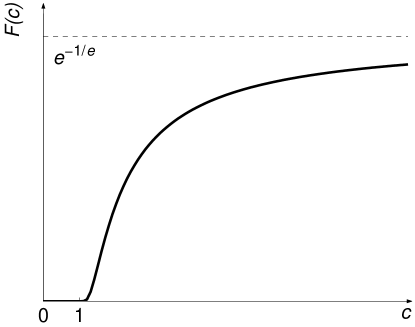
Figure 1: The phase transition of Theorem 3.2: in the subcritical phase $(0\leq c<1)$, the minimum probability of failure-free operation is zero; in the supercritical phase $(c>1)$, it is $\exp\left(-\frac{c}{e(c-1)}\right)$. Note that $F(c)$ approaches $e^{-1/e}$ as $c\to\infty$.

Remark 3.3

The proof of the theorem goes through [modulo obvious modifications involving the exponent in the $c>1$ case of (3.12)] if, instead of $\vartheta(x)$, we use any nonnegative function $f(x)$ that behaves like $1/x$ for large $x$.

Proof.

In order to carry on, we first need to gather some preliminary results. Once we have all the right pieces in place, the proof is actually surprisingly simple.

The first result we need is the following exact formula for $F_{\varepsilon}(G)$:

Lemma 3.4

For any acyclic digraph $G=(V,E)$ with $v(G)=n$, $F_{\varepsilon}(G)=(1-\varepsilon)^{n}$.

Proof.

Let $i_{1}<i_{2}<\ldots<i_{n}$ be an arrangement of the vertices of $G$ according to some linear extension [1] of the partial order $\preceq$ defined in Section 2.1. Then, for each $k\in[n]$,

$$i_{j}\not\succeq i_{k},\qquad 1\leq j<k,$$ (3.13)

so, by definition of $\varepsilon$-admissibility, we have for any $\mu\in{\mathcal{M}}^{G}_{\varepsilon}$

$$\mu\big{(}A_{i_{k+1}}|\bigcap\nolimits^{k}_{j=1}\overline{A_{i_{j}}}\big{)}\leq\varepsilon,\qquad 0\leq k\leq n-1.$$ (3.14)

Then

$$\mu\big{(}\bigcap_{i\in V}\overline{A_{i}}\big{)}=\big{(}1-\mu(A_{i_{1}})\big{)}\times\prod^{n-1}_{k=1}\left(1-\mu\big{(}A_{i_{k+1}}|\bigcap\nolimits^{k}_{j=1}\overline{A_{i_{j}}}\big{)}\right)\geq(1-\varepsilon)^{n}.$$ (3.15)

The choice $\mu=\pi^{V}_{\varepsilon}\equiv\prod_{i\in V}\nu^{i}_{\varepsilon}$ attains the bound in (3.15), and the lemma is proved. ∎

Next, we will need a result on the size of the largest reflexive, transitive closure of a vertex in the random acyclic digraph ${\mathbb{G}}_{d}(n,cn^{-1}\log n)$. Pittel and Tungol [37] showed that the following phase transition takes place as $c$ is varied:

Lemma 3.5

For the random acyclic digraph ${\mathbb{G}}_{d}(n,cn^{-1}\log n)$ one has the following:

1. If $c\geq 1$, then there exists a positive constant $A(c)$, such that

   $$\lim_{n\to\infty}{\mathbb{P}}\left\{\left|\gamma^{\star}_{n}-n\left(1-\frac{1}{c}\right)-\frac{2n\log\log n}{c\log n}\right|\leq\frac{A(c)n}{\log n}\right\}=1.$$ (3.16)

2. If $c<1$, then for every $\varkappa>0$,

   $$\lim_{n\to\infty}{\mathbb{P}}\left\{(1-\varkappa)n^{c}\log n<\gamma^{\star}_{n}\leq n^{c}\log n\right\}=1.$$ (3.17)

The exact (and rather unwieldy) expressions of Lemma 3.5 are more than is needed for the purposes of the present proof. We will settle for a rather more prosaic asymptotic form that follows directly from (3.16) and (3.17). Namely, whp

$$\gamma^{\star}_{n}(c)\sim\begin{cases}n^{c}\log n&\text{if $0\leq c<1$}\\ \\[-10.00002pt] \frac{2n\log\log n}{\log n}&\text{if $c=1$}\\ \\[-10.00002pt] n\left(1-\frac{1}{c}\right)&\text{if $c>1$}\end{cases},$$ (3.18)

where, as usual, the notation $a_{n}\sim b_{n}$ means that $a_{n}=b_{n}\big{(}1+o(1)\big{)}$.

Next, we need asymptotics of the function $\vartheta(x)$ for large $x$. To that end, we write

$$\lim_{x\to\infty}x\vartheta(x)=\lim_{x\to\infty}\left(1-\frac{1}{x+1}\right)^{x}=\frac{1}{e}.$$ (3.19)

In other words, $\vartheta(x)\sim\frac{1}{ex}$ as $x\to\infty$.

Finally, we will have use for the following two limits:

Lemma 3.6

$$\lim_{n\to\infty}\left(1-\frac{1}{n^{c}\log n}\right)^{n} = 0,\qquad 0\leq c<1$$ (3.20)

$$\lim_{n\to\infty}\left(1-\frac{\log n}{n\log\log n}\right)^{n} = 0.$$ (3.21)

Proof.

We will prove (3.20); the same strategy will work for (3.21) as well. Let us assume that $\log$ denotes natural logarithms [otherwise we can multiply the second term in parentheses of (3.20) by a suitable constant]. It suffices to show that

$$\lim_{n\to\infty}n\log\left(1-\frac{1}{n^{c}\log n}\right)=-\infty.$$ (3.22)

Using the inequality $\log x\leq x-1$, we have for each $n$

$$n\log\left(1-\frac{1}{n^{c}\log n}\right)\leq-\frac{n^{1-c}}{\log n}.$$ (3.23)

Given any $K>0$, one can find large enough $N$ such that the right-hand side of (3.23) is less than $-K$ for all $n\geq N$. Therefore the same holds for the left-hand side, and (3.22) is proved. ∎

The rest is fairly straightforward. Using Lemma 3.4 and (3.19), we get

$$F_{n}(c)=\big{(}1-\vartheta(\gamma^{\star}_{n}(c))\big{)}^{n}=\left(1-\frac{1+o(1)}{e\gamma^{\star}_{n}(c)}\right)^{n}.$$ (3.24)

Now, using the asymptotics in (3.18), we obtain that whp

$$F_{n}=\begin{cases}\big{(}1-\frac{1+o(1)}{n^{c}\log n}\big{)}^{n}&\text{if $c<1$}\\ \\[-10.00002pt] \big{(}1-\frac{1+o(1)}{2n\log\log n/\log n}\big{)}^{n}&\text{if $c=1$}\\ \\[-10.00002pt] \big{(}1-\frac{1+o(1)}{(1-c^{-1})n}\big{)}^{n}&\text{if $c>1$}\end{cases}.$$ (3.25)

Upon taking the limit as $n\to\infty$ of the expressions given in the right-hand side of (3.25) and using Lemma 3.6, we obtain (3.12), and the theorem is proved. ∎

3.3 Discussion

In retrospect, it is easy to see that Theorem 3.2 holds trivially under the independent failure model. In order to appreciate nontrivial features that appear once we pass to Pippenger’s model, we will invoke the game-theoretic interpretation given at the end of Section 2.2.

Consider a Programmer-Hacker game of the kind described in Section 2.2. Provided that the constant $\varepsilon_{0}$ picked by the Referee is sufficiently small, the Programmer has a good chance of winning if he sticks to the following strategy: Let $n_{0}$ be the smallest integer and $c$ the largest positive number, such that $\varepsilon_{0}\leq[e(1-1/c)n_{0}]^{-1}$ and $cn^{-1}_{0}\log n_{0}\leq 1$. The Programmer generates a random acyclic digraph ${\mathbb{G}}_{d}(n_{0},cn^{-1}_{0}\log n_{0})$ and uses it to construct a Boolean network ${\sf N}_{c}(n)$ by adding variable inputs, assigning gate labels, and designating the output gate, possibly in a completely arbitrary fashion. He then hands this network to the Hacker. (Note that both the Programmer and the Hacker have all the information needed to determine which function $f$ is computed by the network.) If $c$ is large enough, then Theorem 3.2 thus guarantees the existence of some $\delta<1/2$ such that, with probability $1-o(1)$, the network generated by the Programmer will $(\varepsilon_{0},\delta)$-compute $f$, regardless of the Hacker’s actions. More precisely, for any $\varkappa,\varkappa^{\prime}>0$, there exists large enough $N$ such that, for any $c\in(1,N/\log N)$ and for all $n\geq N$,

$${\mathbb{P}}\left(\begin{array}[]{c}\text{\small${\sf N}_{c}(n)$ $([e(1-1/c)n]^{-1},\delta)$-computes $f$}\\ \text{\small with $\left|(1-\delta)-\exp\left(-\frac{c}{e(c-1)}\right)\right|<\varkappa$}\end{array}\right)>1-\varkappa^{\prime}.$$ (3.26)

Provided that $e^{-c/[e(c-1)]}-\varkappa>1/2$ and $\varepsilon_{0}\leq[e(1-1/c)n_{0}]^{-1}$ for some $n_{0}\geq N$, the Programmer will win with probability at least $1-\varkappa^{\prime}$.

4 Pippenger’s model and stochastic domination

In Section 3.1 an argument based on the lopsided Lovász local lemma ([15], see also Theorem 3.1 in this paper) allowed us to pinpoint the possibility for a phase transition in Pippenger’s model on random graphs. In this section we show that the machinery of stochastic domination [26, 27, 28] enables us to carry out a more refined analysis of Pippenger’s model. [We hasten to note that many of the issues which we will touch upon have, in fact, already been discussed by Pippenger in Ref. [34], but without any systematic emphasis on stochastic domination.]

4.1 Stochastic domination: the basics

Once again, consider a finite acyclic digraph $G=(V,E)$ along with the measurable space $(\Omega,{\mathcal{F}})$, where $\Omega={\mathbb{B}}^{V}$ and ${\mathcal{F}}$ is the set of all subsets of $\Omega$. Elements of $\Omega$ are binary strings of length $v(G)$; we will denote the $i$th component (bit) of $\omega\in\Omega$ by $\omega(i)$. The total ordering of ${\mathbb{B}}$ induces the following partial order of $\Omega$:

$$\omega_{1}\prec\omega_{2}\quad\Longleftrightarrow\quad\omega_{1}(i)\leq\omega_{2}(i),\forall i\in V.$$ (4.1)

We say that a function $f:\Omega\to{\mathbb{R}}$ is increasing if $\omega_{1}\prec\omega_{2}$ implies $f(\omega_{1})\leq f(\omega_{2})$. An event $H\in{\mathcal{F}}$ is called increasing if its indicator function, ${\mathbf{1}}_{H}$, is increasing. Informally speaking, an event is increasing if its occurrence is unaffected by changing some bits from zero to one. Decreasing functions and events are defined in an obvious way. Given two probability measures $\mu,\nu$ on $(\Omega,{\mathcal{F}})$, we will say that $\mu$ is stochastically dominated by $\nu$ (and write $\mu\preceq_{s}\nu$) if, for every increasing function $f$, ${\mathbb{E}}_{\mu}(f)\leq{\mathbb{E}}_{\nu}(f)$. As usual, the expectation ${\mathbb{E}}_{\mu}(\cdot)$ is defined by

$${\mathbb{E}}_{\mu}(f):=\int_{\Omega}fd\mu\equiv\sum_{\omega\in\Omega}f(\omega)\mu(\omega).$$ (4.2)

Any probability measure $\mu$ on $(\Omega,{\mathcal{F}})$ is equivalent to a family $\{X_{i}:i\in V\}$ of ${\mathbb{B}}$-valued random variables via

$${\mathbb{P}}\big{(}\bigwedge_{i\in V}(X_{i}=\omega(i))\big{)}=\mu(\omega),\qquad\forall\omega\in\Omega$$ (4.3)

(also cf. Section 2.3). We will say that the $X_{i}$ have joint law $\mu$ if (4.3) holds. Then we have the following necessary and sufficient condition, due to Strassen [43], for one measure to dominate another (this is, in fact, a type of result that is proved most naturally by means of the so-called coupling method; see the monograph by Lindvall [28] for this as well as for many other useful applications of coupling).

Lemma 4.1

Let $\mu,\nu$ be probability measures on $(\Omega,{\mathcal{F}})$. Then $\mu\preceq_{s}\nu$ if and only if there exist families of random variables $\{X_{i}:i\in V\}$ and $\{Y_{i}:i\in V\}$, defined on a common probability space, with respective joint laws $\mu$ and $\nu$, such that $X_{i}\leq Y_{i}$ almost surely for each $i\in V$.

Next we need a sufficient condition for a given probability measure $\mu$ to dominate the Bernoulli product measure $\pi^{V}_{\eta}$. The following lemma is standard, and can be proved along the lines of Holley [23] and Preston [38]:

Lemma 4.2

Consider a family $\{X_{i}:i\in V\}$ of random variables with joint law $\mu$. Suppose that there exists a total ordering $<$ of $V$ such that, for any $i\in V$ and any two disjoint sets $Y,Y^{\prime}\subseteq V\backslash\{i\}$ with $j<i$ for all $j\in Y\cup Y^{\prime}$, we have

$${\mathbb{P}}_{\mu}\big{(}X_{i}=1|\bigwedge_{j\in Y}(X_{j}=1)\wedge\bigwedge_{j\in Y^{\prime}}(X_{j}=0)\big{)}\geq\eta,$$ (4.4)

whenever ${\mathbb{P}}_{\mu}\big{(}\bigwedge_{j\in Y}(X_{j}=1)\wedge\bigwedge_{j\in Y^{\prime}}(X_{j}=0)\big{)}>0$. Then $\mu\succeq_{s}\pi^{V}_{\eta}$.

Note that Lemma 4.2 can also go in the other direction: that is, if instead we write the $\leq$ sign in (4.4), then we will have $\mu\preceq_{s}\pi^{V}_{\eta}$.

Before we go on, let us introduce one more definition. Given $\eta\in(0,1)$, let us define a class ${\mathcal{W}}^{G}_{\eta}$ of probability measures on $(\Omega,{\mathcal{F}})$ as follows. Let $\{X_{i}:i\in V\}$ be the family of ${\mathbb{B}}$-valued random variables with joint law $\mu$. Then $\mu\in{\mathcal{W}}^{G}_{\eta}$ if, for any $i\in V$ and for any disjoint sets $Y,Y^{\prime}\subseteq V\backslash\bar{N}(i)$,

$$\mu\big{(}X_{i}=1|\bigwedge_{j\in Y}(X_{j}=1)\wedge\bigwedge_{j\in Y^{\prime}}(X_{j}=0)\big{)}\geq\eta,$$ (4.5)

whenever the event we condition on has positive probability.

4.2 Stochastic domination in Pippenger’s model

In this section we will use the machinery of stochastic domination to present a more delicate analysis of the $\varepsilon$-admissible model of Pippenger. Let us fix (yet another!) acyclic digraph $G=(V,E)$, which we will think of as a gate interconnection graph of a suitable class of Boolean networks equivalent modulo gate labels and the location of the output vertex (see Section 3.1 for details). Given a probability measure $\mu\in{\mathcal{M}}^{G}_{\varepsilon}$, let $\{X_{i}:i\in V\}$ be a family of ${\mathbb{B}}$-valued random variables with joint law $\mu$. Let us define $\tilde{X}_{i}:=1-X_{i}$ for each $i\in V$; clearly, $\tilde{X}_{i}$ is an indicator random variable for the event $\overline{A_{i}}\equiv\{\text{gate $i$ does not fail}\}$. Let $\eta:=1-\varepsilon$. The joint law $\tilde{\mu}$ of $\{\tilde{X}_{i}\}$ is such that, for any $i\in V$ and any two disjoint sets $Y,Y^{\prime}\in V\backslash\Gamma^{\star}(i)$,

$$\tilde{\mu}\big{(}\tilde{X}_{i}=1|\bigwedge_{j\in Y}(\tilde{X}_{j}=1)\wedge\bigwedge_{j\in Y^{\prime}}(\tilde{X}_{j}=0)\big{)}\geq\eta,$$ (4.6)

whenever the event we condition on has nonzero probability. Passing to the transitive closure graph $G^{\star}=(V,E^{\star})$, we can rewrite (4.6) as follows: for any $i\in V$ and any disjoint $Y,Y^{\prime}\subseteq V\backslash\bar{N}^{\star}(i)$,

$$\tilde{\mu}\big{(}\tilde{X}_{i}=1|\bigwedge_{j\in Y}(\tilde{X}_{j}=1)\wedge\bigwedge_{j\in Y^{\prime}}(\tilde{X}_{j}=0)\big{)}\geq\eta.$$ (4.7)

Comparing (4.7) and (4.5), we see that $\mu\in{\mathcal{M}}^{G}_{\varepsilon}$ implies $\tilde{\mu}\in{\mathcal{W}}^{G^{\star}}_{\eta}$.

Let us show now that, for any $\mu\in{\mathcal{M}}^{G}_{\varepsilon}$, the corresponding $\tilde{\mu}$ satisfies $\tilde{\mu}\succeq_{s}\pi^{V}_{\eta}$. We can use the same strategy as in the proof of Lemma 3.4. Namely, if we rearrange the vertices of $G$ according to some linear extension of the partial order $\preceq$, then $\tilde{\mu}$ is easily seen to satisfy the conditions of Lemma 4.2, and we obtain the claimed result. It follows directly from definitions that we have also $\mu\preceq_{s}\pi^{V}_{\varepsilon}$. We also point out that Strassen’s theorem [43] (Lemma 4.1 in this paper) can be used to give an amusing interpretation of Pippenger’s model in terms of an intelligent agent (“demon”) who, when faced with a realization of $\{X_{i}\}$ with joint law $\mu\in{\mathcal{M}}^{G}_{\varepsilon}$, can transform it into a realization of random variables i.i.d. according to $\pi^{V}_{\varepsilon}$ by changing some bits from 0 to 1, but none from 1 to 0. (The same observation has been first made by Pippenger [34], who substantiated it using a non-probabilistic result of Hwang [24].)

As part of our proof of Theorem 3.2, we have obtained the exact formula $F_{\varepsilon}(G)=(1-\varepsilon)^{v(G)}$ by arranging the vertices of $G$ according to a linear extension of the partial order $\preceq$. The same conclusion can be easily reached once we have established that, for any $\mu\in{\mathcal{M}}^{G}_{\varepsilon}$, we have $\mu\preceq_{s}\pi^{V}_{\varepsilon}$ [or, equivalently, that the corresponding $\tilde{\mu}\in{\mathcal{W}}^{G^{\star}}_{\eta}$ stochastically dominates $\pi^{V}_{\eta}$]; this extra information enables us to obtain many other useful estimates besides the one for $F_{\varepsilon}(G)$.

It is easy to see, for instance, that most of the “really interesting” events one would naturally associate with proper operation of the network (e.g., the event that the majority of the gates have not failed) are decreasing events. That is, if such an event occurs in a particular configuration $\omega$, then this event can be destroyed by introducing additional failed gates. The event that no gate fails is a particularly drastic example: it is destroyed if we change the status of even a single gate. Equivalently, we may pass to the corresponding probability measure $\tilde{\mu}$. In that case, given a configuration $\omega\in{\mathbb{B}}^{V}$, the gate failures will correspond to zero bits of $\omega$, with the nonzero bits indicating the gates that have not failed. Therefore we may consider increasing events if we agree to work with $\tilde{\mu}$ instead of $\mu$. Using the stochastic domination properties of $\tilde{\mu}$, we get that $\tilde{\mu}(H)\geq\pi^{V}_{\eta}(H)$ for any increasing event $H$.

As a simple example, consider the following set-up. Suppose we are given a network ${\sf N}$ whose output is the output of a gate that computes a Boolean function $\varphi:{\mathbb{B}}^{d}\to{\mathbb{B}}$. Suppose that the inputs to this gate come from the outputs of subnetworks ${\sf N}_{1},\ldots,{\sf N}_{d}$ (note that these subnetworks may, in general, share both gates and wires). Let $M$ be the event that the majority of the gates in ${\sf N}$ have not failed, let $M_{i}$, $1\leq i\leq d$, be the event that the majority of the gates in ${\sf N}_{i}$ have not failed, and let $L$ be the event that the output gate of ${\sf N}$ has not failed. Then $L\cap\bigcap^{d}_{i=1}M_{i}$ implies $M$, so that

$${\mathbb{P}}(M)\geq{\mathbb{P}}\big{(}L\cap\bigcap\nolimits^{d}_{i=1}M_{i}\big{)}={\mathbb{P}}\big{(}L|\bigcap\nolimits^{d}_{i=1}M_{i}\big{)}{\mathbb{P}}\big{(}\bigcap\nolimits^{d}_{i=1}M_{i}\big{)}.$$ (4.8)

Suppose that the underlying probability measure $\mu$ is $\varepsilon$-admissible. Then

$${\mathbb{P}}\big{(}L|\bigcap\nolimits^{d}_{i=1}M_{i}\big{)}\geq\eta.$$ (4.9)

Likewise by $\varepsilon$-admissibility, $\tilde{\mu}\succeq_{s}\pi^{\sf N}_{\eta}$ (see Section 2.2 for this notation). Therefore, since an intersection of increasing events is increasing, we have

$${\mathbb{P}}_{\tilde{\mu}}\big{(}\bigcap\nolimits^{d}_{i=1}M_{i}\big{)}\geq\pi^{\sf N}_{\eta}\big{(}\bigcap\nolimits^{d}_{i=1}M_{i}\big{)}.$$ (4.10)

The right-hand side of (4.10) can be bounded from below by means of the FKG inequality [18] (proved earlier by Harris [20] in the context of percolation) to give

$${\mathbb{P}}_{\tilde{\mu}}\big{(}\bigcap\nolimits^{d}_{i=1}M_{i}\big{)}\geq\prod^{d}_{i=1}\pi^{{\sf N}_{i}}_{\eta}(M_{i}).$$ (4.11)

Let $a$ be the number of gates in the smallest of the subnetworks ${\sf N}_{1},\ldots,{\sf N}_{d}$. Then, assuming that $\varepsilon\leq 1/2$, Azuma-Hoeffding inequality [4, 22] gives

$$\pi^{{\sf N}_{i}}_{\eta}(M_{i})\geq 1-e^{-a(4\eta-2)^{2}}.$$ (4.12)

Putting everything together, we get

$${\mathbb{P}}(M)\geq\eta\left(1-e^{-a(4\eta-2)^{2}}\right)^{d}.$$ (4.13)

This use of the FKG inequality is similar to that in Feder [34], whose work was concerned with the depth and reliability bounds for reliable computation of Boolean functions under the independent failure model.

At this point we also mention another PFM discussed by Pippenger in Ref. [34] — namely, the so-called $\varepsilon$-majorized model. Under this model, a network ${\sf N}$ is mapped to the set of all probability measures $\mu$ on ${\mathbb{B}}^{\hat{V}_{\sf N}}$ that are stochastically dominated by the Bernoulli product measure $\pi^{\sf N}_{\varepsilon}$. It follows easily from the discussion above that the $\varepsilon$-majorized model is more stringent than the $\varepsilon$-admissible model. As an example of its use, we can mention the work of Dobrushin and Ortyukov [12], where a result proven for the $\varepsilon$-majorized model automatically carries over to the $\varepsilon$-independent one.

5 Closing remarks and future directions

In this paper we have showed that a phase transition is possible in the $\varepsilon$-admissible PFM of Pippenger [34] as soon as random graphs show up in the picture. In doing so, we have barely scratched the surface of a wonderfully rich subject — namely, the statistical mechanics of multicomponent random systems on directed graphs. Most of the work connected to phase transitions in large combinatorial structures has been done in the context of undirected graphs, since the methods of statistical mechanics applicable to the study of combinatorial structures have been originally developed in that context as well.

For instance, the independent-set polynomial of a simple undirected graph [17, 21, 41] can also be viewed as a partition function of a repulsive lattice gas [42], and the powerful machinery of cluster expansions [10] developed in the latter setting can also be applied quite successfully to the former; the reader is encouraged to consult a recent paper by Scott and Sokal [39] for an exposition of these matters from the viewpoint of both statistical mechanics and graph theory. In the future we would like to study applications of statistical mechanics to combinatorial structures with directionality. So far, very few results along these lines have appeared; the papers of Whittle [45, 46] are among the few examples known to the present author where a partition function is constructed for a class of statistical-mechanical models on directed graphs. The relative dearth of applications of statistical mechanics to structures with directionality is due to the fact that, once directionality is introduced, the symmetry needed for the lattice-gas formalism is destroyed, and it is not immediately evident how one could relate combinatorial properties of directed graphs to mathematical objects of statistical mechanics. (Incidentally, this very point has also been brought up by Scott and Sokal [39].)

Appendix

Our goal in this appendix is to prove a theorem that can be thought of as a specialization of the lopsided Lovász local lemma of Erdős and Spencer [15] (see also Theorem 3.1) to families of random variables whose joint laws are elements of ${\mathcal{W}}^{G}_{\eta}$. Both the theorem and its proof go very much along the lines a similar result of Liggett, Schonmann, and Stacey [27], except that theirs was formulated for undirected graphs.

Theorem A.1

Let $G=(V,E)$ be a directed acyclic graph, in which every vertex has out-degree at most $\Delta\geq 1$. Let $\mu\in{\mathcal{W}}^{G}_{\eta}$ with $\varepsilon:=1-\eta\leq\Delta^{\Delta}/(\Delta+1)^{(\Delta+1)}$. Then $\mu\succeq_{s}\pi^{V}_{\rho}$, where

$$\rho=\left(1-\frac{\varepsilon^{1/(\Delta+1)}}{\Delta^{\Delta/(\Delta+1)}}\right)\left(1-(\varepsilon\Delta)^{1/(\Delta+1)}\right).$$ (A.1)

Proof.

First we need a lemma.

Lemma A.2

Let $G=(V,E)$ satisfy the conditions of Theorem A.1. Given $\eta\in(0,1)$, consider $\mu\in{\mathcal{W}}^{G}_{\eta}$. Suppose that there exist constants $\alpha,\lambda\in(0,1)$, such that

$$\varepsilon\leq(1-\alpha)(1-\lambda)^{\Delta},$$ (A.2)

$$\varepsilon\leq(1-\alpha)\alpha^{\Delta}.$$ (A.3)

Consider a family $\{X_{i}:i\in V\}$ of random variables with joint law $\mu$, and let $\{Y_{i}:i\in V\}$ be a family of random variables, independent of $\{X_{i}\}$ and with joint law $\pi^{V}_{\lambda}$. Let $Z_{i}:=X_{i}Y_{i}$ for each $i\in V$. Then, for each $i\in V$, each $Y\subseteq V\backslash\{i\}$, and each $z\in{\mathbb{B}}^{|Y|}$, we have

$${\mathbb{P}}\big{(}Z_{i}=1|\bigwedge\nolimits^{|Y|}_{j=1}(Z_{i_{j}}=z_{j})\big{)}\geq\alpha\lambda,$$ (A.4)

where the $i_{j}$ are elements of $Y$.

Remark A.3

The corresponding theorem of Liggett, Schonmann, and Stacey [27] is formulated in terms of an undirected graph $G$, with $\Delta$ being the maximum degree of a vertex. Therefore they need to impose an additional condition, namely that $i$ is adjacent to at most $\Delta-1$ vertices in $Y$. As a consequence, one has to make the replacement $\Delta\to\Delta-1$, e.g., in (A.1), (A.2) and (A.3). However, because here we deal with directed graphs and $\Delta$ is the maximum out-degree of a vertex, there are automatically no more than $\Delta$ vertices $j$ in $G$ with $(i,j)\in E$.

Proof.

Note that (A.4) is equivalent to

$${\mathbb{P}}\big{(}X_{i}=1|\bigwedge\nolimits^{|Y|}_{j=1}(Z_{i_{j}}=z_{j})\big{)}\geq\alpha$$ (A.5)

due to independence of $\{X_{i}\}$ and $\{Y_{i}\}$ and to the fact that $\lambda>0$. We will proceed by proving (A.5) by induction on $|Y|$.

Suppose first that $Y=\varnothing$. Then (A.5) is simply the statement that ${\mathbb{P}}(X_{i}=1)\geq\alpha$. Now, ${\mathbb{P}}(X_{i}=1)\geq\eta$ because $\mu\in{\mathcal{W}}^{G}_{\eta}$, and $\eta\geq\alpha$ by (A.3). Thus suppose that (A.5) holds for all $Y\subseteq V\backslash\{i\}$ with $|Y|<J$, where $J\geq 1$. We will prove that it also holds for $|Y|=J$.

Fix $Y=\{i_{1},\ldots,i_{J}\}$ and $z\in{\mathbb{B}}^{J}$. We write $Y$ as a disjoint union $M_{0}\cup M_{1}\cup M$, where

$$M_{0} := \{i_{j},1\leq j\leq J:\text{$(i,i_{j})\in E$ and $z_{j}=0$}\}$$ (A.6)

$$M_{1} := \{i_{j},1\leq j\leq J:\text{$(i,i_{j})\in E$ and $z_{j}=1$}\}$$ (A.7)

$$M := Y\backslash(M_{0}\cup M_{1}).$$ (A.8)

Let us also define the events

$$A_{0} := \{Z_{i_{j}}=0:i_{j}\in M_{0}\}$$ (A.9)

$$B_{0} := \{Y_{i_{j}}=0:i_{j}\in M_{0}\}$$ (A.10)

$$A_{1} := \{X_{i_{j}}=1:i_{j}\in M_{1}\}$$ (A.11)

$$A := \{Z_{i_{j}}=z_{j}:i_{j}\in N\}$$ (A.12)

Now, for any $j\in V$, $Z_{j}=1$ is by definition equivalent to both $X_{j}=1$ and $Y_{j}=1$. Furthermore, $\{X_{j}\}$ and $\{Y_{j}\}$ are independent. Therefore we can write

$${\mathbb{P}}\big{(}X_{i}=1|\bigwedge\nolimits^{J}_{j=1}(Z_{i_{j}}=z_{j})\big{)}={\mathbb{P}}\big{(}X_{i}=1|A_{0}\cap A_{1}\cap A\big{)}$$ (A.13)

Now

$${\mathbb{P}}\big{(}X_{i}=1|A_{0}\cap A_{1}\cap A\big{)} = 1-{\mathbb{P}}\big{(}X_{i}=0|A_{0}\cap A_{1}\cap A\big{)}$$ (A.14)

$$= 1-\frac{{\mathbb{P}}\big{(}X_{i}=0,A_{0}\cap A_{1}\cap A\big{)}}{{\mathbb{P}}\big{(}A_{0}\cap A_{1}\cap A\big{)}}$$

$$\geq 1-\frac{{\mathbb{P}}\big{(}X_{i}=0,A\big{)}}{{\mathbb{P}}\big{(}B_{0}\cap A_{1}\cap A\big{)}}$$

$$= 1-\frac{{\mathbb{P}}\big{(}X_{i}=0|A\big{)}}{{\mathbb{P}}\big{(}B_{0}\cap A_{1}|A\big{)}}.$$

Since $(i,i_{j})\not\in E$ for all $i_{j}\in M$, the numerator is at most $\varepsilon$. The denominator is equal to $(1-\lambda)^{|M_{0}|}{\mathbb{P}}\big{(}A_{1}|A\big{)}$. Assume that $M_{1}=\{k_{1},\ldots,k_{s}\}$, $s=|M_{1}|$. Then,

$${\mathbb{P}}\big{(}A_{1}|A\big{)} = {\mathbb{P}}\big{(}\bigwedge\nolimits^{s}_{\ell=1}(X_{k_{\ell}}=1)|A\big{)}$$ (A.15)

$$= {\mathbb{P}}\big{(}X_{k_{1}}=1|A\big{)}\prod^{s-1}_{\ell=1}{\mathbb{P}}\big{(}X_{k_{\ell+1}}=1|A,\bigwedge\nolimits^{\ell}_{m=1}(X_{k_{m}}=1)\big{)}$$

$$\geq \alpha^{|M_{1}|},$$

where in the last step we have applied the inductive hypothesis to each of the terms in the product. Therefore

$${\mathbb{P}}\big{(}X_{i}=1|A_{0}\cap A_{1}\cap A\big{)}\geq 1-\frac{\varepsilon}{(1-\lambda)^{|M_{0}|}\alpha^{|M_{1}|}}.$$ (A.16)

Since $|M_{0}|+|M_{1}|\leq\Delta$ by hypothesis, and $\varepsilon/(1-\alpha)\leq\alpha^{\Delta}\leq 1$ by (A.3), we have

$$(1-\lambda)^{|M_{0}|}\alpha^{|M_{1}|}\geq\left(\frac{\varepsilon}{1-\alpha}\right)^{(|M_{0}|+|M_{1}|)/\Delta}\geq\frac{\varepsilon}{1-\alpha}.$$ (A.17)

Therefore the right-hand side of (A.16) is at least $1-\varepsilon/[\varepsilon/(1-\alpha)]=\alpha$, and the lemma is proved. ∎

Now let $\{X_{i}\}$, $\{Y_{i}\}$, and $\{Z_{i}\}$ be as in Lemma A.2. Let $\nu$ be the joint law of $\{Z_{i}\}$. By construction, $Z_{i}\leq X_{i}Y_{i}$ for each $i\in V$, so $\mu\succeq_{s}\nu$ by Lemma 4.1. We now show that $\nu\succeq_{s}\pi^{V}_{\alpha\lambda}$. Let $<$ be an arbitrary total ordering of $V$. Then Lemma A.2 and Lemma 4.2 imply that $\nu\succeq_{s}\pi^{V}_{\alpha\lambda}$. Thus $\mu\succeq_{s}\pi^{V}_{\alpha\lambda}$.

To conclude the proof, suppose that

$$\varepsilon\leq\frac{\Delta^{\Delta}}{(\Delta+1)^{\Delta+1}}.$$ (A.18)

Let

$$\alpha=1-\frac{\varepsilon^{1/(\Delta+1)}}{\Delta^{\Delta/(\Delta+1)}}\quad\text{and}\quad\lambda=1-(\varepsilon\Delta)^{1/(\Delta+1)}.$$ (A.19)

Then $(1-\alpha)(1-\lambda)^{\Delta}=\varepsilon$, which yields (A.2). Condition (A.18) is equivalent to

$$\varepsilon^{1/(\Delta+1)}\leq\frac{\Delta^{\Delta/(\Delta+1)}}{\Delta+1},$$ (A.20)

which, when substitued into (A.19), yields

$$\alpha\geq 1-\frac{1}{\Delta+1}\quad\text{and}\quad\lambda\geq\frac{1}{\Delta+1}.$$ (A.21)

This shows that the choice we have made in (A.19) leads to $\alpha,\lambda\in[0,1]$, and that $1-\lambda\geq\alpha$. The latter inequality implies (A.3). Therefore, by Lemma A.2, $\mu\succeq_{s}\pi^{V}_{\alpha\lambda}$, and the theorem is proved. ∎

It is important to mention that Theorem A.1 is useful only when $G$ is not transitively closed, i.e., when $(i,j)\in E$ and $(j,k)\in E$ does not imply $(i,k)\in E$. Otherwise one can partially order the vertices of $G$ by defining $i\preccurlyeq j$ if $(i,j)\in E$ for distinct $i,j\in V$, and $i\preccurlyeq i$ for each $i\in V$. As usual, let $i_{1}<\ldots<i_{v(G)}$ be a total order of $V$ according to some linear extension of $\preccurlyeq$. Thus, for any $i_{j}$, all the $i_{k}$ with $i_{k}<i_{j}$ and distinct from $i_{j}$ are not in $\bar{N}(i_{j})$. Therefore we can apply Lemma 4.2 directly to any $\mu\in{\mathcal{W}}^{G}_{\eta}$ to conclude that $\mu\succeq_{s}\pi^{V}_{\eta}$. This is, in fact, precisely the case we have dealt with in this paper — namely, when $G$ is a transitive closure of some other acyclic digraph $G_{0}$.

References

- [1] M. Aigner, Combinatorial Theory, Springer-Verlag, Berlin, 1979.
- [2] R. Albert and A.-L. Barabási, Statistical mechanics of complex networks, Rev. Mod. Phys. 74 (2002), 47–97.
- [3] N. Alon and J.H. Spencer, The Probabilistic Method, 2nd ed., Wiley, New York, 2000.
- [4] K. Azuma, Weighted sums of certain dependent variables, Tôhoku Math. J. 3 (1967), pp. 357–367.
- [5] A. Barak and P. Erdős, On the maximal number of strongly independent vertices in a random acyclic directed graph, SIAM J. Algebraic and Discrete Methods 5 (1984), 508–514.
- [6] G. Biroli, R. Monasson, and M. Weigt, A variational description of the ground state structure in random satisfiability problems, Eur. Phys. J. B 14 (2000), 551–568.
- [7] B. Bollobás, Random Graphs, 2nd ed., Cambridge University Press, Cambridge, 2001.
- [8] B. Bollobás, C. Borgs, J.T. Chayes, J.H. Kim, and D.B. Wilson, The scaling window of the 2-SAT transition, Random Struct. Alg. 18 (2001), 201–256.
- [9] C. Borgs, J.T. Chayes, and B. Pittel, Phase transition and finite-size scaling for the integer partitioning problem, Random Struct. Alg. 19 (2001), 247–288.
- [10] R.L. Dobrushin, Estimates of semi-invariants for the Ising model at low temperatures, Topics in Statistical and Theoretical Physics, American Mathematical Society Translations, Ser. 2, vol. 177 (1996), 59–81.
- [11] R.L. Dobrushin and S.I. Ortyukov, Lower bound for the redundancy of self-correcting arrangements of unreliable functional elements, Prob. Inf. Transm. 13 (1977), 59–65.
- [12] R.L. Dobrushin and S.I. Ortyukov, Upper bound on the redundancy of self-correcting arrangements of unreliable functional elements, Prob. Inf. Transm. 13 (1977), 203–218.
- [13] R. Durrett, Probability: Theory and Examples, 2nd ed., Wadsworth, Belmont, 1996.
- [14] P. Erdős and L. Lovász, Problems and results on 3-chromatic hypergraphs and some related questions, Infinite and Finite Sets, A. Hajnal et al., eds., North-Holland (1975), 609–628.
- [15] P. Erdős and J. Spencer, Lopsided Lovász local lemma and Latin transversals, Discrete Appl. Math. 30 (1991), 151–154.
- [16] T. Feder, Reliable computation by networks in the presence of noise, IEEE Trans. Inform. Theory 35 (1989), 569–571.
- [17] D.C. Fisher and A.E. Solow, Dependence polynomials, Discrete Math. 82 (1990), 251–258.
- [18] C.M. Fortuin, P.W. Kasteleyn, and J Ginibre, Correlation inequalities on some partially ordered sets, Commun. Math. Phys. 22 (1971), 89–103.
- [19] P. Gács and A. Gál, Lower bounds for the complexity of reliable Boolean circuits with noisy gates, IEEE Trans. Inform. Theory 40 (1994), 579–583.
- [20] T.E. Harris, A lower bound on the critical probability in a certain percolation process, Proc. Cambridge Phil. Soc. 56 (1960), 13–20.
- [21] C. Hoede and X.-L. Li, Clique polynomials and independent set polynomials of graphs, Discrete Math. 125 (1994), 219–228.
- [22] W. Hoeffding, Probability inequalities for sums of bounded random variables, J. Amer. Stat. Assoc. 58 (1963), 13–30.
- [23] R. Holley, Remarks on the FKG inequalities, Commun. Math. Phys. 36 (1974), 227–231.
- [24] F.K. Hwang, Majorization on a partially ordered set, Proc. Amer. Math. Soc. 76 (1979), 199–203.
- [25] S. Janson, T. Łuczak, and A. Ruciński, Random Graphs, Wiley, New York, 2000.
- [26] T.M. Liggett, Interacting Particle Systems, Springer, New York, 1985.
- [27] T.M. Liggett, R.H. Schonmann, and A.M. Stacey, Domination by product measures, Ann. Probab. 25 (1997), 71–95.
- [28] T. Lindvall, Lectures on the Coupling Method, Wiley, New York, 1992.
- [29] B. Luque and R.V. Solé, Phase transitions in random networks: simple analytic determination of critical points, Phys. Rev. E 55 (1997), 257–260.
- [30] O.C. Martin, R. Monasson, and R. Zecchina, Statistical mechanics methods and phase transitions in optimization problems, Theoret. Comput. Sci. 265 (2001), 3–67.
- [31] D.E. Muller, Complexity in electronic switching circuits, IRE Trans. Electr. Comput. 5 (1956), 15–19.
- [32] J. von Neumann, Probabilistic logics and the synthesis of reliable organisms from unreliable components, Automata Studies, C.E. Shannon and J. McCarthy, eds., Princeton University Press (1956), 329–378.
- [33] N. Pippenger, Reliable computation by formulas in the presence of noise, IEEE Trans. Inform. Theory 34 (1988), 194–197.
- [34] N. Pippenger, Invariance of complexity measures for networks with unreliable gates, J. Assoc. Comput. Machinery 36 (1989), 531–539.
- [35] N. Pippenger, Developments in “The Synthesis of Reliable Organisms from Unreliable Components,” Legacy of J. von Neumann, Proceedings of Symposia in Pure Mathematics, vol. 50 (1990), 311–324.
- [36] N. Pippenger, G.D. Stamoulis, and J.N. Tsitsiklis, On a lower bound for the redundancy of reliable networks with noisy gates, IEEE Trans. Inform. Theory 37 (1991), 639–643.
- [37] B. Pittel and R. Tungol, A phase transition phenomenon in a random directed acyclic graph, Random Struct. Alg. 13 (2001), 164–184.
- [38] C.J Prestion, A generalization of the FKG inequalities, Commun. Math. Phys. 36 (1974), 233–242.
- [39] A.D. Scott and A.D. Sokal, The repulsive lattice gas, the independent-set polynomial, and the Lovász local lemma, cond-mat/0309352 at arXiv.org.
- [40] G. Semerjian and L.F. Cugliandolo, Cluster expansions in dilute systems: applications to satisfiability problems and spin glasses, Phys. Rev. E 64 (2001), 036115.
- [41] J.B. Shearer, On a problem of Spencer, Combinatorica 5 (1985), 241–245.
- [42] B. Simon, The Statistical Mechanics of Lattice Gases, Princeton University Press, Princeton, 1993.
- [43] V. Strassen, The existence of probability measures with given marginals, Ann. Math. Statist. 36 (1965), 423–439.
- [44] I. Wegener, The Complexity of Boolean Functions, Wiley, New York, 1987.
- [45] P. Whittle, The statistics of random directed graphs, J. Stat. Phys. 56 (1989), 499–516.
- [46] P. Whittle, Fields and flows on random graphs, Disorder in physical systems, G.R. Grimmett and D.J.A. Welsh, eds., Oxford University Press (1990), 337–348.