Generic $3$-connected planar constraint systems are not soluble by radicals

Abstract.

We show that planar embeddable $3$-connected CAD graphs are generically non-soluble. A CAD graph represents a configuration of points on the Euclidean plane with just enough distance dimensions between them to ensure rigidity. Formally, a CAD graph is a maximally independent graph, that is, one that satisfies the vertex-edge count $2v-3=e$ together with a corresponding inequality for each subgraph. The following main theorem of the paper resolves a conjecture of Owen [11] in the planar case. Let $G$ be a maximally independent $3$-connected planar graph, with more than 3 vertices, together with a realisable assignment of generic dimensions for the edges which includes a normalised unit length (base) edge. Then, for any solution configuration for these dimensions on a plane, with the base edge vertices placed at rational points, not all coordinates of the vertices lie in a radical extension of the dimension field.

1. Introduction

A fundamental problem in Computer Aided Design (CAD) is the formulation of effective algebraic algorithms or numerical approximation schemes which solve for the location of points on a plane, given a set of relative distances between them. The relative distances are usually called dimensions in CAD by analogy with the dimensions on a dimensioned drawing and we will adopt that terminology here. For CAD applications the relevant class of configurations are those for which the dimensions are just sufficient to ensure that the points are located rigidly with respect to one another. It is a well known result of Laman [9] that the graphs underlying generically rigid configurations (frameworks) have a simple combinatorial description. In our terminology they are the so-called maximally independent graphs, that is, those satisfying the vertex-edge count $2v-3=e$ together with a corresponding inequality for each subgraph.

A number of algebraic and numerical methods have been proposed for solving these plane configurations (Owen [11], Bouma et al [2], Light and Gossard [10]) and these have been successfully implemented in CAD programs. Algebraic and combinatorial algorithms for graphs are particularly desirable for their speed and robustness and the resulting dramatic efficiency gains. For instances of this see, for example, the quadratic extension algorithm of [11], the graph decomposition algorithm of Hopcroft and Tarjan [8], or the combinatorial approach to protein molecule flexibility in Jacobs et al [5].

Current algebraic methods for solving CAD graphs assemble the solution for complete configurations from the solutions of rigid subcomponents and the assembly process involves only rigid body transformations, fusion at vertex pairs, and the solution of quadratic equations. The simplest subcomponent is a triangle of points which is solvable by quadratic equations and it thus follows that if the original configuration is assembled from triangles then it is solvable through successive quadratic extensions of the ground dimension field. The other subcomponents possible in this process are all represented by graphs which are $3$-connected (in the usual sense of vertex $3$-connected [14]) and so the problem of solving general configurations passes to the problem of solving configurations which are represented by $3$-connected graphs. Determination of $3$-connectivity can be effected rapidly with order $O(v+e)$. (See [8].)

We have previously suggested that with generic dimension values a subcomponent which is represented by a $3$-connected graph cannot be solved by quadratic equations (Owen [11]). Configurations that can be solved in this way are also known as ”ruler and compass constructible” and Gao and Chou [6] have given a procedure for determining in principle if any given configuration is ruler and compass constructible. However their analysis is based on the detail of derived elimination equations and they do not address the problem of generic solubility or non-solubility for general classes of graphs.

Despite the importance of algebraic solubility, the intractability or otherwise of generic $3$-connected configurations has not been put on a firm theoretical basis and in the present paper we begin such a project.

The solution configurations that we consider are comprised of points in the plane with a number of specified distances (dimensions) between them. With the natural correspondence of points to vertices and constraint pairs to edges each constraint system has an associated abstract graph. It is the nature of the abstract graph that is significant for the solubility of the constraint system and we shall be concerned with the situation where the abstract graph is a planar graph in the usual graph-theoretic sense; it can be drawn with edges realised by curves in the plane with no crossings.

We show that a planar $3$-connected maximally independent graph with generic dimensions is not only not solvable by quadratic extensions but is not soluble by radical extensions, that is, by means of the extraction of roots of arbitrary order together with the basic arithmetical operations. In fact our methods make use of some intricate planar graph theory leading to a edge contraction reduction scheme which is also of independent interest. The main theorem of the paper can be stated as follows.

Theorem 1.1.

Let $G$ be a maximally independent $3$-connected planar graph, with more than 3 vertices, together with a realisable assignment of generic dimensions for the edges which includes a normalised unit length (base) edge. Then, for any solution configuration for these dimensions on a plane, with the base edge vertices placed at rational points, not all coordinates of the vertices lie in a radical extension of the dimension field.

It follows in particular that the current algebraic schemes already solve all of the generic configurations with a planar graph that can be solved by radical extensions ! Also, we conjecture that planarity is not necessary for this conclusion.

Recall that a celebrated and fundamental achievement of classical Galois theory is that a polynomial of degree 5 or more, with rational coefficients, is not generally soluble by radical extensions over ${\mathbb{Q}}$. For a generic version of this, one can assert that a generic monic polynomial of degree $r\geq 5$ is not soluble by radical extensions of the base field ${\mathbb{Q}}(\{d\})$, where $\{d\}=\{d_{1},...,d_{r-1}\}$ are the generic (algebraically independent) coefficients. In this case, with coefficient field understood, the polynomial is said to be, simply, non-soluble. These facts suggest that if one is presented, as we are here, with $N$ polynomial equations in $N$ unknowns, with no apparent step by step solution scheme involving at most degree 4 polynomials, then solutions will not lie in radical extensions of the coefficient field. On the other hand, possibly working against this intuition is the fact that our constraint equations are all of quadratic type, in four variables, with a single generic constant term, and the variables of the equations reflect a (planar) graph structure which may possess an intrinsic reduction scheme. However our result shows that in fact there can be no grounds for a solution scheme by radical extraction which embraces more than the known quadratically soluble graphs. To paraphrase Theorem 1.1, planar embeddable $3$-connected CAD graphs are generically non-soluble.

Let us now outline the structure of the proof, the entirety of which is lengthy and eclectic, making use of graph theory, elimination theory for the ideals of complex affine varieties, Galois theory for specialised coefficient fields, and a brute force demonstration of the non-solubility of a vertex minimal $3$-connected maximally independent planar graph. We refer to this graph, indicated in Figure 1, as the doublet.

Figure 1. The Doublet and $K_{33}$.

The fact that the generic doublet graph is not soluble by radicals is obtained in Section 8 by first obtaining an explicit integral dimensioned doublet which is not soluble. Here the Galois groups of univariate polynomials in the elimination ideals for the constraint equations are computed with some computer algebra assistence. Generic non-solubility then follows from our Galois group specialisation theorem.

The strategy of the proof is to show that if there exists a graph $G$ which is maximally independent, planar, 3-connected and radically soluble then there is a smaller such graph with fewer vertices. By the minimality of the doublet this implies that the doublet is radically soluble which gives the desired contradiction

There are two aspects to the reduction step. The first of these is purely graph theoretic and is dealt with in the extensive analysis of Section 4. The main theorem there shows that a 3-connected planar maximally independent graph $G$ has either an edge $e$ in a triangle of edges which can be contracted to give a smaller such graph $G/e$, or has a rigid subgraph which can be replaced by a triangle to produce a smaller such graph, $H$ say. The second aspect is to connect the solubility of the (finite) variety of solutions for the dimensioned graph $G$ to that of the varieties of the resulting smaller dimensioned graphs. In the latter case we can simply compare generic constraint equations (see Proposition 8.1) to deduce that

$$\mbox{generic }G\mbox{ radical }\Rightarrow\mbox{generic }H\mbox{ radical }$$

However the former case of edge contraction is much more subtle. We approach this by noting first that the complex variety $V(G/e)$ of solutions for the generic contracted graph is identifiable with the variety of solutions for $G$ with partially specialised dimensions, with the contracted edge dimension $d_{e}$ specialised to $0$ and the two other edges of the contracted triangle specified as being equal. This gives the easy implication

$$\mbox{specialised }G\mbox{ radical }\Rightarrow\mbox{generic }G/e\mbox{ radical }$$

However we now need the final step, that is the implication

$$\mbox{generic }G\mbox{ radical }\Rightarrow\mbox{specialised }G\mbox{ radical }$$

To obtain this we consider carefully the polynomials which are the generators of the single variable elimination ideals associated with the constraint equations. We relate these generators to the corresponding polynomials for the ideals of the specialised equations. In fact we relate the solubility of these polynomials through a two-step process for the double specialisation. This is effected in Sections 5, 6. The proof of the final step is then completed by means of another application of the Galois group specialisation theorem, Theorem 7.2. This theorem asserts, roughly speaking, that the Galois group of a polynomial $p$ is a subgroup of the Galois group of a polynomial $P$ when $p$ derives from $P$ by partial specialisation of coefficients. We were unable to find a reference for this seemingly classical assertion.

Let us highlight two very important ideas which run through the proof of the reduction step for edge contractions (Theorem 6.1).

The first of these is that we must restrict attention to graphs whose constraint equations, both generic and specialised, have finitely many complex solutions. This form of rigidity for complex variables we call zero dimensionality and its significance is explained fully in the next section. It guarantees that univariate elimination ideals for the constraint equations are generated by univariate polynomials. Unfortunately, to maintain zero dimensionality our contraction scheme to the doublet must operate entirely in the framework of maximally independent graphs and it is this that necessitates the extended graph theory of Section 4.

The second important idea is that the constraint equations happen to be of parametric type. As is well known this means that various associated complex affine varieties are irreducible and in particular (Theorem 2.8) this is so for the so-called big variety in which the coordinates of vertices and the dimensions of edges are viewed as complex variables. With irreducibility present we can arrange the univariate generators of single variable elimination ideals to be irreducible over the appropriate field (Theorem 5.2) and so either all roots of the generator are radical or none are. Now it is the case that not every root of the generator need derive from a solution of the constraint equations. Thus the fact that either all roots or no roots are radical allows us to compare the solubility or otherwise of $G$ and $G/e$ by examining the solubility or otherwise of these univariate generators (Theorem 5.3).

Finally, we remark that the assumption that graphs have a planar embedding is used to guarantee that there is a reduction scheme to a minimal graph based on contracting edges. We expect that there are more general reduction schemes which terminate in either the doublet or the non-planar graph $K_{33}$. Also we are able to show that $K_{33}$ is generically non-soluble and this gives further support to our conjecture that general $3$-connected maximally independent graphs are non-soluble.

The results of this article were announced at the Fourth International Workshop on Automated Deduction in Geometry in September 2002 [12]. We thank Walter Whiteley for helpful discussions and for directing our attention to the paper of Asimov and Roth [1]

2. Constraint equations and algebraic varieties

We begin by formulating the main problem which is to determine the complex algebraic variety arising from the solutions to the constraint equations of a normalised dimensioned graph.

Let $G=(V,E)$ be a graph with vertex set $V$ and edge set $E$. We are concerned with the problem of determining coordinates $(x_{v},y_{v})$ for each vertex $v$ so that for some preassigned dimensions for the edges $e$ in $E$, we have solutions to the set of equations

$$f_{e}=0,~{}~{}~{}~{}~{}~{}e\in E,$$

where, for the edge $e=(vw)$,

$$f_{e}=(x_{v}-x_{w})^{2}+(y_{v}-y_{w})^{2}-d_{e}.$$

The dimensions $d_{e}$ are taken to be nonnegative real numbers, representing the square of the edge lengths of realised graphs.

It is convenient to refer to the set $\{f_{e}\}$ as a set of (unnormalised) constraint equations for the graph. Although in practice one is interested primarily in the real solutions in $\mathbb{R}^{2}$ for the vertices, which in turn account for the Euclidean realisations of the dimensioned graph, it is essential to our approach that we consider all complex solutions. In this case solutions always exist and we can employ the elimination theory for complex algebraic varieties.

Bearing in mind the multiplicity of solutions associated with Euclidean isometries we assume that for some base edge $b=(vw)$ in $E$ we have $d_{b}=1$ and the specification $(x_{v},y_{v})=(0,0),(x_{w},y_{w})=(1,0).$ This gives rise to a set of normalised constraint equations $\{f_{e}\}$. If, in addition, the dimensions are algebraically independent then we say that $\{f_{e}\}$ is a set of generic constraint equations for $G$. We shall generally assume that dimension sets and sets of constraint equations are normalised.

Let $(G,\{d_{e}\})$ be a normalised dimensioned graph with $n$ vertices and let $x_{i},y_{i},1\leq i\leq n-2$, be the coordinate variables for the non-base vertices. We write $V(\{f_{e}\})$ for the complex affine variety in $\mathbb{C}^{2n-4}$ determined by the corresponding set of constraint equations $\{f_{e}\}$.

We now give some definitions which give precise meanings to the terms generic and rigid. There is a close connection between our formalism and that of the theory of rigid frameworks (see Whiteley [16] and Asimow and Roth [1]) and in particular the notion of an independent graph is taken from this context.

Definition 2.1.

The dimensioned graph $(G,\{d_{e}\})$ is said to be zero dimensional if the complex algebraic variety $V(\{f_{e}\})$ is zero dimensional, that is, $V(\{f_{e}\})$ is a finite non-empty set.

Definition 2.2.

Let $G$ be a graph with $v_{G}$ vertices and $e_{G}$ edges. Then $G$ is said to be independent if for every vertex induced subgraph $H$, we have $2v_{H}-e_{H}\geq 3$. The graph $G$ is said to be maximally independent if it is independent and in addition $2v_{G}-e_{G}=3$.

The graphs for which generic dimensions give zero dimensional varieties admit a simple combinatorial description as we see below. These maximally independent graphs are also known colloquially as CAD graphs. This equivalence follows from our variant of Laman’s theorem. In fact we shall only need one direction, proved in Theorem 2.4 namely that maximally independent graphs with generic dimensions are zero dimensional.

Let us indicate more fully the nature and significance of zero dimensionality.

Zero dimensionality for dimensioned graphs might also be termed complex rigidity. For non-generic dimensions it is a stronger requirement than the rigidity of the graph as a bar-joint structure as given in [1] and [16]. To appreciate this consider the maximally independent graph in Figure 2 which we view as a generically dimensioned graph with normalised dimensions $\{d_{e}\}$. The two arrowed edges suggest a specialisation of $\{d_{e}\}$ to a new dimension set for the same graph in which the arrowed edges have length zero and two pairs of edges are of equal length. Despite the fact that the resulting semi-generic bar-joint structure is physically rigid and that the original graph has been contracted onto a maximally independent graph (the doublet), the specialised dimensioned graph is not zero-dimensional. In this case the variety $V^{\prime}$ is a one-dimensional variety in $\mathbb{C}^{12}$ which meets the real subset $\mathbb{R}^{12}$ in a finite set.

The graph in Figure 2 is not $3$-connected. In fact it is quadratically soluble in the sense expressed in Theorem 3.2. However the doublet is $3$-connected and, as we will show in a subsequent section, it is not quadratically soluble. This observation indicates that in any reduction scheme for the proof involving edge contractions it is necessary to work within the category of zero dimensional graphs rather than rigid graphs in the usual sense.

Figure 2. Specialisation of a quadratically soluble graph onto a doublet.

.

The following general theorem will be used in the proof of Theorem 2.4. By a specialisation of the dimension set $\{d_{e}\}$ in $\mathbb{C}^{n}$ (generally an algebraically independent set) we mean a set $\{d_{e}^{\prime}\}$ in which some or all of the $d_{e}$ have been replaced by rational numbers.

Theorem 2.3.

Let $V$ be a complex affine variety in $\mathbb{C}^{n}$ defined by polynomial equations of the form

$$f_{i}=h_{i}(\{x_{j}\})-d_{i}=0,~{}~{}~{}~{}1\leq i\leq n,$$

where $\{h_{i}\}$ are polynomials with rational coefficients in the complex variables $\{x_{j}\}=\{x_{1},...,x_{n}\}$, and where $\{d_{i}\}$ a set of constants in $\mathbb{C}$. If $J$ is the $n\times n$ matrix $J=(J_{ij})=(df_{i}/dx_{j})$ and $\det(J)$ is not identically zero as a polynomial in $\{x_{j}\}$ then

(1) The coordinates $\{x_{j}\}$ of any zero of $V$ are algebraically independent as a set if and only if the constants $\{d_{i}\}$ are algebraically independent as a set.

(2) If $\{d_{i}\}$ are algebraically independent then $\dim(V)=0$.

Proof.

Suppose that $\{d_{i}\}$ are algebraically dependent then there is some polynomial $p$ in $n$ variables with $p(d_{1},\dots,d_{n})=0.$ Define the polynomial $q$ by $q(\{x_{j}\})=p(h_{1}(\{x_{j}\}),\dots,h_{n}(\{x_{j}\}))$. Then $q$ is not the zero polynomial because $\det(dh_{i}/dx_{j})$ is not zero and so $q$ has a point where it evaluates non-zero. On the other hand it is clear that $q$ vanishes at any zero of $V$.

Conversely, suppose that $\{x_{j}\}$ are algebraically dependent. Then there is some polynomial $q$ in $n$ variables with $q(\{x_{j}\})=0$. Consider ideal $I=\langle f(\{d_{i}\},\{x_{j}\}),q(\{x_{j}\})\rangle$ and its variety $W$ in $\mathbb{C}^{2n}$ (where we abuse notation with $d_{1},\dots,d_{n}$ variables). This variety has dimension $n-1$ because it is isomorphic to $V(\langle q(\{x_{j}\})\rangle)$ in $\mathbb{C}^{n}$ under the isomorphism $(\{d_{i}\},\{x_{j}\})\to\{x_{j}\}$. On the other hand if the elimination ideal $I\cap\mathbb{C}[\{d_{i}\}]$ is empty then it follows from the closure theorem (see Theorem 5.1) that $W$ has dimension at least $n$. This proves the existence of a non zero polynomial $p(\{d_{i}\})$ in $I$. This polynomial evaluates to zero on the specific dimensions associated with the point $\{x_{j}\}$ since the generators of $I$ vanish on these points.

Any algebraically independent set $\{x_{j}\}$ defines an algebraically independent set $\{d_{i}\}$ for which $V$ is not empty. It follows that $V$ is not empty for all algebraically independent $\{d_{i}\}$ because $V$ is empty only if the ideal of $V$ contains a constant element of the field $\mathbb{Q}(\{d_{i}\})$. Also, any zero of $V$ for algebraically independent $\{d_{i}\}$ has algebraically independent coordinates $\{x_{j}\}$ and so every point of $V$ has  det$(J)$ non-zero. It follows that  dim$(V)=0.$

∎

The next theorem is our variant of Laman’s theorem.

Theorem 2.4.

Let $G$ be a maximally independent graph with $e$ edges and normalised constraint equations $\{f_{i}\}$, and let $V$ be the associated variety in $\mathbb{C}^{e-1}$ for algebracialy independent $\{d\}$. Then   dim$(V)=0$.

Proof.

The normalised constraint equations have the form required by Theorem 2.3 above while Theorem 6.5 of [9] implies that $\det(J)$ is not zero as a polynomial in $\{x_{j}\}$. ∎

We shall use elimination theory to study the varieties arising from various ideals generated by the constraint equations. In order to keep track of the nature of solutions (whether they are radical or not) it will be important, as we have intimated in the introduction, to identify generators of one variable elimination ideals which are irreducible polynomials. Theorem 2.8 below will be needed to achieve this.

Definition 2.5.

Let $I$ be an ideal in the polynomial ring $k[x_{1},...,x_{m}]$ over a field $k$ of characteristic zero. Then $I$ is prime if whenever $fg$ is in $I$ then either $f$ is in $I$ or $g$ is in $I$.

Proposition 2.6.

If $I$ is a prime ideal in $k[x_{1},...,x_{m}]$ and if $\{x_{i_{1}},...,x_{i_{t}}\}$ is a subset of $\{x_{i}\}$ then the elimination ideal

$$I\cap k[x_{i_{1}},...,x_{i_{t}}]$$

is also a prime ideal.

We now make a simple but important observation. The constraint equations for a graph are a parametric set when viewed as equations in the vertex coordinate variables and the dimensions. Indeed they are parametric in the vertex coordinate variables. From this it follows that various associated complex algebraic varieties are irreducible. For a discussion of such irreducibility see [4]. Thus we have the following general theorem which in turn gives the irreducibility of what we call the big variety $V_{b}$.

Theorem 2.7.

Let $x=\{x_{1},\dots,x_{m}\},d=\{d_{1},\dots,d_{r}\}$ be indeterminates defining the polynomial ring $\mathbb{Q}[x,d]$. Let $f_{i}(x,d)$ be polynomials of the form $h_{i}(x)-d_{i},1\leq i\leq r$, and let $I$ be the ideal of polynomials in $\mathbb{Q}[x,d]$ which vanish on the variety determined by $\{f_{i}:1\leq i\leq r\}$. Then $I$ is a prime ideal.

Theorem 2.8.

Let $G$ be a maximally independent graph with $n$ vertices and let $\{f\}$ be the normalised constraint equations for $G$ for the dimension set $\{d_{e}\}=\{d_{1},...,d_{r}\}$ (where $r=|E(G)|-1$). Let $V_{b}\subseteq\mathbb{C}^{2n-4+r}$ be the complex affine variety determined by $\{f\}$ as polynomial functions belonging to

$${\mathbb{Q}}[d_{1},...,d_{r},x_{1},...,x_{n-2},y_{1},...,y_{n-2}].$$

Then $V_{b}$ is irreducible.

3. Connectedness and quadratic solvability

The most tractable CAD graphs from the perspective of solvability are those which can be reduced to a collection of triangle graphs by successive disconnections at vertex pairs. In this section we indicate the way in which these graphs are quadratically soluble. We also recall various notions of connectivity for graphs.

Definition 3.1.

Let $G$ be a maximally independent graph and let $V$ be the variety defined by the constraint equations with generic normalised dimensions $\{d_{e}\}$.

(i) $G$ is said to be (generically) quadratically soluble (or simply QS) if every coordinate of every point of $V$ lies in an extension of the base field $\mathbb{Q}(\{d_{e}\})$ of degree $2^{n}$ for some $n$.

(ii) $G$ is said to be soluble by radicals (or RS), or, simply, soluble, if every such coordinate lies in a radical extension of the base field.

One could equally well define what it means for a specific dimensioned graph to be QS or RS. For example it would be of interest to know if particular graphs with integral dimensions are soluble. Such problems lead rapidly into arithmetical problems associated with multi-variable diophantine analysis and, with the exception of some considerations of integral doublets, we shall not address such non-generic issues.

The field $\mathbb{Q}(\{d_{e}\})$ is the field of fractions of polynomials in the dimensions. An irreducible quadratic polynomial over this base field determines a field extension of degree 2 and so a sequence of $n$ irreducible quadratic polynomials, with coefficients in the new fields, give rise to a final field extension of degree $2^{n}$. Moreover any field extension of this degree arises in this way. It follows that if a maximally independent planar graph $G$ is constructed through a sequence of triangles joined at common edges then $G$ is QS. However, as is evident from Figure 3, not all QS graphs are triangulated in this way.

Figure 3. A QS graph.

Recall that a graph $G$ is $n$-connected if there does not exist a separation set with $n-1$ vertices. Thus the doublet is $3$-connected while the graph of Figure 3 is $2$-connected. The following sufficient condition for quadratic solubility was obtained in Owen [11].

Theorem 3.2.

A CAD graph is (generically) QS if it admits a reduction to triangle graphs by a process of repeated separation at two-point separation sets in which all but one of the separation components (the non rigid ones) have an edge added between the separation pair.

Note that the graph in Figure 3 can be reduced to a collection of triangles in the manner of Theorem 3.2. Graphs which are not algorithmically reducible in this way of necessity possess a component which is $3$-connected. Thus the main theorem of the present paper provides a converse to Owen’s theorem in the case of graphs with a planar embedding; algorithmic reducibility of a planar CAD graph is a necessary condition to be (generically) QS or RS.

4. 3-connected maximally independent graphs

We now embark on a graph-theoretic analysis of maximally independent, 3-connected, planar graphs. We shall prove the following main graph reduction theorem.

Theorem 4.1.

Let $G$ be a $3$-connected, maximally independent, planar graph with $|G|>6$. Then $G$ has either

• an edge which can be contracted to give a $3$-connected, maximally independent planar graph with $|G|-1$ vertices, or

• a proper vertex-induced subgraph with three vertices of attachment which is maximally independent.

We begin by stating some definitions and properties from graph theory.

The order of a graph $G$, denoted $|G|$ is the number of vertices in $G$. The degree of a vertex $v$ in $G$, denoted $\deg(v)$, is the number of edges of $G$ which are incident to $v$ or equivalently the number of neighbours of $v$ in $G$. An edge joining vertices $x$ and $y$ is denoted by $(xy)$.

It is assumed throughout this section that all graphs $G$ have $|G|\geq 2$ and if $H$ is described as a subgraph of $G$, then also $|H|\geq 2$, unless it is explicitly stated otherwise. A vertex-induced subgraph $H$ of $G$ has the additional property that if vertices $x$ and $y$ are in $H$ and the edge $(xy)$ is in $G$, then the edge $(xy$) is also in $H$.

Let $H$ be a graph or a subgraph with $v$ vertices and $e$ edges. Define the freedom number of $H$, written free$(H)$, to be $2v-e-3$. A graph $G$ is independent if all its subgraphs $H$ have the property free$(H)\geq 0$. The graph $G$ is maximally independent if it is independent and free$(G)=0$.

The graph $G\backslash e$ is the graph $G$ with the edge $e$ deleted. If $G$ is independent then $G\backslash e$ is also independent and free$(G\backslash e)=$ free$(G)+1$.

The graph $G/e$ is the graph obtained from $G$ by contracting the edge $e$. This means that if the edge $e$ joins vertices $x$ and $y$ then $G/e$ is obtained from $G$ by deleting the edge $e$, merging the vertices $x$ and $y$ and reducing any resulting double edges to single edges. Any such double edge must derive from a $3$-cycle in $G$ that contains the contracted edge $e$. Thus $|G/e|=|G|-1$ and if the edge $e$ is in a total of $c$ $3$-cycles of $G$ then free$(G/e)=$ free$(G)+c-1$.

An edge $e$ in an independent graph $G$ is said to be contractible if $G/e$ is independent and $free(G/e)=free(G)$. A necessary condition for $e$ to be contractible is thus that it is in exactly one 3-cycle of $G$. However, this condition is not sufficient as we show in Lemma 4.5 below.

If $H$ is a vertex-induced subgraph of $G$ then $G\backslash H$ is the subgraph of $G$ induced by the vertices of $G$ that are not in $H$. Here $|G\backslash H|<2$ is not excluded. Thus $|G|=|H|+|G\backslash H|$. The vertices of $H$ that have neighbours in $G\backslash H$ are the vertices of attachment of $H$ in $G$. A vertex-induced subgraph $H$ with $v$ vertices of attachment is described as proper if $|H|>v$. An internal vertex of $H$ is a vertex of $H$ that is not a vertex of attachment. An internal edge of $H$ is an edge that joins to at least one internal vertex.

All vertices $v$ of a $3$-connected graph $G$ with $|G|>3$ have $\deg(v)\geq 3$. The $3$-cycle is the only $3$-connected graph with $|G|<4$. If $G$ is $3$-connected and $|G|>3$ then any pair of vertices in $G$ are joined by at least 3 paths which are internally disjoint. We call such paths independent.

We shall say that a graph is planar if it has a planar embedding. A planar embedding of a $2$-connected graph $G,|G|>2$, divides the plane into disjoint regions called faces. One of these faces includes the points at infinity. Each face is bounded by a cycle of edges in $G$.

There are certain subgraphs whose occurrence is enough to ensure that the graph resulting from an edge contraction is definitely not $3$-connected. The simplest of these consists of a $3$-cycle connected into the remaining graph by exactly three edges as shown in Figure 4. We call this subgraph the limpet.

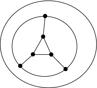
Figure 4. The limpet subgraph

xx If a graph $G$ contains a limpet then $G$ also contains a subgraph $H$ with three vertices of attachment in $G$, where $H$ is the subgraph induced by all vertices of $G$ that are not in the $3$-cycle of the limpet. Clearly, $|H|=|G|-3$ and $H$ has 6 less edges than $G$ so if $G$ is maximally independent then H is also maximally independent. If $|G|=6$, then $G$ is the doublet. If $|G|>6$, then $H$ is a proper vertex-induced subgraph of $G$ with $3$ vertices of attachment that is maximally independent.

The blocking role of the limpet should be clear by observing that attaching the limpet by two vertices of attachment to any contractible edge in a $3$-connected graph and assigning the third vertex of attachment to any other vertex gives a $3$-connected graph for which the result of contracting that same edge is definitely not $3$-connected. This is shown in Figure 5. By adding limpets into a graph in this way it is easy to generate graphs, all of whose contractible edges produce graphs that are not $3$-connected. Case (ii) of Theorem 4.1 is needed to deal with limpets.

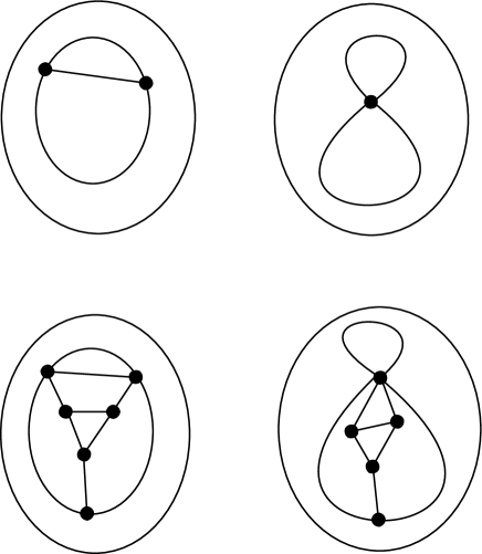
Figure 5. Adding a limpet subgraph to an edge contraction.

We are now in a position to prove the main theorem of this section using the sequence of lemmas proved below. To give some motivation to these lemmas we begin with the proof of the main theorem.

Proof of Theorem 4.1. Suppose that $G$ has no proper vertex-induced subgraph with three vertices of attachment that is maximally independent.

Assume for the sake of a proof by contradiction that $G$ contains no edge $e$ such that $G/e$ is $3$-connected and maximally independent.

$G$ is not the doublet because $|G|>6$ and $G$ has no limpets because it is maximally independent and has no proper vertex-induced subgraph which is maximally independent with three vertices of attachment.

By Lemma 4.7, $G$ has no degree $3$-vertex on a $3$-cycle.

By the Corollary 4.12, $G$ contains an edge $e$ joining vertices $x$ and $y$ such that $G/e$ is maximally independent. Then $G/e$ is not $3$-connected, by the assumption, and by Lemma 4.17, $G$ has a $3$-vertex separation set $(x,y,w)$ for some $w$, and this set separates $G$ into 2 proper components $H_{1}$ and $H_{2}$. Let $H=H_{1}$ if $|H_{1}|<|H_{2}|$ otherwise $H=H_{2}$. Now chose $e$ in $G$ which gives a minimal value for $|H|$.

By Lemmas 4.17 and 4.16 , the subgraph $H$ contains an edge $k$ which is internal to $H$ and which is contractible as an edge in $G$. Thus $G/k$ is not $3$-connected by the assumption. By Lemma 4.18, $k$ generates a $3$ vertex separation set which has one proper component properly contained in $H$. This contradicts the minimal condition on $|H|$ and completes the proof. $\Box$

This proof requires a number of lemmas which deal with the effect of an edge contraction on both maximal independence and $3$-connectivity. The apparent complexity of the proof, including the lemmas, is a result of the need to find edge contractions which maintain both of these properties simultaneously.

The first three lemmas give some useful properties of maximally independent graphs and subgraphs.

Lemma 4.2.

Let $H_{1}$ and $H_{2}$ be maximally independent subgraphs of an independent graph $G$ with $|H_{1}\cap H_{2}|\geq 2$. Then $H_{1}\cup H_{2}$ and $H_{1}\cap H_{2}$ are both maximally independent.

Proof.

$H_{1}\cup H_{2}$ and $H_{1}\cap{H_{2}}$ are both subgraphs of $G$ so they are both independent. Let $H_{1}$, $H_{2}$, $H_{1}\cup H_{2}$ and $H_{1}\cap{H_{2}}$ have $v_{1}$, $v_{2}$, $v_{u}$, $v_{i}$ and $e_{1}$, $e_{2}$, $e_{u}$, $e_{i}$ vertices and edges respectively. We have

$$2v_{1}-e_{1}-3=0,2v_{2}-e_{2}-3=0,v_{u}=v_{1}+v_{2}-v_{i},e_{u}=e_{1}+e_{2}-e_{i}.$$

Thus free$(H_{1}\cup H_{2})=2v_{u}-e_{u}-3=3-2v_{i}+e_{i}=-$ free$(H_{1}\cap H_{2})$.

Since both $H_{1}\cup H_{2}$ and $H_{1}\cap{H_{2}}$ are independent they both have freedom numbers greater than or equal to zero and thus equal to zero. ∎

Lemma 4.3.

Let $G$ be a maximally independent graph. Then $G$ is $2$-connected.

Proof.

Suppose to the contrary. Then there exist vertex-induced subgraphs $H_{1}$ and $H_{2}$ such that $G=H_{1}\cup H_{2}$ and $|H_{1}\cap H_{2}|=1$. Using the same notation as for Lemma 4.2 we have

$$free(G)=2v_{u}-e_{u}-3\geq 2(v_{1}+v_{2}-1)-e_{1}-e_{2}-3=1,$$

which contradicts the fact that $G$ is maximally independent. ∎

Lemma 4.4.

Let $G$ be a maximally independent graph. Then for any edge $e$ the contraction $G/e$ has at most one separation vertex.

Proof.

Suppose the edge $e$ joins vertices $(x,y)$ in $G$ which become the vertex $w$ in $G/e$. Then any separation vertex of $G/e$ which is different from $w$ is also a separation vertex of $G$ contrary to Lemma 4.3. ∎

The next lemma gives a useful criterion for an edge to be contractible.

Lemma 4.5.

Let $G$ be an independent graph. An edge $e=(xy)$ of $G$ is contractible if and only if

• $e$ is on exactly one $3$-cycle $(x,y,z$) of $G$ , and

• there is no maximally independent subgraph $R$ of $G$, $|R|\geq 3$, such that $x$ and $y$ are in $R$ and $z$ is not in $R$.

The condition (i) can be replaced with weaker condition $(i^{\prime})$ $e$ is on one or more $3$-cycles of $G$.

Proof.

By definition e is contractible if and only if free$(G/e)=free(G)$ and $G/e$ is independent. We show that the first of these conditions is equivalent to (i) and the second equivalent to (ii).

If $e$ is on $c$ $3$-cycles then free$(G/e)=free(G)+c+1-2$, so free$(G/e)=free(G)$ if and only if $c=1$.

Now suppose (i) is true and (ii) is false. Then there is a maximally independent subgraph $R$ of $G$ such that $x$,$y$ are in $R$ and $z$ is not in $R$. We have free$(R)=0$ and $R$ contains $e$, but not $z$. Thus free$(R/e)=-1$ (because $R$ contains no $3$-cycle containing $e$) so $G/e$ is not independent.

Conversely, suppose $G/e$ is not independent. Then $G/e$ contains a subgraph, say $R/e$, with free$(R/e)=-1$ (since contracting an edge reduces free$(H)$ by at most $1$ for any subgraph $H$ of $G$). $R/e$ must contain the edge $e$ (or $R/e$ would also be a subgraph of $G$) so $R/e$ does indeed derive from a subgraph $R$ in $G$ following contraction of $e$. Thus $R$ contains vertices $x$ and $y$ and free$(R)=0$. The vertex $z$ cannot be in $R$ because this would give free$(R/e)=0$.

Clearly (i) implies $(i^{\prime})$. Also $(i^{\prime})$ and (ii) imply (i) because if $e$ is on two or more $3$-cycles then one of these contains a vertex $w$ different from $z$ and the $3$-cycle $(w,x,y)$ gives a subgraph $R$ which violates (ii). ∎

The next lemma is standard graph theory [3] and describes what happens if the result of an edge contraction in a 3-connected graph is not $3$-connected.

Lemma 4.6.

Let $G$ be a $3$-connected graph. For any edge $e$ joining vertices $x$ and $y$, either $G/e$ is $3$-connected or $G$ has a $3$ vertex separation set consisting of $x$, $y$ and another vertex $w$ of $G$.

Proof.

Let $v$ be the vertex in $G/e$ that results from contracting e and identifying x and y in G. If $G/e$ is not 3-connected then it contains a separation pair $(a,w)$ and $a=v$ because $G$ is 3-connected. Thus $(v,w$) separate $G/e$ for some $w$ and $(x,y,w)$ separates $G$. ∎

The next lemma identifies a class of $3$-connected independent graphs that always have a contractible edge whose contraction gives a $3$-connected graph. These are graphs that contain a $3$-cycle with one or two vertices with degree $3$. Eliminating these graphs is helpful because the remaining graphs with a $3$-cycle either contain a limpet or have all vertices on the 3-cycle with at least two additional neighbours.

Lemma 4.7.

Let $G$ be a 3-connected, independent graph with no contractible edges whose contraction gives a 3-connected graph. Then any 3-cycle in $G$ either has all its vertices with degree-3 or none of its vertices with degree-3.

Proof.

Suppose that $G$ contains a $3$-cycle $(x,y,z)$ with $\deg(x)=3$. Let the third neighbour of $x$ be $t$. We will show that $\deg(y)=\deg(z)=3$.

We claim that both $(xy$) and $(xz)$ are contractible.

Suppose that neither $(xy)$ nor $(xz)$ is contractible. By Lemma 4.5 there is a maximally independent subgraph $R_{xy}$ containing $(xy)$ and not containing $z$ with $|R_{xy}|\geq 3$ and a maximally independent subgraph $R_{xz}$ containing $(xz$) and not containing $y$ with $|R_{xz}|\geq 3$. By Lemma 4.3 the vertex $x$ has at least two neighbours in $R_{xy}$which must be $y$ and $t$ and at least two neighbours in $R_{xz}$ which must be $z$ and $t$. Thus $R_{xy}\cap{R_{xz}}$ contains the vertices $x$ and $t$ so $R_{xy}\cup R_{xz}$ is maximally independent by Lemma 4.2. Then the subgraph $R_{xy}\cup R_{xz}+(yz)$ has freedom number $-1$ (since $(yz)$ is in neither $R_{xy}$ nor $R_{xz}$) which contradicts the independence of $G$.

Now suppose that $(xy)$ is contractible and that $(xz)$ is not. Then $G/(xy)$ is not $3$-connected so there exists a separation set $(x,y,w)$ of $G$. Since $G$ is $3$-connected each separation component contains a vertex connected to $x$, so there are just two separation components $C_{z}$ containing $z$ and $C_{t}$ containing $t$ and $w$ is distinct from $t$ and $z$. This is shown in Figure 6. Then all paths from $x$ to $z$ in $G$ include the edge $(xz)$ or include the vertex $y$ or include both the vertices $t$ and $w$. If $(xz)$ is not contractible there exists maximally independent $R_{xz}$ which includes $x$ and $z$ but not $y$. But then all paths from $x$ to $z$ in $R_{xz}/(xz)$ include both $t$ and $w$, so $t$ and $w$ are two separation vertices for $R_{xz}/(xz)$ which contradicts Lemma 4.4.

We can now suppose that both $(xy)$ and $(xz)$ are contractible and neither $G/(xy)$ nor $G/(xz)$ is $3$-connected. Then $G$ has a separation set $(x,y,w)$ with a component $C_{t}$ which contains the vertex $t$ and not the vertex $z$. $G$ also has a separation set $(x,z,w^{\prime})$ with a component $C_{t}^{\prime}$ which contains the vertex $t$ and not the vertex $y$.

Since $t$ and $y$ are in different components of the separation set $(x,z,w^{\prime})$ all paths from $t$ to $y$ contain either $x$, $z$ or $w^{\prime}$. The vertex set $(x,y,w)$ also separates $G$ and one component $C_{t}$ contains $t$ (and not $z$) so there is a path from $t$ to $y$ which lies inside $C_{t}$. Neither $z$ nor $x$ is inside $C_{t}$ so $w^{\prime}$ is in $C_{t}$ and $w^{\prime}$ separates $y$ from $t$ inside $C_{t}$. Since $G$ is $3$-connected this implies that the vertex $y$ is connected by the single edge $(yw^{\prime})$ to $w^{\prime}$ in $C_{t}$. Similarly $w$ is in $C_{t}^{\prime}$ and the vertex $z$ is connected by the single edge $(zw)$ to $w$ in $C_{t}^{\prime}$. This is shown in Figure 7 and Figure 8.

Figure 6. $G/(xy)$ is 2-connected. The separation set $(x,y,w)$ in $G$ gives two separation components.

Figure 7. If $(x,z,w^{\prime})$ is also a separation set of $G$ then $w^{\prime}$ is in $C_{t}$ and $w^{\prime}$ is the only neighbour of $y$ in $C_{t}$

xxx

Figure 8. Demonstration that $(y,z)$ is a separation pair of $G$ if the contractions of both $(x,y)$ and $(x,z)$ are not 3-connected.

.

Suppose that $y$ has a neighbour $v$ in addition to $x$, $z$ and $w^{\prime}$. Then $v$ is not in $C_{t}$ and $v$ is not in $C_{t}^{\prime}$ because $y$ is not in $C_{t}^{\prime}$ and $v$ and $y$ are both distinct from $(x,z,w^{\prime})$. Since $t$ is in $C_{t}$ all paths from $v$ to $t$ include one on the separation set $(x,y,w)$ before any other vertices of $C_{t}$. The vertex $x$ is connected only to $z$ outside $C_{t}$ so a path including $x$ includes $z$. The vertex $w$ is separated from $v$ by the separation set $(x,z,w^{\prime})$ and of these vertices only $z$ is outside $C_{t}$, so a path including $w$ includes $z$. Then all paths from $v$ to $t$ include either $y$ or $z$, which contradicts the fact that $G$ is $3$-connected.

We conclude that $\deg(y)=3$ and similarly $\deg(z)=3$. ∎

The remaining lemmas make use of planarity in order to simplify certain decompositions and to ensure a supply of contractible edges. The first of these lemmas makes use of the Kuratowski theorem [3] to simplify the number of separation components if the result of contracting an edge is not $3$-connected.

Lemma 4.8.

Let $G$ be a $3$-connected, planar graph with a $3$-vertex separation set. Then this separation set divides $G$ into exactly 2 proper components.

Proof.

The separation set divides $G$ into at least 2 proper components by definition. Suppose for a contradiction that there are 3 or more proper separation components. Then we can identify 3 vertices $w_{1}$, $w_{2}$, and $w_{3}$ each internal to a different separation component. Let the separation set be the vertices $v_{1}$, $v_{2}$ and $v_{3}$. There are paths connecting each of the $w_{i}$ to each of the $vj$. By Menger^′s theorem, the 3 paths from a $w_{i}$ to each of the three $v_{j}$ can be selected to be internally disjoint because $G$ is $3$-connected and the paths from different $w_{i}$ to any $v_{j}$ are internally disjoint because they are in different separation components. Thus $G$ contains $K(3,3$) as a topological minor contrary to Kuratowski^′s theorem. ∎

The next two lemmas lead to the Corollary 4.12 that states that every maximally independent, planar graph has at least 3 contractible edges. Lemma 4.11 is stronger than is required for this corollary but the greater detail will be useful subsequently.

Lemma 4.9.

Let $G,|G|>2,$ be a $2$-connected planar graph with freedom number $f$. Then every planar embedding of $G$ has the property

$$2(f-1)=\Sigma_{i}(n_{i}(i-4))$$

where the embedding has $n_{i}$ faces with $i$ edges.

Proof.

Let $G$ have $n$ vertices and $e$ edges and let the planar embedding have $F$ faces. From Euler^′s relation $F+n=e+2$ and from the definition, $f=2n-e-3$ so $f=e-2F+1$. By definition $F={\Sigma_{i}(ni)}$. Each edge is in $2$ faces of the planar embedding so $2e=\Sigma_{i}(i(ni))$ and the result follows by substituting into $f=e-2F+1$. ∎

Corollary 4.10.

A maximally independent, planar graph $G,|G|>2$ contains at least one $3$-cycle.

Proof.

A maximally independent graph has $f=0$ and is $2$-connected by Lemma 4.3. Thus in Lemma 4.9 $n_{3}\geq 2$, and the boundary of one of these faces is a 3-cycle of $G$. ∎

Lemma 4.11.

Let $G$ be an independent, planar graph which contains a $3$-cycle $(x,y,z)$ and $(i,j,k)$ be any permutation of $(x,y,z)$.

• There exists a maximally independent subgraph $R_{ij}$ of $G$ with $i$ and $j$ in $R_{ij}$ and $k$ not in $R_{ij}$ such that $R_{ij}$ contains an edge $e_{ij}$ which is contractible in $G$, and

• $R_{ij}\cap R_{jk}=j$.

Proof.

Define the $R_{ij}$ as follows: If the edge $(ij)$ is contractible then $R_{ij}=(ij)$. Otherwise, by Lemma 4.5 let $R_{ij}$ be a maximally independent subgraph containing $i$ and $j$ but not $k$ with $|R_{ij}|\geq 3$. Additionally take $R_{ij}$ to be a maximal subgraph with these properties (maximal in the sense that there is no subgraph $F$ with these properties and $H\subseteq F$).

With this definition it is clear that $j$ is in $R_{ij}\cap{R_{jk}}$. If $|R_{ij}\cap{R_{jk}}|\geq 2$ then $free(R_{ij}\cup R_{jk})=0$ by Lemma 4.2. The vertices $i$ and $k$ are in $R_{ij}\cup R_{jk}$ but the edge $(ik)$ is not in $R_{ij}\cup R_{jk}$, so the subgraph $R_{ij}\cup R_{jk}+(ik)$ of $G$ would have freedom number $-1$ which contradicts the fact that $G$ is independent. Thus $|R_{ij}\cap{R_{jk}}|=1$ and $R_{ij}\cap{R_{jk}}=j$.

It remains to show that each $R_{ij}$ contains a contractible edge which we do by induction. This is true for $|G|=3$. Assume it is true for $|G|=N$.

Since every maximally independent planar graph contains a 3-cycle (Corollary 4.10) it follows from the hypotheses that every maximally independent, planar graph $R$ with $3\leq|R|\leq N$ has at least $3$ contractible edges. Thus if $(ij)$ is not contractible then each $R_{ij}$ contains at least $3$ edges which are contractible as edges in $R_{ij}$ and one of these, say edge $e_{ij}$ is different from $(ij)$.

We claim that each $e_{ij}$ is also contractible as an edge in $G$. Otherwise there exists a maximally independent subgraph $H$ in $G$, not contained in $R_{ij}$ but also containing $e_{ij}$. In fact $H\cap{R_{ij}}=e_{ij}$, because otherwise $H\cap{R_{ij}}$ would be a maximally independent subgraph of $R_{ij}$ (by Lemma 4.2), containing $e_{ij}$ with $|H\cap{R_{ij}}|\geq 3$ which contradicts the contractibility of $e_{ij}$ in $R_{ij}$. Now $H\cup R_{ij}$ is also maximally independent by Lemma 4.2 and $|H\cup R_{ij}|>|R_{ij}|$ which contradicts the maximality of $R_{ij}$ unless $k$ is in $H\cup R_{ij}$. Suppose $k$ is in $|H\cup R_{ij}|$. Then the independence of the subgraph $H\cup R_{ij}+(ik)+(jk)$ in $G$ requires $(ik)$ and $(jk$) in $H$ (since $k$ is not in $R_{ij}$). But $i$ and $j$ are in $R_{ij}$ and $H\cap{R_{ij}}=e_{ij}$ which would require $e_{ij}=(ij)$ contrary to the assumption that $e_{ij}$ and the edge $(ij)$ are distinct. ∎

Corollary 4.12.

Every maximally independent, planar graph $G$ has at least 3 contractible edges.

Proof.

This was proved in Lemma 4.11. ∎

The next lemma guarantees the existence of a contractible edge in certain subgraphs of an independent, planar graph.

Lemma 4.13.

Let $H$ be a subgraph with 3 vertices of attachment in an independent, planar graph $G$. If $H$ contains a $3$-cycle with at least one vertex internal to $H$ then $H$ has an internal edge that is contractible as an edge of $G$.

Proof.

Let the $3$-cycle be $(x,y,z)$ with internal vertex $x$. By Lemma 4.11 there exist maximally independent subgraphs $R_{xy}$ and $R_{xz}$ containing $(xy)$ and $(xz)$ respectively and each of these contains a contractible edge.

We claim that either $R_{xy}$ or $R_{xz}$ have all their edges internal to $H$. Otherwise both $R_{xy}$ and $R_{xz}$ each contain at least two vertices of attachment, since if say $R_{xy}$ contains no vertex of attachment it is internal to $H$, and if it contains one vertex of attachment then either all its edges are internal to $H$ or $R_{xy}$ contains a vertex of $G\backslash H$. Then the vertex of attachment would be a separating vertex for $R_{xy}$, which contradicts Lemma 4.3. But if $R_{xy}$ and $R_{xz}$ each contain at least two out of the three vertices of attachment then one of these vertices must be in both $R_{xy}$ and $R_{xz}$ and thus equal to the vertex $x$ since $R_{xy}\cap{R_{xz}}=x$. This contradicts the requirement that $x$ is internal to $H$. ∎

The next sequence of lemmas has implications for $3$-connected maximally independent planar graphs for which the contraction of any contractible edge gives a graph which is not $3$-connected. We have already shown that such a graph has a 3-vertex separation set with exactly two components. The critical case for the proof of theorem 4.1 is when each component has freedom number 1. The difficulty is to show that each of these components contains a $3$-cycle so that a reduction argument can be applied to the smaller of the two components. Lemma 4.9 alone is not sufficient because substituting $f=1$ into this lemma leaves the possibility that all faces have exactly $4$ edges. We exclude this possibility by showing that at least one face has at least 5 edges.

Lemma 4.14.

Let $G$ be a $3$-connected graph and let $H$ be a proper vertex-induced subgraph of $G$ with 3 vertices of attachment. If each vertex of attachment has at least $2$ neighbours in $H$ then $H$ is $2$-connected.

Proof.

Suppose to the contrary that $H$ has a separation vertex $w$. All three vertices of attachment cannot be in the same separation component of $w$ because $G$ is $2$-connected. Thus there is a separation component for $w$ which contains exactly one vertex of attachment, say $v_{1}$ and this component must be just the edge $(wv_{1})$ or else $(w,v_{1})$ would be a separation pair for $G$. This contradicts the requirement that $v_{1}$ has at least $2$ neighbours in $H$. ∎

Lemma 4.15.

Let $G$ be a $3$-connected planar, graph and let $H$ be a proper vertex-induced subgraph of $G$ with $3$ vertices of attachment and let each vertex of attachment have at least $2$ neighbours in $H$. Then a planar embedding of $G$ implies a planar embedding of $H$ and this embedding of $H$ has the three vertices of attachment in one face boundary.

Proof.

$G$ has a planar embedding and deleting $G/H$ plus any edges connected to $G/H$ gives a planar embedding of $H$. By Lemma 4.14 $H$ is $2$-connected, so the planar embedding of $H$ divides the plane into disjoint faces.

The three vertices of attachment of $H$ in $G$ are a separation set for $G$. We claim that all vertices of $G/H$ lie in the same face with respect to the embedding of $H$. By Lemma 4.8 the $3$-vertex separation set divides $G$ into exactly $2$ separation components. Thus every pair of vertices in $G/H$ is joined together by a path in $G/H$. All vertices of $G/H$ are therefore embedded in the same face of the embedding of $H$ because otherwise these paths would cross a face boundary of the embedding of $H$ and these face boundaries lie in $H$. There is a vertex of $G/H$ adjacent to each of the three separation vertices so the three separation vertices lie on this face boundary. ∎

Lemma 4.16.

Let $G$ be a $3$-connected, independent, planar graph and let $H$ be a proper vertex-induced subgraph of $G$ with $3$ vertices of attachment $(v_{1},v_{2}\mbox{ and }v_{3})$ and let each vertex of attachment have at least $2$ neighbours in $H$. If $H$ has freedom number $1$ and if $H$ contains at most one of the edges $(v_{1}v_{2})$, $(v_{2}v_{3})$ or $(v_{3}v_{1})$ then $H$ contains an edge adjacent to an interior vertex of $H$ that is contractible as an edge of $G$.

Proof.

A planar embedding of $G$ gives a planar embedding of $H$. By Lemma 4.14 $H$ is $2$-connected and by Lemma 4.15 one of the face boundaries contains $v_{1}$, $v_{2}$ and $v_{3}$. Since $H$ contains at most one of the edges $(v_{1}v_{2})$, $(v_{2}v_{3})$ or $(v_{3}v_{1})$ this face boundary has at least $5$ edges so by Lemma 4.9 with $f=1$ the embedding of $H$ has at least one face with $3$ edges and so $H$ contains a $3$-cycle. Since $H$ has at most one of the edges $(v_{1}v_{2})$, $(v_{2}v_{3})$ or $(v_{3}v_{1})$, $H$ has a $3$-cycle with an interior vertex and by Lemma 4.13 $H$ contains an edge adjacent to an interior vertex of $H$ that is contractible as an edge of $G$. ∎

Lemma 4.17.

Let $G$ be a $3$-connected, maximally independent planar graph that contains no maximally independent vertex-induced subgraph with $3$ vertices of attachment and which has no degree $3$ vertex on a $3$-cycle. For any contractible edge $e$ joining vertices $x$ and $y$, either $G/e$ is $3$-connected or $G$ has a $3$ vertex separation set consisting of $x$, $y$ and another vertex $w$ of $G$ with the following properties:

1. $G$ does not contain edges $(xw)$ or $(yw).$

2. the separation set divides $G$ into exactly $2$ proper components such that each proper component plus the edge $(xy)$ has freedom number $1$.

3. w has at least $2$ neighbours in each of the two proper components.

Proof.

Suppose $G/e$ is not $3$-connected. By Lemma 4.6 and 4.8 $G$ has a $3$-vertex separation set $(x,y,w)$ which separates $G$ into exactly $2$ proper components $C_{1}$ and $C_{2}$. Let $H_{1}=C_{1}+(xy)+(xw)^{\prime}+(yw)^{\prime}$ and $H_{2}=C_{2}+(xy)+(xw)^{\prime}+(yw)^{\prime}$ , where $(xw)^{\prime}=(xw)$ only if the edge $(xw)$ is in $G$ and similarly for $(yw)^{\prime}$. Let $G$, $H_{1}$ and $H_{2}$ have $v$, $v_{1}$, $v_{2}$ and $e$, $e_{1}$, $e_{2}$ edges and vertices respectively. Let $d=0$, $1$ or $2$ if none, one or both of $(xw)$ and $(yw)$ is in $G$ and let $H_{1}$ and $H_{2}$ have freedom numbers $f_{1}$ and $f_{2}$. We have

$$v=v_{1}+v_{2}-3,e=e_{1}+e_{2}-1-d,2v-e-3=0,$$

$$f_{1}=2v_{1}-e_{1}-3,f_{2}=2v_{2}-e_{2}-3.$$

Thus $2(v_{1}+v_{2}-3)-(e_{1}+e_{2}-1-d)-3=0$ and so $f_{1}+f_{2}=2-d$

By hypothesis neither $H_{1}$ nor $H_{2}$ is maximally independent so $f_{1}>0$ and $f_{2}>0$. This requires $f_{1}=1$, $f_{2}=1$ and $d=0$.

Suppose a component, say $C_{1}$ has only vertex $a$ adjacent to $w$. Then $H_{1}-w-(aw)$ has freedom number $0$ and $3$ vertices of attachment in $G$. $H_{1}-w-(aw)$ is not the $3$-cycle because $w$ would be a degree $3$ vertex on a $3$-cycle contrary to hypothesis so $H_{1}-w-(aw)$ is a proper maximally independent vertex-induced subgraph of $G$, contrary to hypothesis. ∎

The final lemma allows us to conclude that under certain conditions one of the separation components that can result from contracting an edge in a subgraph must lie entirely within that subgraph.

Lemma 4.18.

Let $G$ be a $3$-connected graph and let $H$ be a proper vertex-induced subgraph of $G$ with $3$ vertices of attachment $v_{1},v_{2}$ and $v_{3}$ such that $G$ has the edge $(v_{1}v_{2})$ and does not have the edge $(v_{2}v_{3})$ or the edge $(v_{1}v_{3})$ and let $v_{3}$ have at least $2$ neighbours in the subgraph induced by the vertices of $G\backslash H+v_{1}+v_{2}+v_{3}$. Then for any interior edge $e$ of $H$ either $G/e$ is $3$ connected or one of the separation components of $G/e$ is properly contained in $H$.

Proof.

Let the edge e join vertices $x$ and $y$ with vertex $x$ interior to $H$. Suppose $G\backslash e$ is not $3$-connected. By Lemma 4.6 $G$ has a $3$-vertex separation set $(x,y,w)$. See Figure 9.

We claim that $w$ is in $H$. Suppose to the contrary that $w$ is in $G\backslash H$. Since $v_{1}$ and $v_{2}$ are adjacent they are internal vertices of only one component so there is another component $C$ that has either none of $v_{1}$, $v_{2}$ or $v_{3}$ as an internal vertex or contains $v_{3}$ and not $v_{1}$ and $v_{2}$ as internal vertex. If $C$ contains none of $v_{1}$, $v_{2}$ or $v_{3}$ then there is a path in $C$ from $w$ in $G\backslash H$ to $x$ in $H$ that avoids all vertices of attachment contrary to the definition of vertices of attachment. Suppose $C$ contains $v_{3}$ as an internal vertex and not $v_{1}$ or $v_{2}$. The vertex $v_{3}$ has at least $2$ neighbours in $G\backslash H$ (because it has at least $2$ neighbours in $G\backslash H+v_{1}+v_{2}+v_{3}$ and $G$ does not contain $(v_{1}v_{3})$ or $(v_{2}v_{3})$) so there is a vertex $u$ in $G\backslash H$ that is a neighbour of $v_{3}$ and is different from $w$. See Figure 10. Thus $u$ is in $(G\backslash H)\cap{C}$ and is different from $v_{1}$, $v_{2}$, $x$, $y$ and $w$. One of the vertices $v_{1}$ or $v_{2}$, say $v_{1}$ is not $x$ or $y$ and is thus in $G\backslash C$. Now all paths from $u$ to $v_{1}$ include one of $w$,$x$ or $y$ before any vertices in $G\backslash C$. All paths in $C$ from $u$ to $x$ or $y$ contain $v_{3}$ and thus all paths from $u$ to $v_{1}$ contain $v_{3}$ or $w$ contradicting the fact that $G$ is $3$-connected.

Now $x$, $y$ and $w$ are in $H$ and one vertex of attachment, say $v_{1}$ is different from $x,y$ and $w$. All vertices in $G\backslash H$ are connected on paths excluding $x$, $y$ and $w$ so one separation component contains at least $G\backslash H+v_{1}$ as internal vertices and so the other component is properly contained in $H$. ∎

Figure 9. The subgraph $H$ with 3 vertices of connection in $G$. There are two different placings for an interior edge $e=(x,y)$ with $x$ interior.

.

Figure 10. The hypothetical structure of the separation component $C$ if $\omega$ is in $G\backslash H$. The vertex $y$ may be identical to $v_{1}$ or $v_{2}$.

.

5. Elimination ideals and specialisation

In the present section we obtain irreducibility and divisibility properties for generators of univariate elimination ideals and their specialisations. These properties play a prominent role in the heart of our proof of the reduction step in that they connect the radical solvability of generic equations with the radical solubility of the specialised equations.

Let $f_{1},\dots,f_{r}$ be polynomials in the complex variables $\{x_{1},\dots,x_{n}\}$ which determine the complex algebraic variety $V=V(f_{1},\dots,f_{r})$ in $\mathbb{C}^{n}$. For $1\leq t<n$ the elimination ideal

$$I_{t}=\langle f_{1},\dots,f_{r}\rangle\cap\mathbb{C}[x_{1},\dots,x_{t}]$$

determines a variety $V(I_{t})$ in $\mathbb{C}^{t}$. Plainly $V(I_{t})$ contains $\pi_{t}(V)$, the projection of $V$ onto the subspace $\mathbb{C}^{t}$. The following fundamental closure theorem may be found in [4].

Theorem 5.1.

The variety $V(I_{t})$ is the Zariski closure of $\pi_{t}(V)$, that is, the smallest affine variety containing $\pi_{t}(V)$.

Let $\{d\}=\{d_{1},\dots,d_{r}\}$ be complex numbers forming an algebricaly independent set with field extension $\mathbb{Q}(\{d\})$.

Theorem 5.2.

Let $\{f\}$ be a set of polynomials in ${\mathbb{Q}}[d_{1},\ldots,d_{r}][\{x\}]$ which generates an ideal $I$ in $\mathbb{C}[\{x\}]$ whose complex variety $V(I)$ has dimension zero. Then each elimination ideal

$$I_{x_{i}}=I\cap\mathbb{C}[x_{i}],$$

for $i=1,\ldots,n$, is generated by a polynomial $g_{i}$ with coefficients in ${\mathbb{Q}}[d_{1},\ldots,d_{r}]$ and $\deg(g_{i})>0$. If, in addition, the set $\{f\}$ generates a prime ideal in the polynomial ring ${\mathbb{Q}}[d_{1},\ldots,d_{r},x_{1},\ldots,x_{n}]$ then each $g_{i}$ may be chosen to be irreducible in ${\mathbb{Q}}[d_{1},\ldots,d_{r},x_{i}]$.

Proof.

Let $\hat{I}$ denote the ideal in ${\mathbb{Q}}(\{d_{i}\})[x_{1},\dots,x_{n}]$ generated by $\{f\}$ with elimination ideals

$$(\hat{I})_{x_{i}}=\hat{I}\cap\mathbb{Q}(\{d\})[x_{i}].$$

Plainly, with the given inclusion $\mathbb{Q}(\{d\})\subseteq\mathbb{C}$ we have $\hat{I}\subseteq I$ and $I$ is the ideal in $\mathbb{C}[x_{1},\dots,x_{n}]$ generated by $\hat{I}$.

Since $(\hat{I})_{x_{i}}$ is an ideal in ${\mathbb{Q}}(\{d\})[x_{i}]$ it is generated by a single polynomial $g_{i}$, which is unique up to a nonzero multiplier in ${\mathbb{Q}}(\{d\})$. Since $V(I)$ is nonempty $g_{i}$ is not a nonzero constant, and so if deg$(g_{i})=0$ then $g_{i}=0$, and $(\hat{I})_{x_{i}}=\{0\}$. However, in this case we deduce that $I_{x_{i}}=\{0\}.$ This follows, for example, from the fact that a basis for $I_{x_{i}}$ may be derived from the generators of $I$ by algebraic operations and so lie in $(\hat{I})_{x_{i}}$. (Consider a Groebner basis construction for example.) It now follows that $V(I_{x_{i}})={\mathbb{C}}$ and the closure theorem implies that the projection $\pi_{x_{i}}(V)$ of $V(I)$ onto ${\mathbb{C}}_{x_{i}}$ is infinite and hence that $V(I)$ is infinite, contrary to hypothesis. Thus deg$(g_{i})>0$.

The coefficients of $g_{i}$ are in ${\mathbb{Q}}(\{d\})$ and so are ratios of polynomials in ${\mathbb{Q}}[\{d\}]$. Thus we may replace $g_{i}$ by $p(d_{1},...,d_{r})g_{i}$ for some polynomial $p$ to obtain the desired generator with polynomial coefficients. We may also arrange that the highest common factor of the coefficients of $g_{i}$ is $1$.

We claim that the generator $g_{i}$, when viewed as an element of the ring ${\mathbb{Q}}[\{d\},\{x_{i}\}]$, is also a generator for the polynomial ring elimination ideal

$$J_{x_{i}}=J\cap{\mathbb{Q}}[\{d\},x_{i}],$$

where $J$ is the ideal in $\mathbb{Q}[\{d\},\{x\}]$ generated by $\{f\}$.

Let $h\in J_{x_{i}}$. Then $h$ is also in $(\hat{I})_{x_{i}}$ and so $h=qg_{i}$ with $q$ in ${\mathbb{Q}}(\{d\})[x_{i}]$. Clearing the denominators of the coefficients of $q$ obtain the factorisation $r(d_{1},...,d_{r})h=(r(d_{1},...,d_{r})q)g_{i}$ where $r(d_{1},...,d_{r})$ is in ${\mathbb{Q}}[\{d\}]$ and $r(d_{1},...,d_{r})q$ is in ${\mathbb{Q}}[\{d\}][x_{i}]$. Since, by the hypotheses, the ideal $J$ is prime, so too is $J_{x_{i}}$ and so one of these factors belongs to $J_{x_{i}}$. However, if $r(d_{1},...,d_{r})q$ belongs to $J_{x_{i}}$ then we can repeat the factorisation argument with $r(d_{1},...,d_{r})q$ in place of $h$. Factoring in this way at most finitely many times we see that we can assume that $h$ has the form $pg_{i}$ with $p$ in ${\mathbb{Q}}(\{d\})[x_{i}]$. Since the coefficients of $g_{i}$ have no common factor it follows that $p$ is in ${\mathbb{Q}}[\{d\}][x_{i}]$ and that $g_{i}$ is a generator for $J_{x_{i}}$. Since $J_{x_{i}}$ is prime this in turn entails that the generator $g_{i}$ is irreducible in ${\mathbb{Q}}[\{d\},\{x_{i}\}]$. ∎

We now show that in the case $r=0$ the specialised generator $g(d^{\prime},x_{i})$ is non-zero and divisible by the generator $g_{i}(x_{i})$ of the elimination ideal of the specialised ideal. As we note below, such divisibility may fail for a double specialisation !

For later convenience the role of $\mathbb{Q}$ in the theorem above is played below by $\mathbb{E}\subseteq\mathbb{C},$ a finite transcendental field extension of $\mathbb{Q}$. (It is trivial to generalise the theorem above with $\mathbb{Q}$ replaced by $\mathbb{E}$.) Specialisation occurs for the single variable $d$ associated with the transcendental extension $\mathbb{E}(d)$. For an ideal $\hat{I}$ in $\mathbb{E}[d][x_{1},...,x_{n}]$ we shall write $(\hat{I})^{\prime}$ for the specialisation of $\hat{I}$ resulting from the substitution $d\to d^{\prime}$.

Theorem 5.3.

Let $\{f\}$ be a set of polynomials in ${\mathbb{E}}[d][x_{1},\ldots,x_{n}]$ which generate an ideal $\hat{I}$ in ${\mathbb{E}}(d)[x_{1},\ldots,x_{n}]$ and an ideal $I$ in $\mathbb{C}[x_{1},\ldots,x_{n}]$ whose complex variety $V(I)$ has dimension zero. Let $d^{\prime}\in{\mathbb{Q}}$ be a specialisation of $d$ giving rise to the set $\{f^{\prime}\}$ in ${\mathbb{E}}[x_{1},\ldots,x_{n}]$ with ideal $I^{\prime}$ whose complex variety also has dimension zero.

Let $g(d,x_{1})$ in ${\mathbb{E}}[d][x_{1}]$ and $g^{\prime}(x_{1})$ in ${\mathbb{E}}[x_{1}]$ be generators for the elimination ideals $I_{x_{1}}$ and $(I^{\prime})_{x_{1}}$ respectively, as provided by the previous theorem. Finally, assume that the ideal in $\mathbb{E}[d,x_{1},\dots,x_{n}]$ generated by $\{f\}$ is prime. Then

(i) the specialisation $((\hat{I})_{x_{1}})^{\prime}$ of $(\hat{I})_{x_{1}}$, is contained in $((\hat{I})^{\prime})_{x_{1}}$,

(ii) the degree of $g(d^{\prime},x_{1})$ is greater than zero, and

(iii) $g^{\prime}(x_{1})$ divides $g(d^{\prime},x_{1})$.

Proof.

We have

$$((\hat{I})_{x_{1}})^{\prime}=\{p(d^{\prime},x_{1}):p\in\hat{I}\cap{\mathbb{E}}(d)[x_{1}]\}.$$

But if $p(d,x_{1})\in\hat{I}$ then $p(d^{\prime},x_{1})\in(\hat{I})^{\prime}$ and so $((\hat{I})_{x_{1}})^{\prime}\subseteq((\hat{I})^{\prime})_{x_{1}}$. Thus if $g(d^{\prime},x_{1})$ is not the zero polynomial then $g^{\prime}(x_{1})$ divides $g(d^{\prime},x_{1})$ and deg($g(d^{\prime},x_{1}))>0$.

Let $J$ be the ideal in ${\mathbb{E}}[d,x_{1},...,x_{n}]$ generated by $\{f\}$ and let $J_{d,x_{1}}$ be the elimination ideal $J\cap{\mathbb{E}}[d,x_{1}]$. Then $J_{d,x_{1}}$ has generator $g_{1}(d,x_{1})$ where this polynomial is the generator of $(\hat{I})_{x_{1}}$ in ${\mathbb{E}}(d)[x_{1}]$ provided by the previous theorem. By this theorem we may assume that $g_{1}(d,x_{1})$ is irreducible in ${\mathbb{E}}[d,x_{1}]$. In this case it is not possible to have $g_{1}(d^{\prime},x_{1})=0$ for all $x_{1}$, for otherwise $g_{1}$ would have a proper factor $(d-d^{\prime})$. ∎

It is instructive to note that Theorem 5.3 is not valid without the assumption that the big ideal is prime. Consider the equation set

$$(dx-1)p(x)=0,~{}~{}~{}~{}d(dx-1)=0,$$

where $p(x)$ is a polynomial in one variable $x$ over $\mathbb{Q}$ and $d$ is a single parameter. For generic $d$ the ideal $I=\langle(dx-1)p(x),d(dx-1)\rangle$ in $\mathbb{Q}[x]$ is the principal ideal $\langle dx-1\rangle,V(I)$ is the singleton $\{1/d\}$ and  dim$(V(I))=0$. For the specialisation $d=0$ the ideal for the specialised equations is $I^{\prime}=\langle p(x)\rangle$ and $V(I^{\prime})$ is the finite set of zeros of $p$ and so is also zero dimensional. However, it is not possible to choose a generator for $I^{\prime}$ which divides a nonzero generator of $I$, and so the conclusion of Theorem 5.3 cannot hold for this equation set.

Note also that in this example we may choose $p(x)$ to be a polynomial which is not soluble over $\mathbb{Q}$ so that while the generic variety $V(I)$ is radical the variety for the specialised equations is not radical.

It is also instructive to note that Theorem 5.3 is not valid for the specialisation of more than one parameter. For example, let

$$f_{1}=x_{1}(1-x_{1}x_{2})-d_{1},f_{2}=x_{2}(1-x_{1}x_{2})-d_{2},f_{3}=x_{3}(1-x_{1}x_{2})-d_{3}.$$

For the double specialisation $d_{1}=d_{2}=0,V(I^{\prime})$ is the single point $x_{1}=0,x_{2}=0,x_{3}=d_{3}$ and

$$g_{1}(d_{1},d_{2},x_{1})=d_{2}x_{1}^{3}-d_{1}x_{1}+d_{1}^{2}$$

which becomes zero on this specialisation.

6. The reduction step

Equipped with the elimination theory of the last section we are now able to prove the reduction step stated in the introduction.

Let $G$ be a maximally independent graph with $n$ vertices and $r+1$ edges and suppose that $G$ has an edge contraction to a maximally independent graph $G/e$. We label the vertices so that $e$ is the edge $(v_{n-1}v_{n-2}),e$ is in the 3-cycle $(v_{n},v_{n-1},v_{n-2})$ and we regard $(v_{n-1}v_{n})$ as the base edge. Furthermore, we normalise the constraint equations $\{f_{e}\}$ so that the coordinates for the base vertices are $(x_{n-1},y_{n-1})=(0,0),(x_{n},y_{n})=(1,0)$. Let us label edges so that the contractible edge e is the rth edge, with the associated (squared) dimension $d_{r}$, and the edge $(v_{n-2}v_{n})$ has dimension $d_{r-1}$. Finally let $f_{1},...,f_{r}$ be a listing of the normalised constraint equations for $G$ compatible with this notation.

Now consider a set of normalised constraint equations for the contracted graph $G/e$. We lose two edges from $G$ (edge $r-1$ and edge $r$) and we can take the normalised constraint equations to be the equations $f_{1},\dots f_{r-2}$ with the substitution $x_{n-2}=0$, $y_{n-2}=0$.

First consider the dimensions $\{d\}=\{d_{1},\dots,d_{r-2}\}$ (together with $d_{b}=1$) to be a generic set of real numbers. Since the contracted graph is maximally independent the solutions (for $x_{1},\dots,x_{n-3},y_{1},\dots,y_{n-3}$) form a zero dimensional variety, $V(0,0)$ say. (The choice of notation will become clear shortly.) Clearly this is essentially the variety of the constraint equations $\{f_{1},\dots,f_{r}\}$ for the dimension set

$$\{d_{1},\dots,d_{r-1},d_{r-2},1,0\}$$

for $G$ resulting from the double specialisation $d_{r-1}=1,d_{r}=0.$ Thus, in order to establish the reduction step it will be sufficient to show that if $G$ is generically radical then the variety arising from the semi-generic double specialisation is also a radical variety. This requires some care in view of the failure of a double specialisation variant of the Theorem 5.3. We shall break the double specialisation into two steps. Also, instead of specialising the generic edge lengths $d_{r},d_{r-1}$ we choose to start afresh and specialise the given coordinates $x_{n-2},y_{n-2}$. This results in a simpler comparison of varieties.

In fact we can prove the reduction step for general non-planar graphs.

Theorem 6.1.

Let $G$ be a maximally independent graph which has an edge contraction to a maximally independent graph $G/e$. If $G$ is radically soluble then the graph $G/e$ is also radically soluble.

Proof.

Consider the set of dimensions $\{d\}=\{d_{1},\dots,d_{r-2}\}$ and the constraint equations $\{f_{1},\dots,f_{r-2}\}$ in the variables $x_{1},\dots x_{n-3}$, $y_{1},\dots,y_{n-3}$ which arise when the pair $(x_{n-2},y_{n-2})$ takes three possible pairs of values, namely $(X,Y),(X,0)$ and $(0,0)$, where $X,Y$ are generic. Denote the three corresponding ”big” varieties, where $\{d\}$ is a set of variables, by $V_{b}(X,Y))$, $V_{b}(X,0)$ and $V_{b}(0,0)$. For generic values of $\{d\}$ let the corresponding ”small” varieties be $V(X,Y))$, $V(X,0)$ and $V(0,0)$. Also we write $I_{b}(X,Y),I(X,Y)$ etc., for the six corresponding ideals

We have the following:

1. The varieties $V_{b}(X,Y))$, $V_{b}(X,0)$ and $V_{b}(0,0)$ are irreducible. This follows from the fact that the equations are parametric in the variables. See Theorem 2.8.

2. The variety $V(0,0)$ is zero dimensional by Theorem 2.4 because it is the variety of the maximally independent generic graph $G/e$. The varieties $V(X,0)$ and $V(X,Y)$ also have the form required for Theorem 2.3. The determinant of the Jacobian matrix for $V(0,0)$ is obtained from the corresponding determinants for $V(X,0)$ and $V(X,Y)$ by substituting $X=0$ and $Y=0$ and thus neither of the determinants of the Jacobian matrices for $V(X,0)$ and $V(X,Y)$ are identically zero. Then $V(X,0)$ and $V(X,Y)$ are zero dimensional by Theorem 2.3.

We may now apply the specialisation theorem of Section 5 two times, once for the specialisation $(X,0)\to(0,0)$ and once for the specialisation $(X,Y)\to(X,0)$.

Suppose then, that $V(0,0)$ is non-radical. In fact assume that there is a point of this variety whose $x$-coordinate is not in a radical extension of $\mathbb{Q}(\{d\})$. Since $V_{b}(0,0)$ is irreducible and $V(0,0)$ is zero dimensional, it follows from Theorem 5.2 that there exists a univariate polynomial $g(x_{i})$ in $\mathbb{Q}(\{d\})[x_{i}]$ which generates the elimination ideal $I(0,0)_{x_{i}}$. By the closure theorem, Theorem 5.1, $\pi_{x_{i}}(V(0,0))$ is precisely the variety of the elimination ideal for $x_{i}$ and this is precisely the set of zeros of $g_{i}$. By the non-radical hypothesis there exists an $x_{i}$ such that $g_{i}$ has some of its roots non-radical (over $\mathbb{Q}(\{d\})$). By irreducibility, all the roots are non-radical.

Likewise, $V(X,0)$ is zero dimensional and there exists a polynomial $g(x_{i},X)$, with positive degree in $x_{i}$, which generates $I(X,0)_{x_{i}}$. Moreover, since $V_{b}(X,0)$ is irreducible we may choose $g$ so that $g(x_{i},X)$ is not divisible by $X$ and hence $g(x_{i},0)$ is not identically zero. But $g(x_{i},0)$ is in $I(0,0)_{{xi}}$ and so $g(x_{i})$ divides $g(x_{i},0)$. Thus $g(x_{i},0)$ has a non-radical root, $g(x_{i},0)$ is non-radical and $V(X,0)$ is non-radical.

Repeating this argument for $V(X,0)$ and $V(X,Y)$ shows that $V(X,Y)$ is non-radical over $\mathbb{Q}(\{d\})$. Thus $V$ is non-radical over $\mathbb{Q}(\{d\},X,Y).$ However, by triangle geometry $X$ and $Y$ are radical functions of $d_{r-1}$ and $d_{r}$. Thus $V$ is non-radical over $\mathbb{Q}(d_{1},...,d_{r}).$ ∎

Remark. One needs to take care with simultaneous specialisation. If we do both specialisations together on $V(X,Y)$ we might have

$$g(x_{i},X,Y)=Xp(x_{i},X,Y)+Yq(x_{i},X,Y),$$

where, for example, $Y$ does not divide $p$ and so $g(x_{i},0,0)=0,$ which gives no information on divisibility. In fact we have not excluded this possibility by doing the specialisations one at a time. However we have shown that if this does occur then $p$ and $q$ both have factors which are non-radical. This is sufficient to deduce that $g(x_{i},X,Y)$ is non-radical, even if it is zero on the double specialisation.

7. Galois group under specialisation

We now obtain a theorem concerning the Galois groups of polynomials whose coefficients contain indeterminates which may be specialised. This theorem plays a role in the proof of the fact that if the graph $G$ is soluble by radicals for generic dimensions then it is also soluble by radicals for certain specialised dimensions. In the proof we make use of the identification of the Galois group of $p$ as the set of permutations in an index set associated with a certain irreducible factor of a multi-variable polynomial constructed from $p$. This identification is well-known and given in Stewart [13].

Let ${d}=\{d_{1},\dots,d_{n}\}$ be algebraically independent variables with the rational field extension $\mathbb{Q}({d})$ and let ${d^{\prime}}=\{d_{1}^{\prime},\dots,d_{n}^{\prime}\}$ be an $n$-tuple of rationals, viewed as a specialisation of ${d}$.

Theorem 7.1.

Let $p\in{\mathbb{Q}}[{d}][t]$ be an irreducible monic polynomial with Galois group   Gal$(p)$ when viewed as a polynomial in ${\mathbb{Q}}({d})[t]$. Let ${d}^{\prime}\in{\mathbb{Q}}^{n}$ be a specialisation of  ${d}$ and let  $p^{\prime}$ be the associated specialisation of $p$ with Galois group Gal$(p^{\prime})$ over ${\mathbb{Q}}$. Then Gal$(p^{\prime})$ is a subgroup of Gal$(p)$. In particular if $p$ is a radical polynomial then so too is $p^{\prime}$.

Proof.

Consider the irreducible polynomial

$$p(t)=t^{m}+b_{m-1}({d})t^{m-1}+\ldots+b_{0}({d})$$

with coefficients $b_{i}({d})$ in ${\mathbb{Q}}[{d}]$. Let $\alpha_{1},\ldots,\alpha_{m}$ be the roots of $p(t)$ in some splitting field, let $\{x_{1},\ldots,x_{m}\}$ be indeterminates and let

$$\beta=\alpha_{1}x_{1}+\ldots+\alpha_{m}x_{m}.$$

Let $S_{m}$ be the symmetric group and define

$$Q(t,x_{1},\ldots,x_{m})=\prod_{\sigma\in S_{m}}\left(t-\sigma(\beta)\right)$$

where $\sigma(\beta)=\alpha_{1}x_{\sigma(1)}+\ldots+\alpha_{m}x_{\sigma(m)}$. On expanding the product it can be seen that the coefficient of a monomial $t^{k}{x_{1}}^{{i_{1}}}{x_{2}}^{{i_{2}}},\dots,{x_{m}}^{{i_{m}}}$ is a symmetric polynomial in the roots $\alpha_{i}$. It follows that these coefficients are polynomials in $b_{m-1}({d}),\ldots,b_{0}({d})$. (See [13].) Thus the polynomial $Q$ belongs to ${\mathbb{Q}}[{d}][t,{x}].$

Let $Q=Q_{1}Q_{2}\ldots Q_{r}$ where each $Q_{i}$ is irreducible in ${\mathbb{Q}}[{d}][t,x]$ and where $Q_{1}$ contains the factor $(t-\beta)$. Since the roots of an irreducible polynomial are distinct so too are the expressions $\sigma(\beta)$ and it follows that the polynomial $Q_{1}$ is well-defined.

We have

$$Q_{1}=\prod_{\sigma\in S}(t-\sigma(\beta))$$

for some index set $S$. This index set is a subgroup of $S_{m}$ which is identifiable with the Galois group of $p$. It coincides with the group of permutations $\sigma$ of the variables $x_{1}\ldots,x_{m}$ for which $\sigma(Q_{1})=Q_{1}$. In fact each $Q_{i}$ has the form $\tau(Q_{1})$ for some permutation $\tau$ and from this it follows that if $\sigma(Q_{i})=Q_{i}$ for some $i$ then this holds true for all $i$ and $\sigma$ is in the Galois group.

Now consider the specialisation $Q^{\prime}$ of the polynomial $Q$ in $~{}{\mathbb{Q}}[{d}][t,{x}]$ upon replacing ${d}$ by ${d^{\prime}}$. Since the coefficients of $Q$ are polynomials in $b_{m-1}({d}),\ldots,b_{0}({d})$ it is easy to see that $Q^{\prime}$ coincides with the ’$Q$ polynomial’ for $p^{\prime}$. Thus $Q^{\prime}$ is equal to the polynomial

$$\prod_{\sigma\in S_{m}}~{}\left(t-\sigma(\beta^{\prime})\right)$$

where $\beta^{\prime}=\alpha_{1}^{\prime}x_{1}+\ldots+\alpha_{m}^{\prime}x_{m}$ and $\alpha_{1}^{\prime},\ldots,\alpha_{m}^{\prime}$ are the roots of the specialisation $p^{\prime}$ in some order. (Despite the notation we do not imply that there is a link between any $\alpha_{i}^{\prime}$ and $\alpha_{i}$.)

Note that for any permutation $\sigma$ and polynomial $P$ in ${\mathbb{Q}}[{d}][t,{x}]$ the polynomial $\sigma(P)$ is defined by permuting the indeterminates $x_{1},\ldots,x_{m}$. Thus $\sigma(P)^{\prime}=\sigma(P^{\prime})$, which is to say that the permutation action on these polynomials commutes with specialisation.

Consider now both the specialisation of the factorisation, namely

$$Q^{\prime}=Q_{1}^{\prime}Q_{2}^{\prime}\ldots Q_{r}^{\prime},$$

and the irreducible factorisation of $Q^{\prime}$ in ${\mathbb{Q}}[t,{x}]$, namely

$$Q^{\prime}=P_{1}P_{2}\ldots P_{s}.$$

Let us assume first that the roots $\alpha_{i}^{\prime}$ are distinct. Then, since each $P_{i}$ is necessarily a product of some of the irreducible factors $t-\sigma(\beta^{\prime})$, there is a unique factor, $P_{1}$ say, divisible by $t-\beta^{\prime}$. Once again (and even though $p^{\prime}$ may be reducible) the Galois group $Gal(p^{\prime})$ is identifiable with $T$ where $T\subseteq S_{m}$ is the index set such that

$$P_{1}=\prod_{\sigma\in T}(t-\sigma(\beta^{\prime})).$$

The roots $\alpha_{1}^{\prime},\ldots,\alpha_{m}^{\prime}$ do not correspond to $\alpha_{1},\ldots,\alpha_{m}$ and so we cannot assume that $P_{1}$ divides $Q_{1}^{\prime}.$ (Such divisibility gives $T\subseteq S$ and so completes the proof in this case.) However, let $\sigma\in T$, so that $\sigma(P_{1})=P_{1}$, and suppose that $P_{1}$ divides $Q_{i}^{\prime}$. Then $P_{1}$ divides $\sigma(Q_{i}^{\prime})=\sigma(Q_{i})^{\prime}=Q_{j}^{\prime}$ say, where $Q_{j}=\sigma(Q_{i})$. By the distinctness of the roots $\alpha_{i}^{\prime}$ and the fact that $\mathbb{Q}[t,x]$ is a unique factorisation domain, it follows that if $P_{1}$ divides both $Q_{i}^{\prime}$ and $Q_{j}^{\prime}$ then $i=j$. Thus $\sigma(Q_{i})=Q_{i}$. But by our remarks earlier this condition on $\sigma$ is equivalent to $\sigma(Q_{1})=Q_{1}$ and hence $\sigma\in S=Gal(p)$.

We now give more notational detail on this case which we shall elaborate further to prove the general case.

Assume that $p^{\prime}=h_{1}h_{2}\ldots h_{q}$ where $h_{1},\ldots,h_{q}$ are distinct irreducible polynomials in ${\mathbb{Q}}[t]$ with $\deg h_{i}=r_{i}$.

The Galois group $T=Gal(p^{\prime})$ can be identified in a natural way with a subgroup of the product group $Gal(h_{1})\times\dots\times Gal(h_{q})$. We remark that $T$ may be a proper subgroup. For example, if $h_{1}$ and $h_{2}$ determine the same field extension of $\mathbb{Q}$ then $r_{1}=r_{2}$ and $Gal(h_{1}h_{2})=Gal(h_{1})$. (Each permutation of the roots of $h_{1}$ determined by an element of $Gal(h_{1})$ is matched with a corresponding permutation of roots of $h_{2}$.) In general $Gal(p^{\prime})$ is a product of the Galois groups of the distinct field extensions determined by irreducible factors of $p^{\prime}$.

The irreducible polynomial $P_{1}$ above factors as a product

$$P_{1}=\prod_{\sigma=\sigma_{1}\times\ldots\times\sigma_{q}\in T}\left(t-(\sigma_{1}(\beta_{1}^{\prime})+\ldots+\sigma_{q}(\beta_{q}^{\prime})\right),$$

where $\beta_{i}^{\prime}=\alpha_{i,1}^{\prime}x_{i,1}+\ldots+\alpha_{i,r_{i}}^{\prime}x_{i,r_{i}}$, and where $\alpha_{i,1}^{\prime},\ldots,\alpha_{i_{i}r_{i}}^{\prime}$ are the distinct roots of $h_{i}$. Thus we have $r_{1}+\dots+r_{q}=m$ and we have identified the variables $x_{1},\ldots,x_{m}$ with the variables

$$x_{1,1},\ldots,x_{1,r_{1}},x_{2,1},\dots,x_{2,r_{2}},~{}~{}~{}\ldots~{}~{}~{},x_{q,1},\dots,x_{q,r_{q}}.$$

Consider now the general case wherein $p^{\prime}=h_{1}^{n_{1}}h_{2}^{n_{2}}\ldots h_{q}^{n_{q}}$ where each $h_{i}$ is as before, with degree $r_{i}$. Now each root $\alpha_{i,k}^{\prime}$ appears with multiplicity $n_{i}$ and $m$ now satisfies the equation

$$n_{1}r_{1}+\ldots+n_{q}r_{q}=m.$$

Let us accordingly relabel the variables $x_{i,j}$ as

$$\{x_{i,k,t}:1\leq i\leq q,1\leq k\leq r_{i},1\leq t\leq n_{i}\}$$

Identify each element $\sigma=\sigma_{1}\times\ldots\times\sigma_{q}$ of $T=Gal(p^{\prime})$ with the permutation in

$$(Gal(h_{1})\times\ldots\times Gal(h_{1}))\times\ldots\times(Gal(h_{q})\times\ldots\times Gal(h_{q}))$$

which respects the ordering of repeated roots and which respects the matching of permutations in $Gal(h_{i})$ and $Gal(h_{j})$ if $h_{i}$ and $h_{j}$ determine the same field extension. In this way we obtain an identification of $Gal(p^{\prime})$ as a subgroup of $S_{m}$. Note that there is a degree of choice in this identification; the permutations that permute only indices of equal roots give rise to distinct embeddings.

Consider now the polynomial in $\mathbb{Q}[t,x]$ associated with this inclusion defined by

$$P_{*}=\prod_{\sigma\in Gal(p^{\prime})\subseteq S_{m}}\left(t-\sigma(\beta^{\prime})\right).$$

This polynomial has the form $\hat{P}_{1}$ where

$$\hat{P}_{1}=P_{1}(X_{1},\ldots,X_{q})$$

where $P_{1}$ is the irreducible polynomial we had in the previous case and where each $X_{i}$ is the sum of those variables corresponding to repeated and matched roots.

Since $P_{1}$ is irreducible it follows that $\hat{P}_{1}$ is irreducible. It follows further that the irreducible factors of $Q^{\prime}$, and hence $Q_{1}^{\prime}$, have the form $\tau(\hat{P}_{1})$ for certain permutations $\tau$ in $S_{m}$, namely for a set of permutations chosen from the right cosets of the subgroup $Gal(p^{\prime})$.

Choose $\tau$ so that $t-\tau(\beta^{\prime})$ divides $P_{*}$. This means that $t-\tau(\beta^{\prime})=t-\sigma(\beta^{\prime})$ for some permutation in $Gal(p^{\prime})$ and hence that $\tau\circ\sigma^{-1}$ is a permutation that permutes the indices of repeated roots. We may now reorder the repeated roots to define a new embedding of $Gal(p^{\prime})$ so that $\tau\circ\sigma^{-1}=1.$ Thus $t-\beta^{\prime}$ is a factor of $P_{*}$ and it follows as before that $P_{*}$ divides $Q_{1}^{\prime}$ and that $T$ is a subgroup of $S$, as desired.

The last assertion of the theorem follows from the fact that a subgroup of a soluble group is soluble. (See [13].) ∎

The non-monic case of the last theorem can be deduced with the following change of variables argument.

Suppose that $p$ is an irreducible polynomial in $\mathbb{Q}[d][t]$ with non-zero specialisation $p^{\prime}$. Choose a rational number $a$ so that $p^{\prime}(a)\neq 0$, and hence $p(a)\neq 0$. Define the irreducible polynomial

$$q(z)=t^{n}p(t^{-1}+a)\frac{1}{p(a)}.$$

Then $q$ is monic with well-defined specialisation

$$q^{\prime}(t)=t^{n}p^{\prime}(t^{-1}+a)\frac{1}{p^{\prime}(a)}.$$

The splitting fields of $p$ and $q$ are isomorphic as are those of $p^{\prime}$ and $q^{\prime}$ and so it follows from the theorem above that $Gal(p^{\prime})$ is a subgroup of $Gal(p)$.

It is clear that the arguments above extend verbatim to the specialisation of algebraic independents over any field of characteristic zero and we shall need results in this setting. Let $\mathbb{E}$ be such a field and let $\{d\}$ be a set of algebraically independent variables over $\mathbb{E}$ with rational field extension $\mathbb{E}(d)$.

Theorem 7.2.

Let $p\in{\mathbb{E}}[{d}][t]$ be an irreducible polynomial with Galois group   Gal$(p)$ when viewed as a polynomial in ${\mathbb{E}}({d})[t]$. Let ${d}^{\prime}\in{\mathbb{E}}^{n}$ be a specialisation of  ${d}$ and let  $p^{\prime}$ be the associated specialisation of $p$ with Galois group Gal$(p^{\prime})$ over ${\mathbb{E}}$. If $p^{\prime}$ is non-constant then Gal$(p^{\prime})$ is a subgroup of Gal$(p)$. In particular if $p$ is a radical polynomial then so too is $p^{\prime}$.

8. Planar $3$-connected CAD graphs are non-soluble

We are now able to prove the main theorem stated in the introduction.

Suppose, by way of contradiction, that there exists a maximally independent $3$-connected planar graph which is soluble. Let $G$ be such a graph with the fewest number of vertices. We show that $G$ is the doublet graph and that the doublet graph is not soluble by radicals. This contradiction completes the proof.

By the reduction step, Theorem 6.1, the vertex minimal graph $G$ has no edge contraction to a $3$-connected maximally independent planar graph. It thus follows from the main reduction theorem for such graphs, Theorem 4.1, that either $|G|=6$, and $G$ is the doublet (since $G$ is planar), or that $G$ has a proper vertex induced maximally independent subgraph with three vertices of attachment. However minimality rules out the latter possibility because the next proposition shows that such a proper subgraph admits substitution by a smaller graph, namely a triangle, and the resulting graph is soluble if $G$ is soluble.

Proposition 8.1.

Let $G$ be a 3-connected, maximally independent graph and let H be a maximally independent subgraph of $G$ with $3$ vertices of attachment $v_{1},v_{2}$ and $v_{3}$. Let $G^{\prime}$ be the graph which is obtained from $G$ by deleting all the internal vertices of $H$ and all the edges of $H$ and adding the edges $(v_{1}v_{2}),(v_{2}v_{3}),(v_{3}v_{1}).$ Then $G^{\prime}$ has the properties:

(i) $G^{\prime}$ is $3$-connected.

(ii) $G^{\prime}$ is maximally independent.

(iii) If the dimensions in the constraint equations defined by $G$ are chosen as algebraic independents then the dimensions in the equations defined by $G^{\prime}$ are also algebraic independents.

Proof.

If $|H|=3$ then $H$ is the $3$-cycle and $G=G^{\prime}$, so assume $|H|\geq 4$. Note that $H$ is connected since otherwise $G$ is not even be $2$-connected.

Every path in $G^{\prime}$ derives from a path in $G\backslash H$ plus paths in $H$ which replaces segments $v_{i}\to v_{j}$ or $v_{i}\to v_{j}\to v_{k}$ for $v_{i},v_{j},v_{k}$ chosen from the vertices of attachment. For any set of independent paths in $G^{\prime}$, at most one of them contains any of the edges $(v_{1}v_{2}),(v_{2}v_{3})$ or $(v_{3}v_{1})$. Thus every set of independent paths in $G^{\prime}$ gives a set of independent paths in $G$ and (i) follows.

If $H_{1}$ and $H_{2}$ are any two edge disjoint subgraphs in $G$ then it follows easily from the definition of $free(H)$ that

$$free(H_{1}\cup H_{2})=free(H_{1})+free(H_{2})+3-2|H_{1}\cap H_{2}|.$$

This gives immediately that $free(G^{\prime})=0$. If $G^{\prime}$ is not independent then there is a subgraph $R$ of $G^{\prime}$ with $free(R)<0$ and there is an edge $(v_{1}v_{2})$, say, which is in $R$ but not in $G$. If $v_{3}$ is not in $R$ then $(R\backslash(v_{1}v_{2}))\cup H$ is in $G$ and $free((R\backslash(v_{1}v_{2}))\cup H)<0$ which contradicts the independence of $G$. If $v_{3}$ is in $R$ then $(R\{(v_{1}v_{2}),(v_{2}v_{3}),(v_{1}v_{3})\})\cup H$ is in $G$ and $free((R\{(v_{1}v_{2}),(v_{2}v_{3}),(v_{1}v_{3})\})\cup H)<0$ which contradicts the independence of $G$.

Theorem 2.3 implies that for algebracially independent dimensions $\{d_{i}\}$, any zero of the variety of $G$ has coordinates $\{x_{j}\}$ which are algebraically independent. This zero of the variety of $G$ gives a zero of the variety of $G^{\prime}$ (with the same $\{x_{j}\}$ where they occur and with the same $\{d_{i}\}$ where they occur and $d_{12},d_{23}$ and $d_{13}$ computed from $d_{ij}=(x_{i}-x_{j})^{2}+(y_{i}-y_{j})^{2})$ and this zero therefore has coordinates which are algebraically independent. It follows from Theorem 2.3 that the dimensions of $G^{\prime}$ are algebraically independent.

∎

We now show that the doublet is a non-soluble CAD graph.

Let $v_{1}=(0,0),v_{2}=(1,0)$ be the vertices of the base edge. Introduce the coordinates $(x_{i},y_{i})$ for the remaining vertices $v_{i},3\leq i\leq 6$, and the dimensions $d_{j},2\leq j\leq 9$, for the non-base edges. The indexing scheme is illustrated in Figure 9.

Figure 11. Coordinatisation of the doublet.

The resulting polynomials $\{f\}$ for the normalised constraint equations take the form

$$\begin{array}[]{ccccc}\vspace{2mm}x_{4}^{2}&+&y_{4}^{2}&-&d_{9}^{2}\\ \vspace{2mm}x_{5}^{2}&+&y_{5}^{2}&-&d_{8}^{2}\\ \vspace{2mm}(x_{3}-1)^{2}&+&y_{3}^{2}&-&d_{2}^{2}\\ \vspace{2mm}(x_{6}-1)^{2}&+&y_{6}^{2}&-&d_{7}^{2}\\ \vspace{2mm}(x_{3}-x_{4})^{2}&+&(y_{3}-y_{4})^{2}&-&d_{3}^{2}\\ \vspace{2mm}(x_{4}-x_{5})^{2}&+&(y_{4}-y_{5})^{2}&-&d_{4}^{2}\\ \vspace{2mm}(x_{5}-x_{6})^{2}&+&(y_{5}-y_{6})^{2}&-&d_{5}^{2}\\ \vspace{2mm}(x_{6}-x_{3})^{2}&+&(y_{6}-y_{3})^{2}&-&d_{6}^{2}.\end{array}$$

For each choice of real algebraically independent squared dimensions ${\displaystyle d_{2}^{2},\ldots,d_{9}^{2}}$ these equations determine a zero-dimensional complex affine variety $V(\{f\})$ in ${\mathbb{C}}^{8}$.

Note that the fifth equation, and its three successors, admit the squared form

$$(d_{3}^{2}-(x_{3}-x_{4})^{2}+y_{3}^{2}+y_{4}^{2})^{2}-4y_{3}^{2}\,y_{4}^{2}=0,$$

which in turn yields an equation in $x_{3}$ and $x_{4}$ alone on substituting for $y_{3}^{2}$ and $y_{4}^{2}$ from the first four equations. In this way we obtain a system $\{g\}=\{g_{1},g_{2},g_{3},g_{4}\}$ of four quartic equations in $x_{3},x_{4},x_{5},x_{6}$ and the squared dimensions. It follows that the projection $\pi\left(V(\{f\}\right)$ for the variables $x_{3},x_{4},x_{5},x_{6}$ is a subset of the variety $V\left(\{g\}\right)$ in $\mathbb{C}^{4}$.

To see that the doublet graph is (generically) non soluble we show first there is a specialised integral dimensioned doublet which has non radical solutions. This is achieved by a Maple calculation of successive resultants of the associated specialised constraint equations $\{g^{\prime}\}$;

$$\begin{array}[]{lll}\vspace{1mm}h_{1}^{\prime}&=&Res(g_{1}^{\prime},g_{2}^{\prime},x_{4}),\\ \vspace{1mm}h_{2}^{\prime}&=&Res(g_{3}^{\prime},g_{2}^{\prime},x_{6}),\\ \vspace{1mm}h_{3}^{\prime}&=&Res(h_{1}^{\prime},h_{2}^{\prime},x_{5}).\end{array}$$

This results in an integral univariate polynomial $h_{3}^{\prime}(x_{3})$ which lies in the ideals $I(\{f^{\prime}\})$ and $I(\{g^{\prime}\})$. The polynomial $h_{3}^{\prime}$ is of degree $28$ which normally rules out convenient computer algebra calculation of the Galois group. However for our well-chosen dimension values (determined by judicious trial and error) the polynomial factors as a product of four irreducible polynomials of degrees $6$, $6$, $8$, $8$. The Galois groups of these polynomial factors are computed in the Appendix, and each is a full symmetric group. It follows that $h_{3}^{\prime}$ and $V\left(\{f^{\prime}\}\right)$ are not radical over ${\mathbb{Q}}$.

Theorem 8.2.

There exists an integral dimensioned doublet graph which is not soluble by radicals.

Proof.

With the labelling order above consider the unsquared dimensions $1,5,15,10,16,8,5,13,13$. (The two triangles in this integral doublet are isosceles, with sides $10,13,13$ and $8,5,5$.) By the Appendix $h_{3}^{\prime}$ is a non-radical polynomial. ∎

We now use the Galois group specialisation theorem to show that the doublet graph is generically non-soluble. The generic polynomial $h_{3}$ is not conveniently computable but we examine the resultant calculation more closely to see that $h_{3}^{\prime}$ is the specialisation of the corresponding resultant polynomial $h_{3}$ for the generic equation set.

Lemma 8.3.

Let $f_{1},f_{2}$ be polynomials in $\{x\},\{d\}$ viewed as polynomials in $\{x\}$ with coefficients in ${\mathbb{E}}(\{d\})$. Let $\{d^{\prime}\}$ be a specialisation resulting in specialisations $f_{1}^{\prime},f_{2}^{\prime}$ such that $\deg(f_{i},x_{1})=\deg(f_{i}^{\prime},x_{1})$ for $i=1,2$. Then the specialisation of $\mbox{Res}(f_{1},f_{2},x)$ is equal to $\mbox{Res}(f_{1}^{\prime},f_{2}^{\prime},x)$.

Proof.

Immediate on examination of the definition of the resultant as a Sylvester determinant. ∎

For our polynomial equations $\{g\}$ a simple Maple verification shows that if $h_{1}=\mbox{Res}(g_{1},g_{2},x_{4}),h_{2}=\mbox{Res}(g_{3},g_{4},x_{6})$ then

$$\deg(h_{1},x_{4})=\deg(h_{1}^{\prime},x_{4})=\deg(h_{2},x_{6})=\deg(h_{2}^{\prime},x_{6})=4.$$

Although the polynomial $h_{3}$ is not readily computable the lemma shows that $h_{3}^{\prime}$ is the specialisation of $h_{3}$.

Theorem 8.4.

The doublet graph is non-soluble.

Proof.

By Theorem 8.2 and its proof $h_{3}^{\prime}$ is a non radical polynomial and in fact all the zeros of its irreducible factors are non radical over ${\mathbb{Q}}$. By the Galois group specialisation theorem it follows that $h_{3}$ must be non radical over ${\mathbb{Q}}(\{d\})$ and the theorem follows. ∎

Appendix

The polynomial $h_{3}^{\prime}$ and its factors are computed by the following Maple code.

 d2:= 13; d3:=  15; d4:= 8; d5:= 16;
 d6:= 10; d7:=  13; d8:= 5; d9:= 5;
 yy4:=d9^2-x4^2; yy5:=d8^2-x5^2;
 yy3:=d2^2-(x3-1)^2; yy6:=d7^2-(x6-1)^2;
 A:= (d3^2- (x3^2+x4^2 - 2*x3*x4 +  yy3 + yy4))^2 -4*yy3*yy4;
 B:= (d4^2- (x4^2+x5^2 - 2*x4*x5 +  yy4 + yy5) )^2-4*yy4*yy5;
 C:= (d5^2- (x5^2+x6^2 - 2*x5*x6 +  yy5 + yy6) )^2-4*yy5*yy6;
 E:= (d6^2- (x6^2+x3^2 - 2*x6*x3 +  yy6 + yy3) )^2-4*yy6*yy3;
 eqns:={A=0,B=0,C=0,E=0}; expand(eqns);
 X:=resultant(A,B,x4): Y:=resultant(C,E,x6):
 Z:=resultant(X,Y,x5):
 factor(Z):

The irreducible factors are the following four integral polynomials and (according to Maple) each is non-soluble over $\mathbb{Q}.$

$$\begin{array}[]{l}731161600000x_{3}^{8}-2884724544000x_{3}^{7}-254604702168560x_{3}^{6}+\\ 929745074065696x_{3}^{5}+29180343859430360x_{3}^{4}-104245652941659832x_{3}^{3}-\\ 1119855862049129679x_{3}^{2}+4022769219537416744x_{3}+1620713038685642896,\end{array}$$

$$\begin{array}[]{l}731161600000x_{3}^{8}-5275493184000x_{3}^{7}-202247115019760x_{3}^{6}+\\ 1002422141698336x_{3}^{5}+16575444136627160x_{3}^{4}-46366435207277752x_{3}^{3}-\\ 299095702632348879x_{3}^{2}+813935120915198504x_{3}+13663404945744016,\end{array}$$

$$\begin{array}[]{l}753831936x_{3}^{6}-84641660928x_{3}^{5}-4996031627504x_{3}^{4}+\\ 486105086115256x_{3}^{3}+36795384322988721x_{3}^{2}+920226256962743080x_{3}+\\ 10127898920872530064,\end{array}$$

$$\begin{array}[]{l}2747437056x_{3}^{6}+143122194432x_{3}^{5}-17613405584624x_{3}^{4}-615688594921544x_{3}^{3}+\\ 69050497529701041x_{3}^{2}-776224290995754200x_{3}+1152246393155768464.\end{array}$$

References

- [1] L. Asimow and B. Roth, The Rigidity of Graphs, Trans. Amer. Math. Soc., 245 (1978), 279-289.
- [2] W. Bouma , I. Fudos I, C. Hoffmann C., J, Cai, R. Paige, A geometric constraint solver, Computer Aided Design 27 (1995), 487-501.
- [3] Diestel R., Graph Theory Springer-Verlag, 1997.
- [4] D. Cox, J. Little, D. O’Shea, Ideals, Varieties and Algorithms, Springer-Verlag, 1992.
- [5] D.J. Jacobs, A.J. Rado, L.A. Kuhn and M.F. Thorpe, Protein flexibility predictions using graph theory, Proteins, Srtucture, functions and genetics, 44 (2001), 150-165.
- [6] X.-S. Gao, S.-C Chou, Solving geometric constraint systems. II. A symbolic approach and decision of Rc-constructibility, Computer-Aided Design, 30, (1998), 115-122.
- [7] W.V.D. Hodge, D. Pedoe, Methods of Algebraic Geometry Volume 2, Cambridge University Press, 1952.
- [8] J.E. Hopcroft and R.E. Tarjan, Dividing a graph into connected components, Siam J. of Computing, 2 (1973), 135-158.
- [9] G. Laman, On graphs and the rigidity of plane skeletal structures, J. Engineering Mathematics, 4 (1970), 331-340.
- [10] R. Light and J. Gossard, Modification of geometric models through variational constraints, Computer Aided Design 14 (1982) 209.
- [11] J.C. Owen, Algebraic solution for geometry from dimensional constraints, in ACM Symposium on Foundations in Solid Modeling, pages 397-407, Austen, Texas, 1991.
- [12] J. C. Owen and S. C. Power, The nonsolvability by radicals of 3-connected planar graphs, Proceedings of the Fourth International Workshop on Automated Deduction in Geometry, September, 2002, Springer Verlag, to appear.
- [13] I. Stewart, Galois Theory, Chapman and Hall, 1973.
- [14] W.T. Tutte, Graph Theory, Addison-Wesley, 1984.
- [15] W. Whiteley, in Matroid Applications ed. N. White, Encyclodedia of Mathematics and its applications 40 (1992), 1-51.
- [16] W. Whiteley, Rigidity and scene analysis, Handbook of Discrete and Computational Geometry, eds J.E. Goodman and J. O’Rourke, CRC Press, 1997.