Integrable and superintegrable quantum systems in a magnetic field
Abstract
Integrable quantum mechanical systems with magnetic fields are constructed in two-dimensional Euclidean space. The integral of motion is assumed to be a first or second order Hermitian operator. Contrary to the case of purely scalar potentials, quadratic integrability does not imply the separation of variables in the Schrödinger equation. Moreover, quantum and classical integrable systems do not necessarily coincide: the Hamiltonian can depend on the Planck constant in a nontrivial manner.
1 Introduction
The purpose of this article is to study the integrability properties of a quantum particle moving in an external magnetic field. More specifically, we will consider the Schrödinger equation in a two-dimensional Euclidean space with the Hamiltonian
| (1.1) |
The vector and scalar potentials and are to be determined from the requirement that the system should be integrable, i.e. a well-defined quantum mechanical operator should exist, that commutes with the Hamiltonian, i.e.
| (1.2) |
In this particular study, we shall restrict to the case when is a first or second order polynomial in the momenta. We shall be particularly interested in the case of superintegrable systems, when two independent operators, and , commuting with the Hamiltonian exist. In general, and do not commute with each other, but together generate an algebra of operators, commuting with .
In classical mechanics, integrable systems are of interest, because they have regular trajectories. Indeed, their motion is restricted to a torus in phase space. Superintegrable systems are even more regular. Trajectories are completely determinded by the values of the integrals of motion. In particular, all bounded trajectories are periodic, as in the case of the harmonic oscillator, or Kepler problem.
In quantum mechanics, integrability, i.e. the existence of integrals of motion, provides a complete set of quantum numbers, characterizing the system. Moreover, it simplifies the calculation of energy levels and wave functions. Superintegrability, in all cases studied so for, entails exact solvability. This means that energy levels in superintegrable systems can be calculated algebraicly, i.e. they satisfy algebraic rather than transcendental equations.
Previous searches for integrable and superintegrable systems in quantum mechanics concentrated on scalar potentials only [1]-[10]. It was established that for scalar potentials the existence of first and second order integrals of motion implies the separation variables in the Schrödinger equation, and also in the Hamilton-Jacobi equation in classical mechanics. Moreover, for scalar potentials and second order integrals of motion, classical and quantum integrable systems coincide (i.e. classical and quantum potentials are the same).
Surprisingly, when third order integrals are considered, a new phenomenon occurs: integrable and superintegrable quantum systems that have no classical counterpart [11]-[14]. Indeed, in the classical limit the potential vanishes, and we obtain free motion.
Previous studies of integrability in magnetic fields were conducted in the framework of classical mechanics [15], [16]. It was established that the existence of second order integrals of motion in the presence of magnetic fields no longer implies the separation of variables. However, the integrals of motion were still classified into equivalence classes under the action of the Euclidean group and the highest order terms have the same form as in the case of a purely scalar potential.
In this paper we restrict ourselves to the two-dimensional Euclidean space , the Hamiltonian (1.1) and to first, or second order integrals. In Section 2 we formulate the problem of finding the integrals of motion, first in the classical, then in the quantum case. We show that the determining equations in the two cases are the same for first order integrals of motion, not however for second order ones. Section 3 is devoted to first order integrals of motion. They are shown to exist if and only if the magnetic field and an effective scalar potential are invariant under either translations, or rotations. We also show that superintegrability with two (or more) first order integrals occurs only for a constant magnetic field and effective potential. In Section 4 we consider a specific class of second order operators which we call “cartesian integrals”. In the absence of a magnetic field they lead to separation of variables in cartesian coordinates. We also show that superintegrability with one cartesian integral and a second integral of any (quadratic) type occurs only for a constant magnetic field. In the cartesian case there is no difference between classical and quantum integrability. Polar integrability and superintegrability are investigated in Section 5. All cases of integrability with one “polar” integral of motion are identified. The quantum case differs from the classical one and the magnetic field can depend on the Planck constant in a nontrivial manner. In Section 6 we show that a polar integral can exist simultaneously with any other independent second order integral only if the magnetic field is constant. The final Section 7 is devoted to conclusions and open problems.
2 Formulation of the problem
2.1 Classical mechanics
Since we will be comparing results in quantum and classical mechanis, let us briefly recapitulate some results obtained earlier [15], [16]. The classical counterpart of the Hamiltonian (1.1) is
| (2.1) |
where and are the momenta conjugate to and , respectively. The classical equations of motion in the Hamiltonian form are
| (2.2) |
The equation of motion (2.2) can be rewritten in the Newton form as
| (2.3) |
| (2.4) |
The equations of motion (2.3) are invariant under a gauge transformation of the potentials
| (2.5) |
where we have put and is an arbitrary smooth function. Thus, the quantities that are of actual physical importance are the magnetic field and the effective potential .
A classical first integral of motion is postulated to have the form
| (2.6) |
The determining equations for the funtions , and are obtained from the requirement
| (2.7) |
when eq. (2.2) are satisfied, i.e. is a constant on the solutions of the equations of motion and Poisson commutes with the Hamiltonian.
Similarly, a classical second order integral of motion has the form
| (2.8) |
The determining equations for the functions , and are again obtained from the condition (2.7).
The equations for the coefficients of the first and second order classical integrals of motion were derived and partially solved elsewhere [15], [16]. We shall give them again below as classical limits of the corresponding equations in the quantum case. To facilitate a comparison, we must rewrite the classical integrals in terms of momenta, rather than velocities, i.e. substitute , .
2.2 Quantum mechanics
In quantum mechanics an integral of motion will be a Hermitian operator that commutes with the Hamiltonian .
Let us first consider a first order integral in the momenta:
| (2.9) |
The commutator with as in eq. (1.1) will contain second, first and zero order terms in the derivatives. Setting the coefficients of all of them equal to zero, we obtain the following set of determining equations
| (2.10) |
| (2.11) |
We see that the Planck constant does not figure in eq. (2.10) and (2.11). Hence these equations must coincide with their classical limit, and indeed, they do [15]. In particular, eq. (2.10) implies
| (2.12) |
where , and are real constants. Hence the leading terms (independent of , and ) of the operator of eq. (2.9) lie in the Lie algebra of the Euclidean group , generated by
| (2.13) |
Thus, we have
| (2.14) |
We shall write the second order operator corresponding to the integral (2.8), after symmetrization, as
| (2.15) |
The commutativity condition implies the following set of determining relations:
| (2.16) |
| (2.17) |
| (2.18) |
Eq. (2.16) and (2.17) are the same as the classical ones [15]. Eq. (2.18) is however different. It involves the Planck constant and reduces to the classical case only in the limit . Thus, in the presence of a nonconstant magnetic field , classical and quantum integrability differ!
| (2.19) |
where the Greek letters represent real constants. Substituting (2.19) into (2.15) we obtain the operator in the form
| (2.20) |
Thus, the leading part of eq. (2.20) lies in the envelopping algebra of . For this coincides with the case of a scalar potential [1], [2], [17]. As in the scalar case we can simplify eq. (2.20) by Euclidean transformations and linear combinations with the Hamiltonian. The operator is transformed into a similar operator, with new values of the constants . Four classes of such operators exist, represented by
| (2.21) |
| (2.22) |
| (2.23) |
| (2.24) |
In the case of a purely scalar potential the existence of a commuting operator of the type , , or implies that the Schrödinger equation will allow separation of variables in cartesian, polar, parabolic or elliptic coordinates, respectively. In the last case is related to the interfocal distance for the elliptic coordinates.
| (2.25) |
Thus, for the special case classical and quantum integrability will coincide.
3 First order integrability and superintegrability
A first order integral (2.9) in quantum mechanics will exist if the overdetermined system (2.10) and (2.11) has a solution. The general solution of eq. (2.10) is given by eq. (2.12). Substituting into (2.11) we obtain:
| (3.1) |
We are only interested in cases with a magnetic field present, i.e. . With no loss of generality, we need only distinguish two cases:
1. , .
We obtain
| (3.2) |
We see that in this case the magnetic field and the effective scalar potential must be spherically symmetric. The potentials in the Hamiltonian (1.1) can by a gauge transformation be taken into
| (3.3) |
The integral of motion is
| (3.4) |
2. , .
The magnetic field and effective potential are translationally invariant
| (3.5) |
and we can take
| (3.6) |
The system (1.1) will be first order superintegrable if at least two first order integrals (2.14) exist. This is only possible if the magnetic field and effective potential are constant:
| (3.7) |
In this case actually three operators commuting with the Hamiltonian exist and we have
| (3.8) |
| (3.9) |
where we have chosen the gauge to be such that
| (3.10) |
The classical equations of motion (2.2) are easily solved. The trajectories are circles (and are hence all closed). The Schrödinger equation allows the separation of variables in cartesian coordinates. The solution is
| (3.11) |
where satisfies the harmonic oscillator equation
| (3.12) |
The integrals of motion (3.9), together with the constant , satisfy the commutation relations of a central extension of the Euclidean Lie algebra:
| (3.13) |
Only three of the integrals , , and can be independent and indeed they satisfy
| (3.14) |
In polar coordinates the Schrödinger equation
| (3.15) |
| (3.16) |
where is a Bessel function.
4 Cartesian integrability and superintegrability
4.1 Integrability
In order to find integrable systems with a second order operator commuting with the Hamiltonian, we must solve the system (2.16) to (2.18). To do this, we first transform to its canonical form, i.e. one of (2.21) to (2.24). We start with the simplest case, namely of (2.21). We call this the ”cartesian” case, because for a purely scalar potential it corresponds to separation of variables in cartesian coordinates. It corresponds to and in eq. (2.20). Eq. (2.25) implies that the determining equations (2.16), (2.17) and (2.18) are the same in the classical and quantum cases (the term in eq. (2.18) vanishes). For purely scalar potentials we reobtain the known result [1]. From now on we assume . For completeness, we reproduce the result obtained earlier [15] in the classical case, since it is valid in the quantum case as well:
| (4.1) |
Here , , , , and are constants and the functions and satisfy
| (4.2) |
Two exceptional cases occur when we have or . These however imply , or , respectively. Then a first order invariant exists and the second order one is simply its square. The general solution of eq. (4.2) are elliptic functions.
4.2 Cartesian superintegrability
We shall now assume that and are such that one cartesian integral exists, i.e. they satisfy eq. (4.1). We require that a second integral of the type (2.20) should exist, in addition to the considered cartesian one. We can simplify the integral by translation and by linear combinations with and . Rotations can not be used, since they would change the form of the operator and of the Hamiltonian. Two cases must be considered, and .
Case 1:
We set , by a translation we transform , by linear combinations we set . We are left with an operator in the form (2.20) with , . The constant and functions , and must be determined from the system (2.17), (2.18). Let us consider the case when and are as in eq. (4.1). The first two equations imply
| (4.3) |
We substitute , , and into the remaining four equations and investigate their compatibility. After somewhat lengthy calculations we obtain a simple result: the equations are compatible for if and only if and are constant. We arrive at the case (3.7), already investigated in section 3.
Case 2:
In order to obtain an independent second order integral we must have and we can normalize and put (by linear combinations with and ). The set of equations (2.16) to (2.18) is then again compatible only for and constant.
The conclusion of this section is that for cartesian superintegrability with two second order integrals exists only in a trivial sense. Thus , and all second order integrals are reducible: they are polynomials in the three first order ones.
5 Polar integrability
We now request that one second order integral should exist and that it be of the form (2.22). We shall call this operator a polar type integral. Let us transform the determining equations (2.17), (2.18) to polar coordinates , . The resulting equations are
| (5.1) |
| (5.2) |
| (5.3) |
| (5.4) |
where we have put and .
We see that eq. (5.4) contains a term proportional to . It follows that in this case quantum integrable systems will differ from classical ones, at least if we have . In the classical limit the quantum systems will reduce to classical ones, or to free motion. This is a new phenomenon. In the absence of magnetic fields, classical and quantum systems with second order integrals of motion coincide.
Eq. (5.1) imply
| (5.5) |
with and to be determined. We shall use primes and dots to denote derivatives with respect to and , respectively. We again assume . Indeed, for we obtain the known case of a scalar potential, separable in polar coordinates: .
We solve eq. (5.2) for the magnetic field
| (5.6) |
From eq. (5.3) we obtain a compatibility condition (), namely
| (5.7) |
| (5.8) |
an equation for that we can solve
| (5.9) |
We obtain
| (5.10) |
where and are two new functions, introduced as integration ”constants”. We have also introduced the functions and , satisfying
| (5.11) |
Let us first consider the two special cases in eq. (5.8).
For eq. (5.6) implies and we are not interested in this case.
In the case we have
| (5.12) |
and the classical and quantum cases coincide. Moreover, a first order integral exists.
Let us return to the generic case (5.10) with conditions (5.8) satisfied. We substitute of eq. (5.10) into eq. (5.3) and (5.4) to obtain
| (5.13) |
| (5.14) |
| (5.15) |
where
| (5.16) |
The next task is to solve eq. (5.15). Notice that this is not a partial differential equation. It involves four unknown functions , , and , each depending on one variable only. Hence, we can consider this equation to be an ordinary differential equation for , and then establish the compatibility conditions on the other unknowns for which the dependence will cancel. The complete analysis is rather lengthy and involves the consideration of many special cases. We shall only present the main arguments and final results.
Case 1:
| (5.17) |
All subcases lead to the following solution (or special cases thereof):
| (5.18) |
Eq. (5.15) then reduces to
| (5.19) |
The general solution of eq. (5.19) is
| (5.20) |
and hence we have
| (5.21) |
Finally, the magnetic field and effective potential in this case are
| (5.22) |
| (5.23) |
Since does not depend on the classical and quantum cases are the same. The corresponding classical integral of motion is
| (5.24) |
Case 2:
| (5.25) |
| (5.26) |
and hence
| (5.27) |
Moreover, the function must satisfy
| (5.28) |
The functions and are given explicitly in terms of as
| (5.29) |
We integrate eq. (5.28) twice and put to obtain the second order equation
| (5.30) |
where and are constants.
This equation has a first integral , in terms of which we have
| (5.31) |
This equation can be written as a quadrature that will express the independent variable as a function of in terms of elliptic integrals. The results are not very illuminating, so instead of presenting them, we restrict ourselves to some special cases. Let us first rewrite eq. (5.31) as
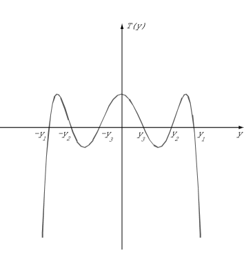
| (5.32) |
where the roots , and are related to the constants , and by the formulas
| (5.33) |
If all the roots are real, the behavior of the polynomial as a function of is shown on Fig. 1(a).
If all roots are distinct (), real periodic solutions are obtained for and . However, these are expressed in terms of elliptic functions and the period is not a multiple of . Constant solutions of eq. (5.32) are obviously , .
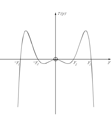
Elementary dependent real finite periodic solutions are obtained whenever the polynomial has multiple roots. The corresponding solutions are
(1) , (See Fig. 1(b))
| (5.34) |
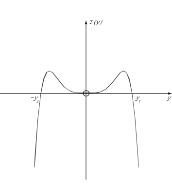
(2) (See Fig. 1(c))
| (5.35) |
or in terms of and :
| (5.36) |
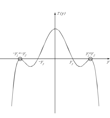
(3) (See Fig. 1(d))
In this case we give the solution implicitly as
| (5.37) |
The solution is real, finite and periodic for .
For any solution of eq. (5.31) we obtain a magnetic field and effective potential in the form
| (5.38) |
| (5.39) |
The functions , and figuring in the polar integral are
| (5.40) |
Let us sum up the results of this section. Three different cases of polar integrability exist. They are given by eq. (5.12), (5.22) to (5.24) and (5.38) to (5.40), respectively. The last case provides an example where the quantum system and the classical one differ. Indeed, the Planck constant figures explicitly in the effective potential and in the integral of motion.
6 Polar superintegrability
Let us assume that we have a Hamiltonian (1.1) that is “polar integrable”, i.e. allows an integral of motion of the form as in eq. (2.22). The magnetic field and effective potential must hence have one of the three forms established in Section 5. For the system to be superintegrable, it must allow at least one further integral, by assumption of the form (2.20). We can simplify this second integral by linear combinations with and with and also by rotations, since they will not destroy the form of (nor ). Thus, in eq. (2.20) we take , . Furthermore, we can assume , since otherwise we would be in the case of cartesian superintegrability, already treated in Section 4. By a rotation and normalization, we can set , . It follows that the second integral is of the parabolic type, conjugate to of eq. (2.23).
| (6.1) |
| (6.2) |
| (6.3) |
| (6.4) |
7 Conclusions
We have constructed all integrable quantum systems with a vector and scalar potential (as in eq. (1.1)) that possess either a first order integral, or a second order one of the cartesian, or polar type.
It is interesting to compare such systems with a nonzero magnetic field with systems allowing a scalar potential only.
1. The first difference is that for quantum and classical integrable systems with second order integrals do not necessarily coincide. The Planck constant can figure in a nontrivial way in the potentials and integrals of motion.
2. The existence of a first order integral of motion implies a geometrical symmetry, both for and . Indeed, a first order integral exists if and only if we have either , , or , (up to Euclidean transformations). The functions and are arbitrary in both cases.
3. The existence of a second order integral for implies that the Schrödinger equation will allow separation of variables in cartesian, polar, parabolic, or elliptic coordinates. In each case the potential depends on two arbitrary functions of one variable. For the coordinates no longer separate. The requirement that an irreducible second order integral should exist for is much more restrictive than for . The quanttities and again depend on two functions of one variable, however these functions obey certain ordinary differential equations. They are hence determined completely, up to some arbitrary constants. For instance, in the cartesian case, they are elliptic functions, or degenerate cases of elliptic functions.
4. For four families of superintegrable systems in exist [1], each depending on three parameters. For we have shown that superintegrability with first order integrals of the cartesian, or polar type, exists only for and constant.
Several related problems are presently under consideration. To complete the study of quadratic integrability in for we must still consider parabolic and elliptic integrability. For their is a close relation between superintegrability and exact solvability [20]. For the requirement of superintegrability seems to be too restrictive. An important question is whether some of the integrable systems found in this article are actually exactly solvable.
Acknowledgements
The research of P.W. was partly supported by research grants from NSERC of Canada and FQRNT du Québec.
References
- [1] I. Fris, V. Mandrosov, J. Smorodinsky, M. Uhlir, P. Winternitz, On higher symmetries in quantum mechanics, Phys. Lett. 16, 354-356 (1965).
- [2] P. Winternitz, J. Smorodinsky, M. Uhlir, I. Fris, Symmetry groups in classical and quantum mechanics, Sov. J. Nucl. Phys. 4, 444-450 (1967).
- [3] A. Makarov, J. Smorodinsky, Kh. Valiev, P. Winternitz, A systematic search for nonrelativistic systems with dynamical symmetries, Nuovo Cim. A 52, 1061-1084 (1967).
- [4] N.W. Evans, Superintegrability in classical mechanics, Phys. Rev. A 41, 5666-5676 (1990).
- [5] N.W. Evans, Group theory of the Smorondinsky-Winternitz system, J. Math. Phys. 32, 3369-3375 (1991).
- [6] E.G. Kalnins, G.C. Williams, W. Miller Jr, G.S. Pogosyan, Superintegrability in three-dimensional Euclidean space, J. Math. Phys. 40, 708-725 (1999).
- [7] E.G. Kalnins, J.M. Kress, G.S. Pogosyan, W. Miller Jr, Completeness of superintegrability in two-dimensional constant curvature spaces, J. Phys. A 34, 4705-4720 (2001).
- [8] E.G. Kalnins, J.M. Kress, W. Miller Jr and P. Winternitz, Superintegrable systems in Darboux spaces, J. Math. Phys, to appear.
- [9] S. Wojciechowski, Superintegrability of the Calogero-Moser system, Phys, Lett. A 95, 279-281 (1983).
- [10] M.A. Rodriguez, P. Winternitz, Quantum superintegrability and exact solvability in n dimensions, J. Math. Phys. 43, 3387-3410 (2002).
- [11] J. Hietarinta, Pure quantum integrability, Phys. Lett. A 246, 97-104 (1998).
- [12] J. Hietarinta, Classical vs quantum integrability, J. Math. Phys. 25, 1833-1840 (1984).
- [13] Gravel, S., Winternitz, P., Superintegrability with third-order integrals in quantum and classical mechanics, J. Math. Phys. 43, 5902-5912 (2002).
- [14] S. Gravel, Hamiltonians separable in cartesian coordinates and third-order integrals of motion Preprint arXiv math-ph/0302028, J. Math. Phys., to appear.
- [15] Dorizzi, B., Grammaticos, B., Ramani, A., Winternitz, P., Integrable Hamiltonian systems with velocity-dependent potentials, J. Math. Phys. 26, 3070-3079 (1985).
- [16] E. McSween, P. Winternitz, Integrable and superintegrable Hamiltonian systems in magnetic fields, J. Math. Phys. 41, 2957-2967 (2000).
- [17] M.B. Sheftel, P. Tempesta, P. Winternitz, Superintegrable systems in quantum mechanics and classical Lie theory, J. Math. Phys. 42, 659-673 (2001).
- [18] W. Miller Jr, Symmetry and separation of variables, Addison-Wesley, Reading, MA, 1977.
- [19] J. Bérubé, Systèmes intégrables et superintégrables classiques et quantiques avec champ magnétique, Mémoire, Université de Montréal, 2003.
- [20] P. Tempesta, A.V. Turbiner, P. Winternitz, Exact solvability of superintegrable systems, J. Math. Phys. 42, 4248-4257 (2001).