January 7, 2004

Segregation in the asymmetric Hubbard model

Abstract. We study the ‘asymmetric’ Hubbard model, where hoppings of electrons depend on their spin. For strong interactions and sufficiently asymmetric hoppings, it is proved that the ground state displays phase separation away from half-filling. This extends a recent result obtained with Freericks and Lieb for the Falicov-Kimball model. It is based on estimates for the sum of lowest eigenvalues of the discrete Laplacian in arbitrary domains.

Keywords: Hubbard model; Falicov-Kimball model; phase separation.

2000 Math. Subj. Class.: 82B10, 82B20, 82B26

Dedicated to Elliott Lieb on the occasion of his seventieth birthday.

1. Introduction

Electronic properties of condensed matter are difficult to apprehend because of the many-body interactions between quantum particles. It is necessary to consider simplified models that capture the physics of various systems. Of great relevance is the Hubbard model [13] where spin-$\frac{1}{2}$ electrons move on a lattice and interact via a local Coulomb repulsion. Although a considerable simplification to the original problem, the Hubbard model is still difficult to study and Hubbard himself considered an approximation where particles of one spin are infinitely massive and behave classically.

The latter model was reinvented later by Falicov and Kimball in a different context, namely in the study of the metal-semiconductor transition in rare-earth materials [5]. Two species of electrons corresponding to different electronic bands are moving on a lattice, and relevant interactions are between particles of different species. Electrons carry spins but these turn out to be mathematically irrelevant and they can be left aside. There exist many results for the Falicov-Kimball model. Let us mention proofs of long-range order [17, 1, 10, 15, 19, 25, 12] and of phase separation [16]; all these results are valid at half-filling, that is, the total density is equal to 1. Interfaces were studied in [4]. The ground state is segregated away from half-filling [6, 7]; see also [9]. There exist reviews by Gruber and Macris [11], Jȩdrzejewski and Lemański [14], and Freericks and Zlatić [8]. Less is known rigorously about the Hubbard model, see the survey by Lieb [22].

We consider here a Hamiltonian that interpolates between Hubbard and Falicov-Kimball and that describes two species of spinless fermions moving on ${\mathbb{Z}}^{d}$; particles have different effective masses, and there is a local interaction involving particles of different species. The Hamiltonian in second quantization is

$$H_{\Lambda}=-\sum_{\begin{subarray}{c}x,y\in\Lambda\\ |x-y|=1\end{subarray}}c_{x1}^{\dagger}c_{y1}-t\sum_{\begin{subarray}{c}x,y\in\Lambda\\ |x-y|=1\end{subarray}}c_{x2}^{\dagger}c_{y2}+U\sum_{x\in\Lambda}n_{x1}n_{x2}.$$ (1.1)

Here $\Lambda$ is a finite cube in ${\mathbb{Z}}^{d}$ and $c_{xj}^{\dagger}$ and $c_{xj}$ are creation and annihilation operators of a fermion of species $j$ at site $x$. The first two terms represent the kinetic energy of light and heavy electrons respectively (we suppose that $0\;\leqslant\;t\;\leqslant\;1$). $n_{xj}=c_{xj}^{\dagger}c_{xj}$ is a particle number operator. The positive parameter $U$ measures the strength of the on-site repulsion between particles of species 1 and 2.

Setting $t=1$ yields the Hubbard model, and $t=0$ yields the Falicov-Kimball model. It is interesting to note that the behavior of both models is similar when both particles have density $\frac{1}{2}$: for $d\;\geqslant\;2$, the ground state of the Hubbard model is a spin singlet [21], and the one of the Falicov-Kimball displays long-range order of the chessboard type [17]. This holds for all strictly positive values of the coupling constant $U$. It is natural to conjecture that long-range order occurs for all $t$.

Convergent perturbative expansions for large $U$ are a major source of results for the Falicov-Kimball model, at least at half-filling. See [3] and [18] for general methods, and [2] for a discussion specifically to the Falicov-Kimball model. These methods are robust and extend to any perturbation of the model. This holds in particular in the case of the asymmetric Hubbard model with small $t$.

Our goal is to identify a phase with with segregation and to contrast it with chessboard order and with high-temperature disorder. This suggests to look at the following operator,

$$\sigma_{\Lambda}(x)=\frac{1}{|\Lambda|}\sum_{y\in\Lambda}[n_{y2}-n_{y+x,2}]^{2}.$$ (1.2)

The corresponding correlation function is given by the expectation of $\sigma_{\Lambda}(x)$ in the equilibrium state. We consider here the canonical ensemble where densities of light and heavy particles are fixed to $\rho_{1}$ and $\rho_{2}$ respectively. High temperature states are translation invariant and exponentially clustering, and the correlation function converges to $2\rho_{2}(1-\rho_{2})$ as $x\to\infty$. Notice that $0<2\rho_{2}(1-\rho_{2})\;\leqslant\;\frac{1}{2}$. We identify here a domain of parameters where the expectation of $\sigma_{\Lambda}(x)$ is zero in the ground state (segregation). At half-filling perturbation methods [3, 18, 2] show that it is close to 1 when $|x|$ is odd (chessboard order).

Theorem 1.

Suppose that $\rho_{1}+\rho_{2}\neq 1$. There exist $U_{0}<\infty$ and $t_{0}>0$ (that depend on $\rho_{1}$ and $\rho_{2}$ only) such that for $U>U_{0}$ and $t<t_{0}$ we have

$$\bigl{(}\Upsilon_{\Lambda},\sigma_{\Lambda}(x)\Upsilon_{\Lambda}\bigr{)}=O(|\Lambda|^{-\frac{1}{d}}).$$

Here $\Upsilon_{\Lambda}$ is any ground state in the subspace where light and heavy particles have densities $\rho_{1}$ and $\rho_{2}$, respectively.

This theorem extends the result of [6, 7] for the Falicov-Kimball model. Its proof proceeds by obtaining estimates for the ground state energy. The ground state is a linear combination of states with a fixed configuration of heavy particles. The weight of configurations with large ‘boundary’ (pairs of nearest-neighbor sites where one is occupied and one is empty) is small. Indeed, most of light particles are delocalized in the remaining sites and their kinetic energy would otherwise be great, as it is roughly proportional to the boundary (see [6] and Section 2). The pressure exerted by the light particles packs the heavy particles together. The kinetic energy of heavy particles is therefore irrelevant, and simple estimates suffice in bounding their contribution. These ideas are detailed in Section 4.

Section 2 reviews the results for the sum of lowest eigenvalues of the discrete Laplacian obtained in [6], with some improvements in the regime of low densities. We discuss the segregated states of the asymmetric Hubbard model for all $0\;\leqslant\;t\;\leqslant\;1$ in Section 3. For given densities of light and heavy particles, there is one free parameter to characterize segregation: the proportion of volume occupied by each type of particles. The restricted phase diagram of segregate states displays a transition between a phase where the local density of heavy particles is maximum (that is, 1), and a phase where they have a local density that is strictly less than 1. Section 4 is devoted to the proof of Theorem 1.

Acknowledgements: I am grateful to both referees for useful comments, and to Lotfi Hermi for drawing my attention to the paper [24]. This paper is dedicated to Elliott Lieb on the occasion of his seventieth birthday. With Tom Kennedy, Elliott Lieb reinvented the Falicov-Kimball model and obtained the first rigorous results [17]. I enormously benefitted from a collaboration with him and Jim Freericks on segregation in this model; the present paper is directly inspired by [6].

2. Sum of lowest eigenvalues of the discrete Laplacian

The sum of the $N$ lowest eigenvalues of the discrete Laplacian in a finite domain $\Lambda\subset{\mathbb{Z}}^{d}$ gives the ground state energy of $N$ spinless, non-interacting electrons hopping in $\Lambda$. This quantity is relevant to some problems of condensed matter physics. Thermodynamics suggests that it is equal to a bulk term that is proportional to the volume $|\Lambda|$ of the domain, plus a positive boundary correction that is proportional to the boundary of $\Lambda$. Li and Yau proved in 1983 that the sum of lowest eigenvalues of the continuum Laplacian is indeed bounded below by the bulk term [20]. See [23], Theorem 12.3, for a clear exposition. The proof readily adapts to the case of the lattice.

The problem on the lattice turns out to be simpler and allows for bounds on the boundary correction, for given ‘electronic density’ $\rho=N/|\Lambda|$. Precisely, the boundary correction can be bounded above and below by positive numbers times the ‘surface’ of the boundary. This was done in [6]; this section contains some improvements in the limit of low densities.

Corresponding statements in the continuum case have not been obtained yet. The best statements seem to be the upper bound of Lieb and Loss, Theorem 12.11 in [23], and the lower bound of Melas [24], who obtained a positive correction of the order of the size of the domain to the power $d-2$. However, these bounds are not proportional to the boundary when the density is fixed.

For a finite domain $\Lambda\subset{\mathbb{Z}}^{d}$ the discrete Laplacian $h_{\Lambda}$ is defined by

$$h_{\Lambda}\varphi(x)=-\sum_{\begin{subarray}{c}y\in\Lambda\\ |y-x|=1\end{subarray}}\varphi(y)+2d\varphi(x),$$ (2.1)

for all $x\in\Lambda$. Here $\varphi\in\ell_{2}(\Lambda)$ is a normalized, complex function on $\Lambda$. If $\varphi$ is an eigenstate with eigenvalue $e$, so is $(-1)^{|x|}\varphi$ with eigenvalue $4d-e$ (here $|x|$ denotes the $\ell_{1}$ norm of $x\in{\mathbb{Z}}^{d}$). One also checks that $h_{\Lambda}\;\geqslant\;0$, and therefore its spectrum is contained in $(0,4d)$ and is symmetric around $2d$. The bulk term involves the ground state energy per site $e(\rho)$ of free fermions and it is given by

$$e(\rho)=\frac{1}{(2\pi)^{d}}\int_{\varepsilon_{k}<\varepsilon_{\rm F}(\rho)}\varepsilon_{k}\,{\rm d}k.$$ (2.2)

Here $k\in[-\pi,\pi]^{d}$ and $\varepsilon_{k}=2d-2\sum_{i=1}^{d}\cos k_{i}$. Notice that $|k|^{2}-\tfrac{1}{12}|k|^{4}\;\leqslant\;\varepsilon_{k}\;\leqslant\;|k|^{2}$. The ‘Fermi level’ $\varepsilon_{\rm F}(\rho)$ is defined by the equation

$$\rho=\frac{1}{(2\pi)^{d}}\int_{\varepsilon_{k}<\varepsilon_{\rm F}(\rho)}{\rm d}k.$$ (2.3)

Let $B(\Lambda)$ denote the number of bonds connecting $\Lambda$ with its complement,

$$B(\Lambda)=\bigl{|}\bigl{\{}(x,y):x\in\Lambda,y\in\Lambda^{\text{\rm c}},\text{ and }|x-y|=1\bigr{\}}\bigr{|}.$$ (2.4)

If $S_{\Lambda,N}$ is the sum of the $N$ lowest eigenvalues of $h_{\Lambda}$, and $\rho=N/|\Lambda|$ is the density, we are looking for bounds of the form

$$e(\rho)|\Lambda|+a(\rho)B(\Lambda)\;\leqslant\;S_{\Lambda,N}\;\leqslant\;e(\rho)|\Lambda|+b(\rho)B(\Lambda)$$ (2.5)

with positive $a(\rho)$, $b(\rho)$, that are independent of the domain. It was proved in [6] that

$$b(\rho)=\rho-\tfrac{1}{2d}e(\rho)$$ (2.6)

gives the optimal upper bound, that is saturated by domains consisting of isolated sites. (The size of the boundary was defined differently in [6] but minor changes in the proof yield the upper bound stated here.)

We define $a(\rho)$ to be the minimal ‘surface energy’ among all possible domains. Namely, for $\rho\in[0,1]\cap{\mathbb{Q}}$,

$$a(\rho)=\inf_{\Lambda}\,\frac{S_{\Lambda,N}-e(\rho)|\Lambda|}{B(\Lambda)}.$$ (2.7)

The infimum is taken over all finite domains $\Lambda$ such that $\rho|\Lambda|=N$ is an integer. The symmetry of the spectrum of $h_{\Lambda}$ around $2d$ implies that $a(1-\rho)=a(\rho)$. We give below lower and upper bounds, stating in particular that $a(\rho)>0$ for $0<\rho<1$. Many questions remain open, such as the existence of a minimizer in (2.7); continuity of $a(\rho)$; monotonicity and convexity of $a(\rho)$ for $0\;\leqslant\;\rho\;\leqslant\;\frac{1}{2}$. It is even not clear whether the infimum (2.7) can be taken on connected sets. In order to state the bounds for $a(\rho)$, let us introduce

$$\xi(\rho)=\rho\,\varepsilon_{\rm F}(\rho)-e(\rho).$$ (2.8)

Theorem 2.

For all $0<\rho\;\leqslant\;\frac{1}{2}$, we have

$$0<a(\rho)\;\leqslant\;\tfrac{1}{2d}\xi(\rho).$$

For small densities, we have

$$a(\rho)>\tfrac{2}{(3d)^{3}}\xi(\rho)\,\bigl{(}1-O(\rho^{2/d})\bigr{)}.$$

We prove here that $a(\rho)$ is bounded below by $\frac{2}{(3d)^{3}}\xi(\rho)$ at low densities and that it is smaller than $\frac{1}{2d}\xi(\rho)$; notice that $\xi(\rho)\sim\rho^{1+\frac{2}{d}}$ as $\rho\to 0$. Efforts are made here to get the best possible factor. On the other hand, pushing the range of densities instead, we could get a positive lower bound for $0<\rho<(4\pi)^{-d/2}\Gamma(\frac{d}{2}+1)^{-1}$. Remaining densities are much more difficult to treat and we refer to [6] (and to [9] for subsequent improvements and simplifications).

Proof of the lower bound for $a(\rho)$ for low densities..

We follow [6], with some improvements. Let $\varphi_{j}$ be the eigenvector of $h_{\Lambda}$ corresponding to the $j$-th eigenvalue $e_{j}$, and $\hat{\varphi}_{j}$ be its Fourier transform

$$\hat{\varphi}_{j}(k)=\sum_{x\in\Lambda}\varphi_{j}(x)\,{\rm e}^{{\rm i}kx}\,,\quad k\in[-\pi,\pi]^{d}.$$ (2.9)

Then

$$S_{\Lambda,N}=\frac{1}{(2\pi)^{d}}\int_{[-\pi,\pi]^{d}}{\boldsymbol{\rho}}(k)\,\varepsilon_{k}\,{\rm d}k,$$ (2.10)

where

$${\boldsymbol{\rho}}(k)=\sum_{j=1}^{N}|\hat{\varphi}_{j}(k)|^{2}=|\Lambda|-\sum_{j=N+1}^{|\Lambda|}|\hat{\varphi}_{j}(k)|^{2}.$$ (2.11)

We also observe that $\frac{1}{(2\pi)^{d}}\int{\boldsymbol{\rho}}(k){\rm d}k=N$. One obtains a lower bound for $S_{\Lambda,N}$ by taking the infimum of the right side of (2.10) over all positive functions ${\boldsymbol{\rho}}$ smaller than $|\Lambda|$ and with the proper normalization. This gives the bulk term [20, 23, 6]. In order to extract the effect of the boundary, one strengthens the upper bound for ${\boldsymbol{\rho}}(k)$, aiming at $|\Lambda|-{\text{\rm const}}\cdot B(\Lambda)$. We start as in [6] and write down a Schrödinger equation that is valid for all $x\in{\mathbb{Z}}^{d}$:

$$-\sum_{e}\varphi_{j}(x+e)+2d\varphi_{j}(x)+\raise 2.0pt\hbox{$\chi$}_{\Lambda^{\text{\rm c}}}(x)\sum_{e:x+e\in\Lambda}\varphi_{j}(x+e)=e_{j}\varphi_{j}(x).$$ (2.12)

It is understood that $\varphi_{j}(x)=0$ if $x\notin\Lambda$; the sums are over unit vectors $e$. The term with the characteristic function $\raise 2.0pt\hbox{$\chi$}_{\Lambda^{\text{\rm c}}}$ involves only sites that are close to the boundary. The Fourier transform of this equation can be written as

$$\varepsilon_{k}\hat{\varphi}_{j}(k)+(b_{k},\varphi_{j})=e_{j}\hat{\varphi}_{j}(k),$$ (2.13)

where $b_{k}$ is the following ‘boundary vector’

$$b_{k}(x)=\raise 2.0pt\hbox{$\chi$}_{\partial\Lambda}(x)\,{\rm e}^{-{\rm i}kx}\,\sum_{e:x+e\notin\Lambda}\,{\rm e}^{-{\rm i}ke}\,.$$ (2.14)

We introduced the set $\partial\Lambda$ of sites inside $\Lambda$ touching its complement

$$\partial\Lambda=\{x\in\Lambda:{\operatorname{dist\,}}(x,\Lambda^{\text{\rm c}})=1\}.$$ (2.15)

We observe that $B(\Lambda)\;\leqslant\;\|b_{k}\|^{2}\;\leqslant\;2dB(\Lambda)$, the lower bound holding at least when $|k|_{\infty}\;\leqslant\;\frac{\pi}{4}$. The last term of (2.11) can then be written using (2.13) as

$$\sum_{j=N+1}^{|\Lambda|}|\hat{\varphi}_{j}(k)|^{2}=\sum_{j=N+1}^{|\Lambda|}\frac{|(b_{k},\varphi_{j})|^{2}}{(e_{j}-\varepsilon_{k})^{2}}\;\geqslant\;\frac{\bigl{(}\sum_{j=N+1}^{|\Lambda|}|e_{j}-\varepsilon_{k}|\,|(b_{k},\varphi_{j})|^{2}\bigr{)}^{4}}{\bigl{(}\sum_{j=N+1}^{|\Lambda|}|e_{j}-\varepsilon_{k}|^{2}\,|(b_{k},\varphi_{j})|^{2}\bigr{)}^{3}}.$$ (2.16)

The lower bound follows from Hölder’s inequality. One easily checks that

$$\begin{split}&\sum_{j=N+1}^{|\Lambda|}|e_{j}-\varepsilon_{k}|\,|(b_{k},\varphi_{j})|^{2}\;\geqslant\;(b_{k},h_{\Lambda}b_{k})-(\varepsilon_{k}+e_{N})\|b_{k}\|^{2},\\ &\sum_{j=N+1}^{|\Lambda|}|e_{j}-\varepsilon_{k}|^{2}\,|(b_{k},\varphi_{j})|^{2}\;\leqslant\;(b_{k},h_{\Lambda}^{2}b_{k})+\varepsilon_{k}^{2}\,\|b_{k}\|^{2}.\end{split}$$ (2.17)

From now on we suppose $\varepsilon_{k}$ and $e_{N}$ to be small so that they add to less than 1. Notice that $(b_{k},h_{\Lambda}^{2}b_{k})=\|h_{\Lambda}b_{k}\|^{2}$. Because each site of $\partial\Lambda$ has a neighbor outside $\Lambda$ and $b_{k}$ is zero there, we have

$$(b_{k},h_{\Lambda}b_{k})=\sum_{\{x,y\}:|x-y|=1}\bigl{|}b_{k}(x)-b_{k}(y)\bigr{|}^{2}\;\geqslant\;\sum_{x\in\partial\Lambda}|b_{k}(x)|^{2}=\|b_{k}\|^{2}.$$ (2.18)

Then (2.16), (2.17), and (2.18), imply that

$$\sum_{j=N+1}^{|\Lambda|}|\hat{\varphi}_{j}(k)|^{2}\;\geqslant\;\frac{(b_{k},h_{\Lambda}b_{k})^{4}(1-\varepsilon_{k}-e_{N})^{4}}{(\|h_{\Lambda}b_{k}\|^{2}+\varepsilon_{k}^{2}\|b_{k}\|^{2})^{3}}.$$ (2.19)

We estimate the denominator.

$$\begin{split}\|h_{\Lambda}b_{k}\|^{2}&=\sum_{x\in\Lambda}\Bigl{|}\sum_{\begin{subarray}{c}y\in{\mathbb{Z}}^{d}\\ |y-x|=1\end{subarray}}\bigl{(}b_{k}(x)-b_{k}(y)\bigr{)}\Bigr{|}^{2}\\ &\;\leqslant\;2d\sum_{x\in\Lambda}\sum_{\begin{subarray}{c}y\in{\mathbb{Z}}^{d}\\ |y-x|=1\end{subarray}}\Bigl{|}b_{k}(x)-b_{k}(y)\Bigr{|}^{2}\\ &=2d\sum_{\begin{subarray}{c}x,y\in{\mathbb{Z}}^{d}\\ |x-y|=1\end{subarray}}\Bigl{|}b_{k}(x)-b_{k}(y)\Bigr{|}^{2}-2d\sum_{\begin{subarray}{c}x\in\Lambda^{\text{\rm c}},y\in\Lambda\\ |x-y|=1\end{subarray}}|b_{k}(y)|^{2}\\ &\;\leqslant\;4d(b_{k},h_{\Lambda}b_{k})-2d\|b_{k}\|^{2}.\end{split}$$ (2.20)

Inserting this bound in (2.19), we obtain

$$\sum_{j=N+1}^{|\Lambda|}|\hat{\varphi}_{j}(k)|^{2}\;\geqslant\;(1-\varepsilon_{k}-e_{N})^{4}\|b_{k}\|^{2}\frac{(b_{k},h_{\Lambda}b_{k})/\|b_{k}\|^{2}}{\bigl{[}4d-(2d-\varepsilon_{k}^{2})\frac{\|b_{k}\|^{2}}{(b_{k},h_{\Lambda}b_{k})}\bigr{]}^{3}}.$$ (2.21)

Simple analysis shows that the minimum of the fraction under the condition $(b_{k},h_{\Lambda}b_{k})\;\geqslant\;\|b_{k}\|^{2}$ is equal to $\frac{2}{(3d)^{3}}(1-\frac{\varepsilon_{k}^{2}}{2d})$. Furthermore, $b_{k}(x)$ is close to $b_{0}(x)$ for small $k$,

$$\begin{split}|b_{k}(x)|^{2}&=\Bigl{|}\sum_{e:x+e\notin\Lambda}(\cos ke-{\rm i}\sin ke)\Bigr{|}^{2}\;\geqslant\;\Bigl{|}\sum_{e:x+e\notin\Lambda}\cos ke\Bigr{|}^{2}\\ &\;\geqslant\;\Bigl{|}(1-\tfrac{1}{2}\varepsilon_{k})\sum_{e:x+e\notin\Lambda}1\Bigr{|}^{2}\;\geqslant\;(1-\varepsilon_{k})b_{0}^{2}(x).\end{split}$$ (2.22)

Clearly, $(1-\varepsilon_{k}-e_{N})^{4}(1-\frac{\varepsilon_{k}^{2}}{2d})(1-\varepsilon_{k})\;\geqslant\;1-6\varepsilon_{k}-4e_{N}$. Using (2.21) and (2.22) and since $\|b_{0}\|^{2}\;\geqslant\;B(\Lambda)$, we get

$$\sum_{j=N+1}^{|\Lambda|}|\hat{\varphi}_{j}(k)|^{2}\;\geqslant\;\tfrac{2}{(3d)^{3}}(1-6\varepsilon_{k}-4e_{N})B(\Lambda).$$ (2.23)

We can insert this estimate into (2.11) so as to get

$${\boldsymbol{\rho}}(k)\;\leqslant\;|\Lambda|-\tfrac{2}{(3d)^{3}}(1-6\varepsilon_{k}-4e_{N})B(\Lambda).$$ (2.24)

Suppose we have a bound ${\boldsymbol{\rho}}(k)\;\leqslant\;(1-\alpha)|\Lambda|$ for some $\alpha$ that is independent of $k$. Lieb and Loss ‘bathtub principle’ (Theorem 1.14 in [23]) yields

$$\begin{split}S_{\Lambda,N}&\;\geqslant\;(1-\alpha)|\Lambda|\frac{1}{(2\pi)^{d}}\int_{\varepsilon_{k}<\varepsilon_{\rm F}(\frac{\rho}{1-\alpha})}\varepsilon_{k}\,{\rm d}k\\ &=(1-\alpha)e(\tfrac{\rho}{1-\alpha})|\Lambda|.\end{split}$$ (2.25)

And because $(1-\alpha)e(\frac{\rho}{1-\alpha})$ is convex as a function of $\alpha$, and that its derivative is equal to $\xi(\frac{\rho}{1-\alpha})$, we obtain

$$S_{\Lambda,N}\;\geqslant\;e(\rho)|\Lambda|+\alpha\xi(\rho)|\Lambda|.$$ (2.26)

Let $0<\eta<1$. We define

$$\alpha=\tfrac{2}{(3d)^{3}}(1-\eta)\tfrac{B(\Lambda)}{|\Lambda|}.$$ (2.27)

The condition (2.24) implies that ${\boldsymbol{\rho}}(k)\;\leqslant\;(1-\alpha)|\Lambda|$ for all $k$ such that $\varepsilon_{k}<\varepsilon_{\rm F}(\frac{\rho}{1-\alpha})$, provided the following condition holds true,

$$\eta\;\geqslant\;6\varepsilon_{\rm F}(\tfrac{\rho}{1-\alpha})+4e_{N}.$$ (2.28)

Given $\eta$, we restrict to densities small enough so that

$$6\varepsilon_{\rm F}\bigl{(}\tfrac{\rho}{1-\frac{4}{27d^{2}}}\bigr{)}<\tfrac{1}{2}\eta.$$ (2.29)

(Notice that $\frac{4}{27d^{2}}$ is an upper bound for $\alpha$.) Then for all domains $\Lambda$ and all numbers of electrons $N$ such that $4e_{N}<\frac{1}{2}\eta$, the condition (2.28) is satisfied and we obtain

$$S_{\Lambda,N}\;\geqslant\;e(\rho)|\Lambda|+\tfrac{2}{(3d)^{3}}(1-\eta)\xi(\rho)B(\Lambda).$$ (2.30)

Consider now the case where (2.29) is fulfilled but $4e_{N}>\frac{1}{2}\eta$. We define $N^{\prime}$ such that $4e_{N^{\prime}}\;\leqslant\;\frac{1}{2}\eta$ and $4e_{N^{\prime}+1}>\frac{1}{2}\eta$. Then

$$\begin{split}S_{\Lambda,N}&=S_{\Lambda,N^{\prime}}+\sum_{j=N^{\prime}+1}^{N}e_{j}\\ &\;\geqslant\;e(\rho^{\prime})|\Lambda|+\tfrac{2}{(3d)^{3}}(1-\eta)\xi(\rho^{\prime})B(\Lambda)+\tfrac{1}{8}\eta(\rho-\rho^{\prime})|\Lambda|.\end{split}$$ (2.31)

The right side is larger than $e(\rho)|\Lambda|+\frac{2}{(3d)^{3}}(1-\eta)\xi(\rho)B(\Lambda)$ provided that

$$e(\rho^{\prime})+\tfrac{2}{(3d)^{3}}(1-\eta)\xi(\rho^{\prime})\tfrac{B(\Lambda)}{|\Lambda|}+\tfrac{1}{8}\eta(\rho-\rho^{\prime})\;\geqslant\;e(\rho)+\tfrac{2}{(3d)^{3}}(1-\eta)\xi(\rho)\tfrac{B(\Lambda)}{|\Lambda|}.$$ (2.32)

It is enough to check that the function $\frac{1}{8}\eta\rho-e(\rho)-\frac{4}{27d^{2}}\xi(\rho)$ is increasing. The derivative of $\xi(\rho)$ is equal to $\rho\frac{{\rm d}}{{\rm d}\rho}\varepsilon_{\rm F}(\rho)$. It is possible to verify that

$$\tfrac{{\rm d}}{{\rm d}\rho}\varepsilon_{\rm F}(\rho)<\tfrac{8\pi}{d}\Gamma(\tfrac{d}{2}+1)^{2/d}\rho^{-1+\frac{2}{d}}$$ (2.33)

(the bound is optimal in the limit $\rho\to 0$). The function above is therefore increasing for small densities. The number $\eta$ can be chosen arbitrarily small by taking the density small enough. Precisely, the condition is that ${\text{\rm const}}\cdot\rho^{2/d}\;\leqslant\;\eta$. This means that given $\rho$, we can take $\eta=O(\rho^{2/d})$. ∎

Proof of the upper bound for $a(\rho)$..

Let $\Lambda$ be a (rather large) domain, and $\Lambda^{\prime}$ be a set of isolated sites outside of $\Lambda$. Let $r$ be such that $|\Lambda^{\prime}|=r|\Lambda|$. The spectrum of $h_{\Lambda\cup\Lambda^{\prime}}$ is given by the union of the spectrum of $h_{\Lambda}$ and of $\{2d\}$, the latter eigenvalue being at least $|\Lambda^{\prime}|$ times degenerated. We have $S_{\Lambda,N}\;\geqslant\;S_{\Lambda\cup\Lambda^{\prime},N}$ (with equality if $\frac{N}{|\Lambda|}\;\leqslant\;\frac{1}{2}$) and $B(\Lambda^{\prime})=B(\Lambda)+2dr|\Lambda|$. Using the upper bound for $S_{\Lambda,N}$ and the lower bound for $S_{\Lambda\cup\Lambda^{\prime},N}$, we obtain (with $\rho=\frac{N}{|\Lambda|(1+r)}$)

$$e\bigl{(}(1+r)\rho\bigr{)}|\Lambda|+b\bigl{(}(1+r)\rho\bigr{)}B(\Lambda)\;\geqslant\;(1+r)e(\rho)|\Lambda|+a(\rho)\bigl{[}B(\Lambda)+2dr|\Lambda|\bigr{]}.$$ (2.34)

Reorganizing,

$$a(\rho)\Bigl{[}\frac{B(\Lambda)}{|\Lambda|}+2dr\Bigr{]}\;\leqslant\;e\bigl{(}(1+r)\rho\bigr{)}-(1+r)\,e(\rho)+b\bigl{(}(1+r)\rho\bigr{)}\frac{B(\Lambda)}{|\Lambda|}.$$ (2.35)

This inequality holds for any domain $\Lambda$ such that $(1+r)\rho|\Lambda|$ is an integer. Ratios boundary/volume can be made arbitrarily small and therefore the corresponding terms can be omitted. We obtain

$$a(\rho)\;\leqslant\;\frac{e\bigl{(}(1+r)\rho\bigr{)}-(1+r)\,e(\rho)}{2dr}.$$ (2.36)

Taking the limit $r\to 0$ yields the result. ∎

3. A discussion of segregation

Particles of different species segregate away from half-filling, at least for large $U$ and small $t$. The domain splits into two subdomains, $\Lambda=\Lambda_{1}\cup\Lambda_{2}$, with $\Lambda_{1}$ containing light particles only, and $\Lambda_{2}$ containing heavy particles only. This is true up to boundary terms that do not contribute to the bulk energy. We neglect boundary terms in this section.

There is one free parameter that controls segregation, namely the ratio of the volumes occupied by each phase. For $t=0$ the ground state is realized with $|\Lambda_{2}|=N_{2}$; it was argued in [6] that light particles exert a ‘pressure’ that packs heavy particles together; this pressure overcomes the tendency of heavy particles to delocalize so as to decrease their own kinetic energy. If $t$ is large enough however, heavy particles will extend their domain. We study this mechanism in this section, assuming that particles always segregate. From the point of view of rigorous results, we obtain upper bounds for the ground state energy of the system.

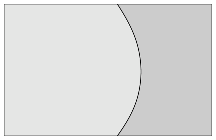
$\Lambda_{1}$$\frac{\rho_{1}}{1-\nu}$$\Lambda_{2}$$\frac{\rho_{2}}{\nu}$$\Lambda$

Figure 1. A segregated state involves a partition of the domain into subdomains $\Lambda_{1}$ and $\Lambda_{2}$ for light and heavy particles respectivey. The boundary between subdomains is supposed to be small so that its contribution to the bulk energy is negligible. With $\nu$ such that $|\Lambda_{2}|=\nu|\Lambda|$, densities inside each subdomain are $\frac{\rho_{1}}{1-\nu}$ and $\frac{\rho_{2}}{\nu}$.

We consider a finite domain $\Lambda\subset{\mathbb{Z}}^{d}$ partitioned in two subdomains $\Lambda_{1}$ and $\Lambda_{2}$. We fix the number of particles $N_{1}$ and $N_{2}$ of light and heavy particles respectively, and we denote the corresponding densities by $\rho_{1}=N_{1}/|\Lambda|$ and $\rho_{2}=N_{2}/|\Lambda|$. Let $\nu=|\Lambda_{2}|/|\Lambda|$; we have $\rho_{2}\;\leqslant\;\nu\;\leqslant\;1-\rho_{1}$. Notice that the densities inside each subdomain are $\frac{N_{1}}{|\Lambda_{1}|}=\frac{\rho_{1}}{1-\nu}$ and $\frac{N_{2}}{|\Lambda_{2}|}=\frac{\rho_{2}}{\nu}$. Neglecting the contribution of boundaries, the energy per site of this segregated state is

$$e(\rho_{1},\rho_{2};\nu)=(1-\nu)\,e(\tfrac{\rho_{1}}{1-\nu})+t\,\nu\,e(\tfrac{\rho_{2}}{\nu}).$$ (3.1)

For given densities $\rho_{1}$ and $\rho_{2}$ we are looking for the minimum of $e(\rho_{1},\rho_{2};\nu)$ with respect to $\nu$. One easily computes

$$\frac{{\rm d}}{{\rm d}\nu}e(\rho_{1},\rho_{2};\nu)=\xi(\tfrac{\rho_{1}}{1-\nu})-t\,\xi(\tfrac{\rho_{2}}{\nu}).$$ (3.2)

It is worth noticing that $e(\rho_{1},\rho_{2};\nu)$ is convex in $\nu$, as its second derivative is positive ($\xi$ is increasing). At $\nu=\rho_{2}$, we have

$$\frac{{\rm d}}{{\rm d}\nu}e(\rho_{1},\rho_{2};\nu)\Big{|}_{\nu=\rho_{2}}=\xi(\tfrac{\rho_{1}}{1-\rho_{2}})-2dt.$$ (3.3)

This expression can be positive or negative, the critical parameter being $t_{\rm c}=\frac{1}{2d}\xi(\frac{\rho_{1}}{1-\rho_{2}})$. On the other hand, the derivative of $e(\rho_{1},\rho_{2};\nu)$ at $\nu=1-\rho_{1}$ is always positive (if $t\;\leqslant\;1$). Therefore the segregated state that has minimum energy (among segregated states) is given as follows:

• If $t\;\leqslant\;t_{\rm c}=\frac{1}{2d}\xi(\frac{\rho_{1}}{1-\rho_{2}})$, the minimizer is $\nu=\rho_{2}$, and the phase of heavy particles has density 1.

• If $t_{\rm c}<t<1$, the minimizer $\nu$ is between $\rho_{2}$ and $\frac{\rho_{2}}{\rho_{1}+\rho_{2}}$, and the phase of heavy particles has a density strictly larger than $\rho_{1}+\rho_{2}$ and strictly smaller than 1.

• If $t=1$ the minimizer is $\nu=\frac{\rho_{2}}{\rho_{1}+\rho_{2}}$ and the phase of heavy particles has density $\rho_{1}+\rho_{2}$.

This is illustrated in Fig. 2, that displays a restricted phase diagram where only segregated states are considered. This description is relevant only if a segregated state minimizes the energy. This is proved in the case of small $t$.

A major open question in this model is whether segregation really occurs for $t>t_{\rm c}$.

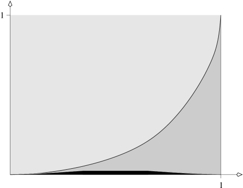
$t$$t_{\rm c}=\frac{1}{2d}\xi(\frac{\rho_{1}}{1-\rho_{2}})$$\frac{\rho_{1}}{1-\rho_{2}}$

Figure 2. Restricted phase diagram for segregated states. The phase of heavy particles has density 1 in the dark gray domain; its density is strictly less than 1 in the light gray domain. Segregation is proved in the black domain when $U=\infty$ (and in a smaller domain when $U$ is large).

4. The ground state of the asymmetric Hubbard model

Let ${\mathcal{F}}(\Lambda)$ be the Fock space for spinless fermions in $\Lambda$. For $\Lambda^{\prime}\subset\Lambda$, let $\Phi_{\Lambda^{\prime}}\in{\mathcal{F}}(\Lambda)$ represents the state with $|\Lambda^{\prime}|$ particles occupying all sites of $\Lambda^{\prime}$. $\{\Phi_{\Lambda^{\prime}}\}_{\Lambda^{\prime}\subset\Lambda}$ is a basis for ${\mathcal{F}}(\Lambda)$. The state space for the asymmetric Hubbard model is ${\mathcal{F}}(\Lambda)\otimes{\mathcal{F}}(\Lambda)$. Any function $\Upsilon_{\Lambda}\in{\mathcal{F}}(\Lambda)\otimes{\mathcal{F}}(\Lambda)$ can be written as

$$\Upsilon_{\Lambda}=\sum_{\Lambda_{1},\Lambda_{2}\subset\Lambda}a_{\Lambda_{1},\Lambda_{2}}\Phi_{\Lambda_{1}}\otimes\Phi_{\Lambda_{2}},$$ (4.1)

with $\sum_{\Lambda_{1},\Lambda_{2}}|a_{\Lambda_{1},\Lambda_{2}}|^{2}=1$. Let $a_{\Lambda_{2}}=(\sum_{\Lambda_{1}}|a_{\Lambda_{1},\Lambda_{2}}|^{2})^{1/2}$ and $\Psi(\Lambda_{2})\in{\mathcal{F}}(\Lambda)$ be the normalized function such that

$$a_{\Lambda_{2}}\Psi(\Lambda_{2})=\sum_{\Lambda_{1}\subset\Lambda}a_{\Lambda_{1},\Lambda_{2}}\Phi_{\Lambda_{1}}.$$ (4.2)

Then $\sum_{\Lambda_{2}}a_{\Lambda_{2}}^{2}=1$, and the function $\Upsilon_{\Lambda}$ can be written as

$$\Upsilon_{\Lambda}=\sum_{\Lambda_{2}\subset\Lambda}a_{\Lambda_{2}}\Psi(\Lambda_{2})\otimes\Phi_{\Lambda_{2}}.$$ (4.3)

We derive in Proposition 3 below an inequality for the coefficients $a_{\Lambda_{2}}$ that will allow us to establish segregation in the ground state of the strongly asymmetric Hubbard model.

Let ${\mathcal{F}}(\Lambda;N)$ denote the Hilbert subspace of ${\mathcal{F}}(\Lambda)$ corresponding to $N$ particles. That is, it is spanned by $\{\Phi_{\Lambda^{\prime}}\}$ with $|\Lambda^{\prime}|=N$. All spaces ${\mathcal{F}}(\Lambda;N_{1})\otimes{\mathcal{F}}(\Lambda;N_{2})$ are invariant under the action of $H_{\Lambda}$ since the latter conserves both particle numbers. As before, we denote densities by $\rho_{1}=\frac{N_{1}}{|\Lambda|}$ and $\rho_{2}=\frac{N_{2}}{|\Lambda|}$. The term $\gamma(U)$ that appears below was defined in [6]; it behaves like $\frac{8d^{2}}{U}$ for large $U$.

Proposition 3.

Let $\Upsilon_{\Lambda}$ be a ground state of $H_{\Lambda}$ in ${\mathcal{F}}(\Lambda;N_{1})\otimes{\mathcal{F}}(\Lambda;N_{2})$. If $a(\frac{\rho_{1}}{1-\rho_{2}})>\gamma(U)+t$, we have

$$\sum_{\Lambda_{2}\subset\Lambda}a_{\Lambda_{2}}^{2}B(\Lambda_{2})\;\leqslant\;\frac{4d\,b(\frac{\rho_{1}}{1-\rho_{2}})\rho_{2}^{1-\frac{1}{d}}}{a(\frac{\rho_{1}}{1-\rho_{2}})-\gamma(U)-t}\;|\Lambda|^{1-\frac{1}{d}}.$$

Proof.

We write the energy of a state using coefficients $a_{\Lambda_{2}}$ defined above, and then use results obtained for the Falicov-Kimball model. Let $T_{\Lambda}$ be the kinetic energy operator for particles in $\Lambda$; it acts on ${\mathcal{F}}(\Lambda)$, and can be written as

$$T_{\Lambda}=-\sum_{\begin{subarray}{c}x,y\in\Lambda\\ |x-y|=1\end{subarray}}c_{x}^{\dagger}c_{y}$$ (4.4)

where $c_{x}^{\dagger}$ and $c_{x}$ are creation and annihilation operators of a fermion at x. Notice that the kinetic terms of (1.1) are given by $T_{\Lambda}\otimes{\mathchoice{\rm 1\mskip-4.0mul}{\rm 1\mskip-4.0mul}{\rm 1\mskip-4.5mul}{\rm 1\mskip-5.0mul}}+t{\mathchoice{\rm 1\mskip-4.0mul}{\rm 1\mskip-4.0mul}{\rm 1\mskip-4.5mul}{\rm 1\mskip-5.0mul}}\otimes T_{\Lambda}$. Furthermore, for $\Lambda^{\prime}\subset\Lambda$, let $V_{\Lambda,\Lambda^{\prime}}$ be the operator

$$V_{\Lambda,\Lambda^{\prime}}=U\sum_{x\in\Lambda^{\prime}}c_{x}^{\dagger}c_{x}.$$ (4.5)

It represents an external potential that is equal to $U$ on sites of $\Lambda^{\prime}$ and 0 otherwise. The energy of a state $\Upsilon_{\Lambda}$ given by (4.3) can be written as

$$(\Upsilon_{\Lambda},H_{\Lambda}\Upsilon_{\Lambda})=t\sum_{\Lambda_{2},\Lambda_{2}^{\prime}}a_{\Lambda_{2}}a_{\Lambda_{2}^{\prime}}(\Psi(\Lambda_{2}),\Psi(\Lambda_{2}^{\prime}))\,(\Phi_{\Lambda_{2}},T_{\Lambda}\Phi_{\Lambda_{2}^{\prime}})\\ +\sum_{\Lambda_{2}}a_{\Lambda_{2}}^{2}\bigl{(}\Psi(\Lambda_{2}),(T_{\Lambda}+V_{\Lambda,\Lambda_{2}})\Psi(\Lambda_{2})\bigr{)}.$$ (4.6)

(The sums are over sets satisfying $|\Lambda_{2}|=|\Lambda_{2}^{\prime}|=N_{2}$.) Notice that the first term of the right side is bounded by

$$t\sum_{\Lambda_{2},\Lambda_{2}^{\prime}}{}^{\prime}a_{\Lambda_{2}}a_{\Lambda_{2}^{\prime}}\;\leqslant\;t\Bigl{(}\sum_{\Lambda_{2},\Lambda_{2}^{\prime}}{}^{\prime}a_{\Lambda_{2}}^{2}\Bigr{)}^{1/2}\Bigl{(}\sum_{\Lambda_{2},\Lambda_{2}^{\prime}}{}^{\prime}a_{\Lambda_{2}^{\prime}}^{2}\Bigr{)}^{1/2}=t\sum_{\Lambda_{2}}a_{\Lambda_{2}}^{2}B(\Lambda_{2}),$$ (4.7)

where the symbol $\sum{}^{\prime}$ means a sum over pairs of sets $\Lambda_{2},\Lambda_{2}^{\prime}\subset\Lambda$ that differ only by one site moved to a neigbor (that is, the symmetric difference $\Lambda_{2}\triangle\Lambda_{2}^{\prime}$ must be a pair of nearest-neigbors).

The strategy of the proof is to consider the expression (4.6) for the energy of the ground state $\Upsilon_{\Lambda}$. We get an upper bound by using a trial function that is independent of the coefficients $\{a_{\Lambda_{2}}\}$. We then estimate the second term of (4.6) from below, using the inequality (2.5) for the segregation energy. The corresponding expression involves the coefficients $\{a_{\Lambda_{2}}\}$ and we obtain the inequality stated in Proposition 3.

Let $\Lambda_{2}\subset\Lambda$ be such that $|\Lambda_{2}|=N_{2}$, and let us consider $\Psi(\Lambda_{2})\otimes\Phi_{\Lambda_{2}}$ where $\Psi(\Lambda_{2})$ is a normalized function of ${\mathcal{F}}(\Lambda,N_{1})$ with support on $\Lambda_{2}^{\text{\rm c}}$. We have

$$(\Psi(\Lambda_{2})\otimes\Phi_{\Lambda_{2}},H_{\Lambda}\,\Psi(\Lambda_{2})\otimes\Phi_{\Lambda_{2}}) =(\Psi(\Lambda_{2}),T_{\Lambda_{2}^{\text{\rm c}}}\Psi(\Lambda_{2}))$$

$$\;\leqslant\;|\Lambda_{2}^{\text{\rm c}}|e(\tfrac{\rho_{1}}{1-\rho_{2}})+b(\tfrac{\rho_{1}}{1-\rho_{2}})B(\Lambda_{2}).$$ (4.8)

We used the upper bound in (2.5). We take for $\Lambda_{2}$ a square if possible, or a domain with very close shape. Its boundary is less than $4dN_{2}^{1-\frac{1}{d}}$. The boundary term in (4.8) is then smaller than $4d\,b(\tfrac{\rho_{1}}{1-\rho_{2}})\rho_{2}^{1-\frac{1}{d}}|\Lambda|^{1-\frac{1}{d}}$. We use now the lower bound in (2.5). As stated in this paper it holds only for $U=\infty$. However, it was extended in [6] to finite $U$; namely, it was shown there that

$$\bigl{(}\Psi(\Lambda_{2}),(T_{\Lambda}+V_{\Lambda})\Psi(\Lambda_{2})\bigr{)}\;\geqslant\;e(\tfrac{\rho_{1}}{1-\rho_{2}})|\Lambda_{2}^{\text{\rm c}}|+[a(\tfrac{\rho_{1}}{1-\rho_{2}})-\gamma(U)]B(\Lambda_{2}),$$ (4.9)

where $a(\cdot)$ is the minimal surface energy defined in (2.7). Combining this with (4.6) and (4.7), we have for any ground state function $\Upsilon_{\Lambda}$,

$$(\Upsilon_{\Lambda},H_{\Lambda}\Upsilon_{\Lambda})\;\geqslant\;-t\sum_{\Lambda_{2}}a_{\Lambda_{2}}^{2}B(\Lambda_{2})+\sum_{\Lambda_{2}}a_{\Lambda_{2}}^{2}\Bigl{[}e(\tfrac{\rho_{1}}{1-\rho_{2}})|\Lambda_{2}^{\text{\rm c}}|+\bigl{(}a(\tfrac{\rho_{1}}{1-\rho_{2}})-\gamma(U)\bigr{)}B(\Lambda_{2})\Bigr{]}.$$ (4.10)

We now compare this expression with the upper bound (4.8) and we obtain

$$\sum_{\Lambda_{2}}a_{\Lambda_{2}}^{2}B(\Lambda_{2})\Bigl{[}a(\tfrac{\rho_{1}}{1-\rho_{2}})-\gamma(U)-t\Bigr{]}\;\leqslant\;4d\,b(\tfrac{\rho_{1}}{1-\rho_{2}})\rho_{2}^{1-\frac{1}{d}}|\Lambda|^{1-\frac{1}{d}}.$$ (4.11)

∎

Proof of Theorem 1.

Using the decomposition (4.3) for the ground state $\Upsilon_{\Lambda}$, we have

$$(\Upsilon_{\Lambda},\sigma_{\Lambda}(x)\Upsilon_{\Lambda})=\frac{2}{|\Lambda|}\sum_{y\in\Lambda}\sum_{\Lambda_{2}\subset\Lambda}a_{\Lambda_{2}}^{2}\raise 2.0pt\hbox{$\chi$}_{\Lambda_{2}}(y)\,\raise 2.0pt\hbox{$\chi$}_{\Lambda_{2}^{\text{\rm c}}}(x+y).$$ (4.12)

It is clear that

$$\sum_{y\in\Lambda}\raise 2.0pt\hbox{$\chi$}_{\Lambda_{2}}(y)\,\raise 2.0pt\hbox{$\chi$}_{\Lambda_{2}^{\text{\rm c}}}(x+y)\;\leqslant\;B(\Lambda_{2})\,|x|_{\infty},$$ (4.13)

and therefore

$$(\Upsilon_{\Lambda},\sigma_{\Lambda}(x)\Upsilon_{\Lambda})\;\leqslant\;\frac{2|x|_{\infty}}{|\Lambda|}\sum_{\Lambda_{2}\subset\Lambda}a_{\Lambda_{2}}^{2}B(\Lambda_{2}).$$ (4.14)

Hole-particle symmetries in this model are similar to those in the Falicov-Kimball model, see [17], and allow to restrict to the case $\rho_{1}+\rho_{2}<1$. We have $a(\frac{\rho_{1}}{1-\rho_{2}})>\gamma(U)+t$ if $U$ is large and $t$ is small, so that Proposition 3 is valid. We use it to control the sum above and we get Theorem 1. ∎

References

• [1] U. Brandt and R. Schmidt, Exact results for the distribution of the f-level ground state occupation in the spinless Falicov-Kimball model, Z. Phys. B 63, 45–53 (1986)
• [2] N. Datta, R. Fernández, and J. Fröhlich, Effective Hamiltonians and phase diagrams for tight-binding models, J. Stat. Phys. 96, 545–611 (1999)
• [3] N. Datta, R. Fernández, J. Fröhlich, and L. Rey-Bellet, Low-temperature phase diagrams of quantum lattice systems. II. Convergent perturbation expansion ans stability in systems with infinite degeneracy, Helv. Phys. Acta 69, 752–820 (1996)
• [4] N. Datta, A. Messager, and B. Nachtergaele, Rigidity of interfaces in the Falicov-Kimball model, J. Stat. Phys. 99, 461–555 (2000)
• [5] L. M. Falicov and J. C. Kimball, Simple model for semiconductor-metal transitions: SmB6 and transition-metal oxides, Phys. Rev. Lett. 22, 997–9 (1969)
• [6] J. K. Freericks, E. H. Lieb, and D. Ueltschi, Segregation in the Falicov-Kimball model, Commun. Math. Phys. 227, 243–79 (2002)
• [7] J. K. Freericks, E. H. Lieb, and D. Ueltschi, Phase separation due to quantum mechanical correlations, Phys. Rev. Lett. 88, 106401 (2002)
• [8] J. K. Freericks and V. Zlatić, Exact dynamical mean-field theory of the Falicov-Kimball model, Rev. Mod. Phys. 75, 1333–82 (2003)
• [9] P. Goldbaum, Lower bound for the segregation energy in the Falicov-Kimball model, Physica A 36, 2227–34 (2003)
• [10] Ch. Gruber, J. Jȩdrzejewski, and P. Lemberger, Ground states of the spinless Falicov-Kimball model II, J. Stat. Phys. 66, 913–38 (1992)
• [11] Ch. Gruber and N. Macris, The Falicov-Kimball model: a review of exact results and extensions, Helv. Phys. Acta 69, 850–907 (1996)
• [12] K. Haller and T. Kennedy, Periodic ground states in the neutral Falicov-Kimball model in two dimensions, J. Stat. Phys. 102, 15–34 (2001)
• [13] J. Hubbard, Electron correlations in narrow energy bands, Proc. Roy. Soc. London A 276, 238–57 (1963)
• [14] J. Jȩdrzejewski and R. Lemański, Falicov-Kimball models of collective phenomena in solids (a concise guide), Acta Phys. Pol. B 32, 3243–52 (2001)
• [15] T. Kennedy, Some rigorous results on the ground states of the Falicov-Kimball model, Rev. Math. Phys. 6, 901–25 (1994)
• [16] T. Kennedy, Phase separation in the neutral Falicov-Kimball model, J. Stat. Phys. 91, 829–43 (1998)
• [17] T. Kennedy and E. H. Lieb, An itinerant electron model with crystalline or magnetic long range order, Physica A 138, 320–58 (1986)
• [18] R. Kotecký and D. Ueltschi, Effective interactions due to quantum fluctuations, Commun. Math. Phys. 206, 289–335 (1999)
• [19] J. L. Lebowitz and N. Macris, Long range order in the Falicov-Kimball model: extension of Kennedy-Lieb theorem, Rev. Math. Phys. 6, 927–46 (1994)
• [20] P. Li and S.-T. Yau, On the Schrödinger equation and the eigenvalue problem, Commun. Math. Phys. 88, 309–18 (1983)
• [21] E. H. Lieb, Two theorems on the Hubbard model, Phys. Rev. Lett. 62, 1201–4; Errata 62, 1927 (1989)
• [22] E. H. Lieb, The Hubbard model: some rigorous results and open problems, XIth International Congress of Mathematical Physics (Paris, 1994), 392–412, Internat. Press (1995)
• [23] E. H. Lieb and M. Loss, Analysis, 2nd edition, Amer. Math. Soc. (2001)
• [24] A. D. Melas, A lower bound for sums of eigenvalues of the Laplacian, Proc. Amer. Math. Soc. 131, 631–6 (2002)
• [25] A. Messager and S. Miracle-Solé, Low temperature states in the Falicov-Kimball model, Rev. Math. Phys. 8, 271–99 (1996)