Abstract

We introduce new modified Abelian lattice models, with inhomogeneous local interactions, in which a sum over topological sectors are included in the defining partition function. The dual models, on lattices with arbitrary topology, are constructed and they are found to contain sums over topological sectors, with modified groups, as in the original model. The role of the sum over sectors is illuminated by deriving the field-strength formulation of the models in an explicitly gauge-invariant manner. The field-strengths are found to satisfy, in addition to the usual local Bianchi constraints, global constraints. We demonstrate that the sum over sectors removes these global constraints and consequently softens the quantization condition on the global charges in the system. Duality is also used to construct mappings between the order and disorder variables in the theory and its dual. A consequence of the duality transformation is that correlators which wrap around non-trivial cycles of the lattice vanish identically. For particular dimensions this mapping allows an explicit expression for arbitrary correlators to be obtained.

Keywords: Duality, Lattice, Topology, Statistical Models.

PACS Codes: 11.15.Ha, 11.15.-q, 12.40.Ee.

1 Introduction

In recent years various dualities have played an important role in identifying the non-perturbative objects in string theories and a web of connections between the perturbative string theories has been conjectured. Strong-Weak duality ($S$-duality) has also shed light on the strong coupling limit of $N=2$ supersymmetric gauge theories [2, 3]. However, the notion of duality has existed in statistical models since the early work of Kramers and Wannier [4] on the two dimensional Ising model. In their pioneering work duality was used to compute the critical temperature at which the Ising model undergoes a second order phase transition. $S$-duality has also been studied in the other spin models [5] and in the context of gauge theories on the lattice [6]. Recently, duality in generalized statistical models were studied on topologically non-trivial manifolds [7] and a method for constructing self-dual models was given. For other relevant work see [8, 9].

The lattice models considered here have degrees of freedom which take values in an Abelian group, ${\cal G}$, and live on the $(k-1)$-cells of the lattice with local interactions. These are generalizations of well known statistical models such as spin models and gauge theories. On topologically non-trivial manifolds there are configurations of the fields which have global charges around the non-trivial $k$-cycles of the lattice. For example, on a torus spin models can have vortex configurations which contains non-trivial flux around the two canonical cycles of the lattice. Analogously, the statistical sum of a gauge theory on $S^{2}\times S^{2}$ includes monopole configurations which have non-trivial charge around the two two-sphere’s. In the flat case the vortices, or monopoles etc., must satisfy certain quantization conditions (which depends on ${\cal G}$) around the elementary plaquettes , cubes, etc. . On topologically non-trivial manifolds the global charges must also be quantized. In [7] the global charges were forced to satisfy either the same quantization conditions as the local charges, or were completely free of quantization. In the present work we will not make such a restriction. This is implemented by introducing a sum over, what we will term, topological sectors of the theory over a subgroup of ${\cal G}$ (rather than the entire group, ${\cal G}$, or only its identity element, as in [7]). As a note, summing over these sectors is somewhat akin to introducing a sum over sectors in (super) Yang-Mills to obtain the correct $2\pi$-periodicity which was implemented in [10] (see also [11, 12]).

We will demonstrate that even in these models the duality transformations can be performed on arbitrary lattices. The topological sectors are found to appear in the dual model, however, the groups over which one sums over are modified through certain duality relations which we will derive. To understand the role that the sum over sectors play on the physical quantities in the model we rewrite the model in terms of the more natural field-strength variables [13, 14]. This rewriting shows that the sum over topological sectors relaxes the quantization conditions on the global charges which appear around the various $k$-cycles of the lattice. This allows the introduction of fractional global charges into the system. Using this new freedom we construct several self-dual models which are qualitatively distinct from earlier examples in that these models contain different fractional global charges around the various $k$-cycles of the lattice. In addition, as a consequence of duality we will prove that correlators which wrap around a non-trivial $(k-1)$-cycle of the lattice vanish identically. It is also demonstrated that if the dimension of the lattice and dimension of the cells on which the interactions take place are equal, then correlators are completely determined by the duality transformations. A particular example is that one can compute an arbitrary Wilson loop on a two-dimensional Riemann surface of a gauge theory, with the topological modifications, directly from duality. Due to the existence of a global fractional charge we find that the correlators are invariant under what one denotes by the inside and outside of a Wilson loop only if the representation of the loop respects the $n$-ality of the fractional charge. Similar results will hold for the higher-dimensional analogs.

The outline of the paper is as follows. In section 2 we introduce some notations and the language of simplicial homology required to define the models in their most natural form. The duality transformations are then carried out on the general model. To close the section several explicit examples of the models using standard notation are given and their duals are constructed. In the next section we rewrite the model in terms of the field-strengths, dynamical variables which live on cells of one higher dimension than the original degrees of freedom. This is performed in an explicitly gauge invariant manner. Such a rewriting leads to an understanding of what the sum over topological sectors imply physically. We will demonstrate that the sum relaxes the quantization conditions on the global charges in the system and can be used to introduce fractional charges around the various $k$-cycles of the lattice. Section 4 explores several examples of self-dual models which contain these fractional charges. Section 5 is a detailed discussion of order and disorder correlators, how duality relates them to one another, a proof that certain correlators vanish identically due to topological constraints, and an explicit computation of correlators in dimensions $d=k$. Finally in section 6 we make our concluding remarks. Throughout this work spin models and gauge theories are used in writing down explicit examples, however, it should be noted that it is straightforward to extend the examples to include higher dimensional fields.

2 The General Model and its Dual

It is possible to treat spin systems, gauge theories, anti-symmetric tensor field theories and all higher dimensional analogs, under a universal framework. This can be achieved if one restricts the Boltzmann weights to have local interactions only. By local interactions we mean the following: In a spin model the spins interact with their nearest neighbours, and the Boltzmann weights are link valued objects with arguments depending only the spins on the ends of the link. For a gauge theory the dynamical fields live on the links of the lattice, while the Boltzmann weight is a plaquette valued object and depends on the product of the fields around the plaquette. Anti-symmetric tensor field theories are restricted in a similar manner, the Boltzmann weights are defined on the elementary cubes of the lattice and depend on the product of the plaquettes around that cube. etc. In continuum language these models with local interactions are field theories in which the dynamical variable is a $(k-1)$-form, $\omega$, and the action depends solely on the exterior derivative of that form, ${\rm d}\omega$. This definition is taken even on manifolds with non-trivial topology. On the lattice, the statement that the interactions are local amount to insisting that the Boltzmann weights depends on the coboundary, $\delta\sigma$, of a $(k-1)$-chain, $\sigma$. This is the language of simplicial homology and a precise definition of the coboundary operator will be given shortly. To be self-contained and to introduce our notations we give a short review of this language in the next subsection.

2.1 Mathematical Preliminaries

We now give a short review of simplicial homology (for more details see e.g. [15]). Consider a lattice $\Omega$ and associate to every $k$-dimensional cell of the lattice an oriented generator $c_{k}^{(i)}$ where $i$ indexes the various cells of dimension $k$. These objects generate the $k$-chain group, denoted by $C_{k}(\Omega,{\cal G})$,

$$\sum_{i=1}^{{\cal N}_{k}}~{}g_{i}~{}c_{k}^{(i)}=g\in C_{k}(\Omega,{\cal G})\qquad,\qquad g_{i}\in{\cal G}$$

Here ${\cal G}$ is an arbitrary Abelian group with group multiplication implemented through addition and ${\cal N}_{k}$ is the number of $k$-cells in the lattice $\Omega$. An element $g\in C_{k}(\Omega,{\cal G})$ is called a ${\cal G}$-valued $k$-chain or simply a $k$-chain. Clearly $C_{k}(\Omega,{\cal G})=\oplus_{i=1}^{{\cal N}_{k}}{\cal G}$.

Two homomorphisms, the boundary $\partial$ and the coboundary $\delta$, define the chain complexes $(C_{*}(\Omega,{\cal G}),\partial)$ and $(C_{*}(\Omega,{\cal G}),\delta)$ where $C_{*}(\Omega,{\cal G})\equiv\oplus_{k=0}^{d}C_{k}(\Omega,{\cal G})$:

$$0\!\stackrel{{\scriptstyle\partial_{d+1}}}{{\longrightarrow}}\!C_{d}(\Omega,{\cal G})\!\stackrel{{\scriptstyle\partial_{d}}}{{\longrightarrow}}\!\dots\!\stackrel{{\scriptstyle\partial_{k+2}}}{{\longrightarrow}}\!C_{k+1}(\Omega,{\cal G})\!\stackrel{{\scriptstyle\partial_{k+1}}}{{\longrightarrow}}\!C_{k}(\Omega,{\cal G})\!\stackrel{{\scriptstyle\partial_{k}}}{{\longrightarrow}}\!C_{k-1}(\Omega,{\cal G})\!\stackrel{{\scriptstyle\partial_{k-1}}}{{\longrightarrow}}\!\dots C_{0}(\Omega,{\cal G})\!\stackrel{{\scriptstyle\partial_{0}}}{{\longrightarrow}}\!0$$

$$0\!\stackrel{{\scriptstyle\delta_{d}}}{{\longleftarrow}}\!C_{d}(\Omega,{\cal G})\!\stackrel{{\scriptstyle\delta_{d-1}}}{{\longleftarrow}}\!\dots\!\stackrel{{\scriptstyle\delta_{k+1}}}{{\longleftarrow}}\!C_{k+1}(\Omega,{\cal G})\!\stackrel{{\scriptstyle\delta_{k}}}{{\longleftarrow}}\!C_{k}(\Omega,{\cal G})\!\stackrel{{\scriptstyle\delta_{k-1}}}{{\longleftarrow}}\!C_{k-1}(\Omega,{\cal G})\!\stackrel{{\scriptstyle\delta_{k-2}}}{{\longleftarrow}}\dots C_{0}(\Omega,{\cal G})\!\stackrel{{\scriptstyle\delta_{-1}}}{{\longleftarrow}}\!0$$

These homomorphisms are defined by their actions on the generators $c_{k}^{(i)}$ (we display the dimension subscripts on $\partial_{k}$ and $\delta_{k}$ only when essential),

$$\partial c_{k}^{(i)}=\sum_{j=1}^{{\cal N}_{k-1}}[c_{k}^{(i)}:c_{k-1}^{(j)}]~{}c_{k-1}^{(j)}~{}~{},~{}~{}\delta c_{k}^{(i)}=\sum_{j=1}^{{\cal N}_{k+1}}[c_{k+1}^{(j)}:c_{k}^{(i)}]~{}c_{k+1}^{(j)}$$ (2.1)

where the incidence number is given by,

$$[c_{k}^{(i)}:c_{k-1}^{(j)}]=\left\{\begin{array}[]{ll}\pm 1&\mbox{if the $j^{{\rm th}}$ $(k-1)$-cell is contained in the $i^{{\rm th}}$ $k$-cell}\\ 0&\mbox{otherwise}\end{array}\right.$$

The plus or minus sign reflects the relative orientation of the cells. The boundary (coboundary) chains and the exact (coexact) chains are defined as,

$$\begin{array}[]{lclclcl}B_{k}(\Omega,{\cal G})&=&{\rm Im}~{}\partial_{k+1}&,&B^{k}(\Omega,{\cal G})&=&{\rm Im}~{}\delta_{k-1}\cr Z_{k}(\Omega,{\cal G})&=&{\rm ker}~{}\partial_{k}&,&Z^{k}(\Omega,{\cal G})&=&{\rm ker}~{}\delta_{k}\end{array}$$

These sets inherit their group structure from the chain complex. The boundary and coboundary operators are nilpotent: $\partial\partial=0$ and $\delta\delta=0$. The quotient groups,

$$H_{k}(\Omega,{\cal G})=Z_{k}(\Omega,{\cal G})/B_{k}(\Omega,{\cal G})\qquad,\qquad H^{k}(\Omega,{\cal G})=Z^{k}(\Omega,{\cal G})/B^{k}(\Omega,{\cal G})$$

are the homology and cohomology groups respectively. The elements of the homology group are those chains that have zero boundary and are themselves not the boundary of a higher dimensional chain, while the elements of the cohomology group are those chains that have zero coboundary and are themselves not the coboundary of a lower dimensional chain. In section 2.4 we will give some explicit examples for the 2-tori.

We define the projection of a chain onto cell via the following “inner product”,

$$\langle c_{k}^{(i)},c_{l}^{(j)}\rangle=\delta_{k,l}\;\delta^{i,j}$$

which is linear in both arguments. The boundary and coboundary operators are dual to each other with respect to this operation,

$$\langle\partial c_{k}^{(i)},c_{k-1}^{(j)}\rangle=\langle c_{k}^{(i)},\delta c_{k-1}^{(j)}\rangle$$ (2.2)

If $\Omega$ is a triangulation of an orientable manifold, then there exists the following set of isomorphisms between the homology and cohomology groups,

$$H_{k}(\Omega,Z\!\!\!Z)\cong H^{d-k}(\Omega,Z\!\!\!Z)\cong H^{k}(\Omega,Z\!\!\!Z)\cong H_{d-k}(\Omega,Z\!\!\!Z)$$ (2.3)

We will denote the generators of the homology group by $\{h_{a}:a=1,\dots,A_{k}\}$ and the cohomology group by $\{h^{a}:a=1,\dots,A^{k}\}$. The isomorphisms, (2.3), imply the following orthogonality relations for the generators,

$$\langle h_{a},h^{b}\rangle=\delta_{a}^{b}$$ (2.4)

and $h_{a}$ is said to be dual to $h^{a}$, not to be confused with interpreting on the dual lattice (to be defined shortly). The isomorphisms also imply that $A_{k}=A^{d-k}=A^{k}=A_{d-k}$.

Let us work out a few illustrative examples of how this language is used. Let $\sigma\in C_{0}(\Omega,{\cal G})$, consider the following inner product,

$$\langle\delta\sigma,c_{1}^{(l)}\rangle=\langle\sigma,\partial c_{1}^{(l)}\rangle=\langle\sum_{i=1}^{{\cal N}_{0}}\sigma_{i}\,c_{0}^{(i)},(c_{0}^{(l_{1})}-c_{0}^{(l_{2})})\rangle=\sum_{i=1}^{{\cal N}_{0}}\sigma_{i}\,\langle c_{0}^{(i)},(c_{0}^{(l_{1})}-c_{0}^{(l_{2})})\rangle=\sigma_{l_{1}}-\sigma_{l_{2}}$$

where the link $l$ points from the site $l_{1}$ to the site $l_{2}$. This is precisely the form of the interaction for a nearest neighbour spin model. As another example take $\sigma\in C_{1}(\Omega,{\cal G})$ and repeat the above,

$$\langle\delta\sigma,c_{2}^{(p)}\rangle=\langle\sigma,\partial c_{2}^{(p)}\rangle=\langle\sum_{l=1}^{{\cal N}_{1}}\sigma_{l}\,c_{1}^{(l)},\sum_{l^{\prime}\in p}c_{1}^{(l^{\prime})}\rangle=\sum_{l=1}^{{\cal N}_{1}}\sigma_{l}\,\sum_{l^{\prime}\in p}\langle c_{1}^{(l)},c_{1}^{(l^{\prime})}\rangle=\sum_{l^{\prime}\in p}\sigma_{l}$$

where $p$ labels the plaquette, and we have assumed that the links are oriented consistently with that plaquette so that no relative signs appear. Not surprisingly this reproduces the form of the Wilson-like terms in a lattice gauge theory.

It will be necessary at some point during the analysis in the next few sections to introduce the notion of the dual lattice. To obtain the dual lattice one introduces a new chain group generated by a new set of generators which are constructed from the generators of $C_{*}(\Omega,{\cal G})$. A generator of $C_{*}(\Omega^{*},{\cal G})$, $c_{k}^{*(i)}$, is obtained from the generators of $C_{*}(\Omega,{\cal G})$, $c_{k}^{(i)}$, by making the following identifications:

$$c_{k}^{(i)} \leftrightarrow c_{d-k}^{*(l)}$$ (2.5)

$$~{}[c_{k}^{(i)}:c_{k-1}^{(j)}] \leftrightarrow [c_{d-k+1}^{*(j)}:c_{d-k}^{*(i)}]$$ (2.6)

In general this identification does not produce a lattice, however in case the original lattice was a triangulation of a closed orientable manifold it does and these are the cases we study here. Under this identification one also finds that,

$$\langle\delta g,c_{k}^{(i)}\rangle \leftrightarrow \langle\partial g^{*},c_{d-k}^{*(i)}\rangle$$

$$\langle\partial g,c_{k-2}^{(i)}\rangle \leftrightarrow \langle\delta g^{*},c_{d-k+2}^{*(i)}\rangle$$ (2.7)

where $C_{k-1}(\Omega,{\cal G})\in g=\sum_{i=1}^{{\cal N}_{k-1}}g_{i}\;c_{k-1}^{(i)}$ and $C_{d-k+1}(\Omega^{*},{\cal G})\in g^{*}=\sum_{i=1}^{{\cal N}_{k-1}}g_{i}\;c_{d-k+1}^{*(i)}=\sum_{i-1}^{{\cal N}^{*}_{d-k+1}}g_{i}^{*}\;c_{d-k+1}^{*(i)}$. Consequently, the homology (cohomology) generators on the lattice $\Omega$ become cohomology (homology) generators on the dual lattice $\Omega^{*}$.

2.2 The Modified Abelian Lattice Theories

Now that the terminology is fixed the models can be introduced in their most general form. Consider an orientable lattice which has freely generated $k$-th cohomology group: $H^{k}(\Omega,Z\!\!\!Z)\cong Z\!\!\!Z\oplus\dots\oplus Z\!\!\!Z$, and let $\{h^{a}:a=1,\dots,A^{k}\}$ denote its generators. The model is defined through the following partition function,

$$Z=\sum_{\{n_{a}\in{\cal H}_{a}\}}\;\sum_{\sigma\in C_{k-1}(\Omega,{\cal G})}\;\prod_{p=1}^{{\cal N}_{k}}\;B_{p}\left(\left\langle\left(\delta\sigma+n_{a}h^{a}\right),c_{k}^{(p)}\right\rangle\right)$$ (2.8)

The groups ${\cal H}_{a}$ are in general subgroups of ${\cal G}$, and one must define the addition in the Boltzmann weights to mean addition in the group ${\cal G}$. For example, if ${\cal G}=U(1)$ and ${\cal H}_{a}=Z\!\!\!Z_{N}$ the addition should be written as $\delta\sigma~{}+~{}(2\pi/N)n_{a}h^{a}$. In the case ${\cal G}$ and/or ${\cal H}$ are continuous the sums should be replaced by the appropriate integrals. These models correspond to standard statistical models when ${\cal H}_{a}$ are taken to be identity elements in ${\cal G}$. For example, if $k=1$, (2.8) is a spin model with ${\cal G}$-valued spins on the sites of a lattice interacting with their nearest neighbour. For $k=2$, (2.8) is a gauge theory with gauge group ${\cal G}$ and Boltzmann weight having arguments which depend on the sum (since group multiplication is implemented additively here) of the links that make up a plaquette. When $k=3$ the model consists of an anti-symmetric tensor field where the arguments of the Boltzmann weights depend on the sum over plaquettes in an elementary cube. The role of the extra summations over $\{n_{a}\}$, which we will term topological sectors of theory, will be explained in section 3 once the model is written in terms of field-strength variables. It should be pointed out that some particular choices of the groups $\{{\cal H}_{a}\}$ reduces to the cases studied in [7] and [16] and will be elaborated on in section 2.4.

2.3 The Dual Model

In this section we will perform the duality transformations on (2.8). Although the method is fairly standard it is useful to demonstrate how it is carried out in this language. The first step is as always to introduce a character expansion for the Boltzmann weights,

$$B(g)=\frac{1}{|{\cal G}|}\sum_{r\in{\cal G}^{*}}b(r)\chi_{r}(g),\qquad b(r)=\sum_{g\in{\cal G}}\;B(g)\;\chi_{r}(g)$$ (2.9)

where $|{\cal G}|$ is the order of the group and ${\cal G}^{*}$ denotes the group of irreducible representations of ${\cal G}$, and inherits ${\cal G}$’s Abelian structure (for example ${\rm l\!R}^{*}={\rm l\!R}$, $U(1)^{*}=Z\!\!\!Z$, $Z\!\!\!Z_{N}^{*}=Z\!\!\!Z_{N}$). In the case ${\cal G}$, or ${\cal G}^{*}$, are continuous groups the normalized sum over group elements should be replaced by the appropriate integral. Throughout the remainder of this paper we will ignore overall constants to avoid clutter in the equations. The character expansion can be thought of as a Fourier transformation which respects the group symmetries. It is interesting to note that the set of irreducible representations of ${\cal G}$ form a group if and only if ${\cal G}$ is Abelian. This is the reason why it is difficult to derive duality relations for non-Abelian statistical models and field theories.

Due to the Abelian nature of the group, and its representations, the characters satisfy the following factorization properties,

$$\chi_{r}(g)\chi_{s}(g)=\chi_{r+s}(g)\quad,\quad\chi_{r}(g)\chi_{r}(g^{\prime})=\chi_{r}(g+g^{\prime})$$ (2.10)

In addition they satisfy the following orthogonality relations,

$$\sum_{g\in{\cal G}}\chi_{r}(g){\overline{\chi}}_{s}(g) = \delta_{{\cal G}^{*}}(r-s)$$

$$\sum_{r\in{\cal G}^{*}}\chi_{r}(g){\overline{\chi}}_{r}(g^{\prime}) = \delta_{{\cal G}}(g-g^{\prime})$$ (2.11)

where ${\overline{\chi}}_{s}(g)$ is the character of $g$ in the representation conjugate to $s$, i.e. $\chi_{-s}(g)$, and the subscript on the delta-function indicates that it is invariant under that group.

On inserting the character expansion (2.9) into the partition function, (2.8) the sum over representations and product over $k$-cells can be re-ordered. This introduces a representation, $r_{p}$, on every $k$-cell of the lattice, these representations can be encoded into a $k$-chain denoted by $r\equiv\sum_{p=1}^{{\cal N}_{k}}r_{p}c_{k}^{(p)}$. The partition function then becomes,

$$Z=\sum_{r\in C_{k}(\Omega,{\cal G}^{*})}\prod_{p=1}^{{\cal N}_{k}}b_{p}(\langle r,c_{k}^{(p)}\rangle)\sum_{\{n_{a}\in{\cal H}_{a}\}}\;\sum_{\sigma\in C_{k-1}(\Omega,{\cal G})}\;\prod_{p=1}^{{\cal N}_{k}}\;\chi_{\langle r,c_{k}^{(p)}\rangle}\left(\left\langle\left(\delta\sigma+n_{a}h^{a}\right),c_{k}^{(p)}\right\rangle\right)$$ (2.12)

Using the factorization properties of the characters, (2.10), and the definition of the (co)-boundary operator, (2.1), one can rewrite the product over characters in (2.12),

$$\prod_{p=1}^{{\cal N}_{k}}\chi_{\langle r,c_{k}^{(p)}\rangle}\left(\left\langle\left(\delta\sigma+n_{a}h^{a}\right),c_{k}^{(p)}\right\rangle\right)=\prod_{l=1}^{{\cal N}_{k-1}}\chi_{\langle\partial r,c_{k-1}^{(l)}\rangle}\left(\langle\sigma,c_{k-1}^{(l)}\rangle\right)\;\prod_{a=1}^{A^{k}}\chi_{\langle r,h^{a}\rangle}\left(n_{a}\right)$$ (2.13)

In the above the generators of the cohomology group were written as $h^{a}=\sum_{p\in\gamma^{a}}c_{k}^{(p)}$. The sum over $\sigma$ and $\{n_{a}\}$ in (2.12) can then be performed with use of the orthogonality relations, (2.11),

$$\sum_{\{n_{a}\in{\cal H}_{a}\}}\sum_{\sigma}\dots = \prod_{l=1}^{{\cal N}_{k-1}}\sum_{\sigma_{l}\in{\cal G}}\chi_{\langle\partial r,c_{k-1}^{(l)}\rangle}\left(\sigma_{l}\right)\;\prod_{a=1}^{A^{k}}\sum_{n_{a}\in{\cal H}_{a}}\chi_{\langle r,h^{a}\rangle}\left(n_{a}\right)$$ (2.14)

$$= \prod_{l=1}^{{\cal N}_{k-1}}\delta_{{\cal G}^{*}}\left(\langle\partial r,c_{k-1}^{(l)}\rangle\right)\;\prod_{a=1}^{A^{k}}\delta_{{\cal H}_{a}^{*}}\left(\langle r,h^{a}\rangle\right)$$

The first constraint implies that the boundary of the $k$-chain $r$ vanishes identically. The most general chain which satisfies that constraint is the sum of a boundary of a higher dimensional chain and an element of the $k$-th homology both carrying ${\cal G}^{*}$ coefficients:

$$r=\partial r^{\prime}+h,\quad{\rm where},\qquad r^{\prime}\in C_{k+1}(\Omega,{\cal G}^{*}),\quad h\in H_{k}(\Omega,{\cal G}^{*})$$ (2.15)

We will write the homology part of $r$ in terms of the generators of the homology group, $h=\sum_{a=1}^{A_{k}}{\widetilde{n}}_{a}h_{a}$. On inserting (2.15) into the remaining constraints in (2.14) and using the orthogonality (2.4) one finds that coefficients of the homology are further constrained,

$$\prod_{a=1}^{A_{k}}\delta_{{\cal H}_{a}^{*}}\left({\widetilde{n}}^{a}\right)$$ (2.16)

Since $\{{\widetilde{n}}^{a}\}$ are elements of ${\cal G}^{*}$ this constraint forces ${\widetilde{n}}^{a}\in{\cal G}^{*}\perp{\cal H}^{*}_{a}$ (those elements in $G^{*}$ which are the identity in $H^{*}$) where ${\widetilde{n}}_{a}$ is the coefficient of $h_{a}$ dual to $h^{a}$. Inserting (2.15) and (2.16) into the partition function (2.12) we obtain,

$$Z=\sum_{\{{\widetilde{n}}^{a}\in{\cal G}^{*}\perp{\cal H}_{a}^{*}\}}\;\sum_{r\in C_{k+1}(\Omega,{\cal G}^{*})}\;\prod_{p=1}^{{\cal N}_{k}}b_{p}\left(\left\langle\partial r+{\widetilde{n}}^{a}h_{a},c_{k}^{(p)}\right\rangle\right)$$ (2.17)

where the dummy prime index on $r^{\prime}$ from (2.15) has been removed. This representation of the model is not of the same form as original one since the argument of the Boltzmann weight contains a boundary operator acting on $r$ rather than a coboundary operator and since $\{{\widetilde{n}}^{a}\}$ are coefficients of homology rather than cohomology. However, if one interprets the objects on the dual lattice (see discussion at end of section 2.1) the partition function reads,

$$Z=\sum_{\{{\widetilde{n}}_{a}\in{\cal G}^{*}\perp{\cal H}_{a}^{*}\}}\;\sum_{r\in C_{d-k-1}(\Omega^{*},{\cal G}^{*})}\;\prod_{p=1}^{{\cal N}^{*}_{d-k}}b_{p}\left(\left\langle\delta r+{\widetilde{n}}_{a}h^{*a},c_{d-k}^{*(p)}\right\rangle\right)$$ (2.18)

Here $\{h^{*a}:a=1,\dots,A^{d-k}\}$ are the generators of $H^{d-k}(\Omega^{*},Z\!\!\!Z)$ which are obtained by considering the generators of $H_{k}(\Omega,Z\!\!\!Z)$ on the dual lattice. Notice that this final form of the dual theory has precisely the same form as the original model (2.8). Clearly the following criteria are necessary conditions for the model to be self-dual: the lattice must be self-dual, $k$ must be equal to $d-k$ so that the dynamical degrees of freedom are on the same types of cells and the coefficient group ${\cal G}$ must be isomorphic to its group of representations ${\cal G}^{*}$. Additional constraints on obtaining self-dual models are imposed by the cohomology coefficients $\{{\cal H}_{a}\}$. The set of ${\cal H}_{a}$ must reproduce itself under duality, consequently every group appearing in $\{{\cal H}_{a}\}$ must appear in $\{{\cal G}^{*}\perp{\cal H}_{a}^{*}\}$ with the same multiplicity. In the next sub-section we will demonstrate how to obtain some explicitly self-dual models using our results interpreted in standard language.

2.4 Illustrative Examples

Figure 1: Obtaining the dual theory to a spin model on surface of genus $g$ with a sum over $Z\!\!\!Z_{2}$ included over the cocycle in the first diagram. See text for details.

As mentioned earlier these models are generalizations of the models considered in [7, 16]. Here we will make the connection explicit and also introduce some examples which are unique to the present discussion. Let us deal in particular with the case $k=1$, ${\cal G}=Z\!\!\!Z_{2}$ and $\Omega$ is a square lattice triangulation of a $2$-tori. Since the dynamical variables live on the $(k-1)=0$-dimensional cells of the lattice and interact through a nearest neighbour coupling this corresponds to the Ising model with appropriate choice of Boltzmann weights. The relevant cohomology here is $H^{1}(\Omega,Z\!\!\!Z_{2})\cong Z\!\!\!Z_{2}\oplus Z\!\!\!Z_{2}\oplus Z\!\!\!Z_{2}\oplus Z\!\!\!Z_{2}$. To understand what the generators of this group are it is best to consider the homology group of dimension $d-k=1$ on the dual lattice. The generators of that group are well known: $h_{a}=\sum_{l\in\gamma^{*}_{a}}c_{1}^{(l)}$ where $\gamma^{*}_{a}$ are the set of links which wrap around the $a$-th handle of the 2-tori. The cohomology generators of dimensions $k=1$ are then obtained by interpreting each $\gamma^{*}_{a}$ back on the original lattice, denote that set of links by $\gamma_{a}$. One visualization of $\gamma_{a}$ are to view of them as “steps of a ladder” wrapping around the $a$-th handle of the 2-tori. This construction is quite general: if the lattice is orientable, first construct the generators of $H_{d-k}$ on the dual lattice, and then interpret back on the original lattice that will yield the generators of $H^{k}$. We will consider the model in which ${\cal H}_{1}=Z\!\!\!Z_{2}$ and all the rest are the identity element. The set of links $\gamma_{1}$ are depicted in the first diagram of Figure 1 by the solid lines forming steps around the handle. The model (2.8) in standard language is then given by,

$$Z=\sum_{n_{1}=\pm 1}\;\sum_{\{\sigma_{i}\}=\pm 1}\;\prod_{\langle ij\rangle\in\Omega}\;\exp\left\{(n_{1})^{\varepsilon({\gamma}_{1};ij)}\;\beta\;\sigma_{i}\sigma_{j}\right\}$$ (2.19)

here $i$ labels sites on the lattice, $\langle ij\rangle$ are nearest neighbours forming a link and,

$$\varepsilon({\gamma}_{1};ij)=\langle\gamma_{1},c_{1}^{(\langle ij\rangle)}\rangle=\langle\sum_{l\in\gamma_{1}}c_{1}^{(l)},c_{1}^{(\langle ij\rangle)}\rangle=\left\{\begin{array}[]{ll}1&\mbox{ if $\langle ij\rangle$ is in ${\gamma}_{1}$}\\ 0&\mbox{otherwise}\end{array}\right.$$ (2.20)

This model can be viewed as the sum of two Ising models: one which has coupling constant $\beta$ on every link and another with coupling $\beta$ on all links except for those contained in ${\gamma}_{1}$ where it is taken to be $-\beta$. Another view is to take the Ising model on a $2$-tori and slice the lattice along one canonical cycle on the dual lattice and then sew the lattice back together with the two possible “twists” in the coupling.

Let us now demonstrate how the dual model is obtained. The first step is to find the homology cycle which is dual, in the sense of (2.3), to the generator $h^{1}=\sum_{l\in{\gamma}_{1}}c_{1}^{(l)}$. The dual cycle, $h_{1}$, is depicted by the dotted line in the fist diagram in Figure 1. According to the analysis in the previous sub-section the coefficient group of $h_{1}$, in the dual theory before interpretation on the dual lattice (2.17), is ${\cal G}\perp{\cal H}=Z\!\!\!Z_{2}\perp Z\!\!\!Z_{2}=\{e\}$. Consequently, it is not summed over in the dual theory. The remaining cycles, depicted in the second diagram in Figure 1, have weight ${\cal G}\perp\{e\}=Z\!\!\!Z_{2}\perp\{e\}=Z\!\!\!Z_{2}$ and are summed over in the dual theory although they were absent in the original model. The final step is to interpret the groups associated with the cycles $h_{1},\dots,h_{4}$, as groups for the cocycles on the dual lattice ( see the third diagram in Figure 1). Denote these cocycles by $h_{1}^{*},h_{2}^{*},h_{3}^{*}$ (notice that $h_{1}^{*}$ is isomorphic to $h_{1}$, it is simply shifted by $\frac{1}{2}$ lattice spacing in both directions). The dual theory is then given by,

$$Z=c\left(\beta^{*}\right)\left(\prod_{a=1}^{3}\sum_{{\widetilde{n}}_{a}=\pm 1}\right)\;\sum_{\{\sigma_{i}^{*}\}=\pm 1}\;\prod_{\langle i,j\rangle\in\Omega^{*}}\;\exp\left\{\left(\prod_{a=1}^{3}(n_{a})^{\varepsilon(\gamma^{*a};ij)}\right)\;\beta^{*}\;\sigma^{*}_{i}\sigma^{*}_{j}\right\}$$ (2.21)

where $\beta^{*}=-\frac{1}{2}\ln\tanh\beta$ is the well known dual coupling constant and the overall non-singular piece $c(\beta^{*})=(2\sinh(2\beta^{*}))^{-\frac{{\cal N}_{1}}{2}}$ appears when performing the character expansion of the Boltzmann weight. Also, $\gamma^{*a}$ denotes the set of links which define $h^{*a}$. This particular example is clearly not self-dual. However, it is not difficult to convince oneself that if a sum over two cocycles, each in a separate handle, was included in the original model, then the dual model would be identical to the original one. Thus on the $2$-tori there are $4$ inequivalent self-dual theories: $\{1,3\}$,$\{1,4\}$,$\{2,3\}$ and $\{2,4\}$ where $\{i,j\}$ is intended to mean that a sum over the cocycle labeled by $i$ and $j$ was included (we order the cocycles so that 1 and 2 are around the first handle and 3 and 4 are around the second). There are of course more self-dual models formed by summing models of type (2.8). For example, a trivial way to obtain a self-dual model is to take a model, which is not self-dual, and add it to its dual (one could also subtract it from its dual to obtain anti-self-dual models). This however, does not exhaust all possible self-dual models that one can write down with ${\cal H}_{a}=Z\!\!\!Z_{2}$ or the identity. It is possible to find all of them by constructing a vector of partition functions where the index labels all possible partition functions, then carry out the duality transformation on each component of the vector, to obtain a new vector of partition functions. Each element of this “dual” vector must be a linear combination of the original vector of partition functions since it contained all possible partition functions. Consequently, one can construct a matrix which acts on the original vector to give to the dual vector. This matrix is a matrix representation of the duality transformation, and its eigenvectors with eigenvalues plus one (it could have eigenvalues minus one as well, since only its square must be the identity) label the possible self-dual models. An example of this was given in [7] and we will not repeat this construction here.

The Ising model example only considered the degenerate case of ${\cal H}_{a}={\cal G}$ or the identity. It is, however, possible to relax this condition and still obtain self-dual theories. Consider the case of a spin model on a $2$-dimensional Riemann surface and choose ${\cal G}={\rm l\!R}$ and $\{{\cal H}_{a}=2\pi RZ\!\!\!Z\}$. Since the coefficient group is identical for all cocycles, the dual theory is obtained by simply replacing ${\cal G}$ by ${\cal G}^{*}={\cal G}={\rm l\!R}$ and $\{{\cal H}_{a}\}$ by $\{{\cal G}^{*}\perp{\cal H}_{a}^{*}=R^{-1}Z\!\!\!Z\}$. This case was studied in [16] in the context of string theory on a circle, the change in the coefficient $2\pi R\to R^{-1}$ is a manifestation of target space duality (T-duality). Other examples with ${\cal H}_{a}={\cal H}\neq{\cal G}$ were studied in [16] in the context of string theory on discrete target spaces.

One further example of a self-dual spin-model on a Riemann surface is furnished by the case ${\cal G}=Z\!\!\!Z_{NM}$ and ${\cal H}_{i(a)}=Z\!\!\!Z_{N}$ and ${\cal H}_{i(b)}=Z\!\!\!Z_{M}$ where $(a)$ indicates an $a$-cycle (the short non-trivial cycle) and $(b)$ a $b$-cycle (the long non-trivial cycle) on the surface, and $i$ labels the handles. We will delay a description of this case until section 2.4 where they will be interpreted as fractionally charged models with different fractional charges around the various cycles of the lattice.

3 Local and Global Bianchi Identities

In pure gauge theories the action depends on the gauge fields only through their field-strengths. It seems more natural then to rewrite the theory so that the field-strengths are the dynamical degrees of freedom. Various authors [13, 14, 17] have shown that the price of doing this is the appearance of Bianchi constraints on the field-strengths. On the lattice the gauge fields live on links, while their field-strengths are defined on the plaquettes of the lattice. The Bianchi constraints are realized, in this situation, by forcing the group product of the field-strength variables in every elementary cube to be the identity element. In this section we consider the generalized problem where the models are defined by the partition function in (2.8) and we introduce a $k$-chain in place of the coboundary of the $(k-1)$-chain $\sigma$. Consequently, the results of 3.1 generalize the Abelian results found in [13, 14]. The variables which live on the $k$-dimensional cells will collectively be referred to as field-strengths. We will show that the partition function can be written in terms of field-strengths on topologically non-trivial lattices. The usual Bianchi identities that arise in the flat case are supplemented by constraints along the homology cycles of the lattice as a direct consequence of the duality transformations derived in the previous section. This will be demonstrated in an explicitly gauge-invariant manner. The role of the sum over topological sectors will also be illuminated by this rewriting of the model.

3.1 Computation of The Constraints

It is possible to write down the natural choice of constraints by counting degrees of freedom [17] which are introduced in the field-strength formulation, however, we would like to derive them explicitly. To do so, we make use of a Fadeev-Popov trick by inserting the following identity into the partition function (2.8),

$$1=\sum_{f\in C_{k}(\Omega,{\cal G})}\;\delta_{{\cal G}}\left(f-(\delta\sigma+n_{a}h^{a})\right)$$

On insertion into (2.8) and re-ordering the summations one finds,

$$Z=\sum_{f\in C_{k}(\Omega,{\cal G})}\;\prod_{p=1}^{{\cal N}_{k}}\;B_{p}\left(\left\langle f,c_{k}^{(p)}\right\rangle\right)\Pi(f)$$ (3.1)

where $\Pi(f)$ is the constraint sum,

$$\Pi(f)\equiv\sum_{\{n_{a}\in{\cal H}_{a}\}}\;\sum_{\sigma\in C_{k-1}(\Omega,{\cal G})}\;\prod_{p=1}^{{\cal N}_{k}}\delta_{{\cal G}}\left(\left\langle(f-(\delta\sigma+n_{a}h^{a}),c_{k}^{(p)}\right\rangle\right)$$

Notice that $\Pi(f)$ is itself a partition function of the form (2.8) where the Boltzmann weights are ${\cal G}$-invariant delta functions, the presence of the chain $f$ can be interpreted as an external field acting on the system. The character coefficients of such a Boltzmann weight are obviously,

$$b_{p}(r)={\overline{\chi}}_{r}(\langle f,c_{k}^{(p)}\rangle)$$

The dual representation of $\Pi(v)$, before interpretation on the dual lattice, is straightforward to write down and is given by (2.17),

$$\Pi(f) = \sum_{\{{\widetilde{n}}^{a}\in{\cal G}^{*}\perp{\cal H}_{a}^{*}\}}\;\sum_{r\in C_{k+1}(\Omega,{\cal G}^{*})}\;\prod_{p=1}^{{\cal N}_{k}}{\overline{\chi}}_{\langle\partial r+{\widetilde{n}}^{a}h_{a},c_{k}^{(p)}\rangle}\left(\langle f,c_{k}^{(p)}\rangle\right)$$

$$= \left[\sum_{r\in C_{k+1}(\Omega,{\cal G}^{*})}\;\prod_{p=1}^{{\cal N}_{k}}{\overline{\chi}}_{\langle\partial r,c_{k}^{(p)}\rangle}\left(\langle f,c_{k}^{(p)}\rangle\right)\right]\!\!\left[\sum_{\{{\widetilde{n}}^{a}\in{\cal G}^{*}\perp{\cal H}_{a}^{*}\}}\prod_{p=1}^{{\cal N}_{k}}{\overline{\chi}}_{\langle{\widetilde{n}}^{a}h_{a},c_{k}^{(p)}\rangle}\left(\langle f,c_{k}^{(p)}\rangle\right)\right]$$

$$\equiv \Pi_{1}(f)\;\Pi_{2}(f)$$

The factorization properties (2.10) was used to obtain the second equality. This form of the constraints demonstrate that they are two distinct classes of constraints: a topologically trivial term $\Pi_{1}(f)$ and a term which is purely topological $\Pi_{2}(f)$. We will treat these two sectors separately. Using (2.13), $\Pi_{1}(f)$ can be written in the following form,

$$\Pi_{1}(f)=\!\!\!\!\sum_{r\in C_{k+1}(\Omega,{\cal G}^{*})}\prod_{c=1}^{{\cal N}_{k+1}}{\overline{\chi}}_{\langle r,c_{k+1}^{(c)}\rangle}\left(\langle\delta f,c_{k+1}^{(c)}\rangle\right)=\prod_{c=1}^{{\cal N}_{k+1}}\!\!\delta_{{\cal G}}\left(\langle\delta f,c_{k+1}^{(c)}\rangle\right)=\prod_{c=1}^{{\cal N}_{k+1}}\!\!\delta_{{\cal G}}\left(\langle f,\partial c_{k+1}^{(c)}\rangle\right)$$ (3.2)

The orthogonality of the characters, (2.11), were used to obtain the second equality. These constraints are the usual local Bianchi constraints which forces the gauge connection to be flat modulo harmonic pieces. Another interpretation of these constraints is that within every $(k+1)$-cell a monopole like object can appear these constraints force the charges to be quantized. For a spin model this corresponds to the quantization of the vortex fluxes (the sum of the vector field around a plaquette is quantized). For a gauge theory it is the quantization of the monopoles charge (the sum of the field-strength around an elementary cube is quantized). These latter two examples were noted in the work of [13, 14].

Let us now turn to the topological constraints. The factorization properties, (2.10), and orthogonality relations, (2.11), once again lead to a drastic simplification of the expression,

$$\Pi_{2}(f)=\prod_{a=1}^{A_{k}}\sum_{n^{a}\in{\cal G}^{*}\perp{\cal H}_{a}^{*}}{\overline{\chi}}_{n^{a}}\left(\langle f,h_{a}\rangle\right)=\prod_{a=1}^{A_{k}}\delta_{({\cal G}^{*}\perp{\cal H}_{a}^{*})^{*}}\left(\langle f,h_{a}\rangle\right)$$ (3.3)

These constraints are the lattice analogs of holonomy constraints, in the continuum they would correspond to constraints on the integral of the field-strength around the canonical cycles of the manifold. We will refer to these constraints as global Bianchi constraints as in the original work of [13, 14] (which obtained similar results for spin models and gauge theories without the use of topology and did not include the sums over sectors). These constraints force quantization conditions on the global charges around the non-contractable $k$-cycles of the lattice.

As mentioned previously, the standard models correspond to choosing $\{{\cal H}_{a}=\{e\}\}$, this implies that the local and global charges satisfy the same quantization conditions. By making different choices for $\{{\cal H}_{a}\}$ it is possible to introduce fractional charges in the system. This will be discussed in detail in the next section. Before closing this section, insert the two constraints, (3.3) and (3.2), into (3.1) to obtain the full field-strength formulation of the model,

$$Z=\sum_{f\in C_{k}(\Omega,{\cal G})}\prod_{p=1}^{{\cal N}_{k}}\;B_{p}\left(\left\langle f,c_{k}^{(p)}\right\rangle\right)\;\prod_{c=1}^{{\cal N}_{k+1}}\delta_{{\cal G}}\left(\langle\delta f,c_{k+1}^{(c)}\rangle\right)\;\prod_{a=1}^{A_{k}}\delta_{({\cal G}^{*}\perp{\cal H}_{a}^{*})^{*}}\left(\langle f,h_{a}\rangle\right)$$ (3.4)

Notice that if $d=k$ the local Bianchi constraints are absent and the field-strength variables are constrained only through the global constraints. In section 5.3 this fact will be used to obtain explicit expressions for arbitrary correlators in dimension $d=k$.

3.2 The Role of Summing Over Topological Sectors

In section 2.4 we introduced several self-dual spin models by making various choices of the groups ${\cal G}$ and $\{{\cal H}_{a}\}$. In particular consider the example where $\Omega$ is a square triangulation of an orientable two-manifold of genus $g$, ${\cal G}=Z\!\!\!Z_{2}$ and ${\cal H}_{a}=Z\!\!\!Z_{2}$ for the $a$ cocycles (the generators which wrap around the handles “vertically”) and ${\cal H}_{a}=\{e\}$ for the $b$ cocycles (the generators which wrap around the handles “horizontally”), also choose the standard Ising Boltzmann weights. To obtain the field-strength formulation we must find the cycles dual to the cocycles which are summed over and impose the $({\cal G}^{*}\perp{\cal H}_{a}^{*})^{*}$ constraints on them. Firstly, consider the $b$ cocycles, the $a$ cycles are dual to these and thus have $({\cal G}^{*}\perp{\cal H}_{a}^{*})^{*}=(Z\!\!\!Z_{2}\perp\{e\})^{*}=Z\!\!\!Z_{2}$ constraints on the coefficient group. The $a$ cocycles are dual to the $b$ cycles, consequently the constraints on those cycles will be $Z\!\!\!Z_{2}\perp Z\!\!\!Z_{2}=\{e\}$, i.e. there are no constraints along those cycles. The partition function can then be written in terms of the field-strengths as follows,

$$Z=\sum_{\{f_{l}=\pm 1\}}\prod_{\langle ij\rangle\in\Omega}{\rm e}^{\beta f_{\langle ij\rangle}}\;\prod_{\Box\in\Omega}\frac{1}{2}\left(1+\prod_{l\in\Box}f_{l}\right)\;\prod_{a=1}^{g}\frac{1}{2}\left(1+\prod_{l\in\gamma_{2a}}f_{l}\right)$$ (3.5)

The explicit form of a $Z\!\!\!Z_{2}$-invariant delta function was used here. Recall that $\gamma_{a}$ are the set of $k$-cells which define the generator of the homology group. In this instance $\gamma_{a}$ correspond to the set of links forming the $a$-th non-contractable loop around the handles of the lattice ($a=1,\dots,2g$). The set $\{\gamma_{2a}:a=1,\dots,g\}$ contain the $a$ cycles, and $\{\gamma_{2a-1}:a=1,\dots,g\}$ contain the $b$ cycles. The constraints in (3.5) imply certain restrictions on the vortices in the model. The local Bianchi constraints force the vortex flux within each elementary plaquette to vanish and the global Bianchi constraints force the global vortex flux to vanish. However, since the global Bianchi constraints are only present for the $a$ cycles, arbitrary vortex configurations around the $b$ cycles are allowed while the vortex flux must vanish around the $a$ cycles. This example serves to illustrate that including a sum over the entire group along a particular cocycle removes the constraints on the global charges which wrap around its dual cycle.

As a second illustration, consider the same lattice, but with groups ${\cal G}={\rm l\!R}$ and ${\cal H}_{a}=Z\!\!\!Z$ for all cocycles. This model was also demonstrated to be self-dual in section 2.4. In terms of field-strengths it is clear that since all cocycles have the same group then the global Bianchi constraints force the global vortex fluxes to respect $({\rm l\!R}^{*}\perp Z\!\!\!Z^{*})^{*}=U(1)$ constraints. The partition function reads,

$$Z=\left(\prod_{\langle ij\rangle}\int{\rm d}f_{\langle ij\rangle}\right)\prod_{\langle ij\rangle\in\Omega}B_{\langle ij\rangle}\left(f_{\langle ij\rangle}\right)\;\prod_{\Box\in\Omega}\delta\left(\sum_{l\in\Box}f_{l}\right)\;\prod_{a=1}^{2g}\sum_{m_{a}\in Z\!\!\!Z}\delta\left(2\pi m_{a}-\sum_{l\in\gamma_{a}}f_{l}\right)$$ (3.6)

The local Bianchi constraints imply that no vortex fluxes are allowed in the elementary plaquettes, while the global Bianchi constraints forces the vortex fluxes around the cycles of the lattice to be quantized in units of $2\pi Z\!\!\!Z$. This illustrates that when the topological sectors are summed over a subgroup of the group in which the dynamical variables take values in, then the global charges that arise are not completely free, but rather they are forced to satisfy a relaxed quantization condition.

As a final example consider the case of a $U(1)$ gauge theory on the lattice $\Omega$. In the present language this model is obtained by choosing ${\cal G}=U(1)$ and $\{{\cal H}_{a}=\{e\}\}$. The field-strengths in this case are dynamical plaquette valued fields. The local Bianchi constraints force the sum of the field-strength around each elementary cube to be $2\pi\times$ integer, and correspond to the quantization of the monopole charges. Since $(U(1)^{*}\perp\{e\})^{*}=U(1)$, the global Bianchi constraints force the sum of the field-strength around all two-cycles of the lattice to be $2\pi\times$ integer as well, and corresponds to the quantization of the global charges. Consequently in a standard gauge theory all topological excitations are quantized by the same fundamental charge, as one would expect. Now consider the case where one chooses ${\cal H}_{1}=U(1)$, and the remaining ${\cal H}_{a}=\{e\}$. Then the local charges remain quantized in units of $2\pi Z\!\!\!Z$, while the global charge around the canonical two-cycle dual to the cocycle $h^{1}$ is completely free of constraints since $(U(1)^{*}\perp U(1)^{*})^{*}=\{e\}$. Clearly, if more than one sector is summed over the result simply generalizes. Let $\{{\cal H}_{a}=U(1):a\in B\subset 1,\dots,A^{k}\}$ and ${\cal H}_{a}=\{e\}$ otherwise, then using (3.4) the model in field-strength form is,

$$Z=\prod_{p=1}^{{\cal N}_{2}}\int_{-\pi}^{\pi}\frac{{\rm d}f_{p}}{2\pi}\;B_{p}\left(f_{p}\right)\;\prod_{c=1}^{{\cal N}_{3}}\sum_{m\in Z\!\!\!Z}\delta\left(2\pi m-\sum_{p\in c}f_{p}\right)\prod_{a\notin B}\sum_{m^{\prime}\in Z\!\!\!Z}\delta\left(2\pi m^{\prime}-\sum_{p\in\gamma_{a}}f_{p}\right)$$ (3.7)

In this case $\gamma_{a}$ is the set of plaquettes which wrap around the $a$-th two-dimensional hole in the lattice. The above form of the model should make it clear that including a sum over a particular cocycle removes the quantization condition on the charges which are enclosed by the cycle dual to it much like the liberation of the vortex quantization earlier.

One question remains: what happens if a sum over a proper subgroup of the full group, i.e. ${\cal H}_{a}\lhd{\cal G}$, was included? Continuing with the example of $U(1)$ gauge theory, take $\{{\cal H}_{a}=Z\!\!\!Z_{N_{a}}\}$. Then the topological charge around the canonical two-cycle dual to the cocycle $h^{a}$ can contain a fractional charge $2\pi/N_{a}~{}\times$ integer while the local charges are still quantized in units of $2\pi Z\!\!\!Z$. To see this notice that $(U(1)^{*}\perp Z\!\!\!Z_{N_{a}}^{*})^{*}=(Z\!\!\!Z\perp Z\!\!\!Z_{N_{a}})^{*}=(N_{a})^{-1}Z\!\!\!Z$, so that the field-strength formulation of this model is,

$$Z=\prod_{p=1}^{{\cal N}_{2}}\int_{-\pi}^{\pi}\frac{{\rm d}f_{p}}{2\pi}\;B_{p}\left(f_{p}\right)\;\prod_{c=1}^{{\cal N}_{3}}\sum_{m_{c}\in Z\!\!\!Z}\delta\left(2\pi m_{c}-\sum_{p\in c}f_{p}\right)\prod_{a=1}^{A_{2}}\sum_{m^{\prime}_{a}\in Z\!\!\!Z}\delta\left(\frac{2\pi}{N_{a}}m^{\prime}_{a}-\sum_{p\in\gamma_{a}}f_{p}\right)$$ (3.8)

We will use the fact that one can introduce different fractional charges around the various cycles of the lattice to construct new self-dual models in the next section.

4 Fractionally Charged Self-Dual Models

In this section we will construct self-dual models which contain several distinct fractional global charges. It will assume that the Boltzmann weight is chosen so that its character coefficients have the same functional form as the Boltzmann weight itself. This allows us to focus on the set of $\{{\cal H}_{a}\}$ which lead to self-dual models. It was shown in section 2.4 that on a genus $g$ surface, if ${\cal H}_{a}={\cal G}$ for all $a$ cycles then a spin model on that surface is explicitly self-dual. In section 3.2 we pointed out that introducing such a sum over the entire group releases the quantization condition on the topological charge around that cycle (see Eq.(3.5)). It was also demonstrated in section 2.4 that the model with ${\cal G}={\rm l\!R}$ and ${\cal H}_{a}=Z\!\!\!Z$ for every cycle on the surface was self-dual. In this case the local charges are forced to vanish, while the global charges were quantized in units of $2\pi Z\!\!\!Z$ (see Eq.(3.6)). The natural question to ask is whether one can construct a self-dual model which has different global charges around the various generators. In the next subsection we construct a collection of spin models in two-dimensions which have such a distribution of fractional charges. In addition, we will construct gauge theories in four dimensions which have different fractional charges around the various two-cycles of the lattice.

4.1 Spin Models

Figure 2: Constraints on the cocycles in the first diagram force constraints on the dual cycle (shown by the dotted line), interpreting on the dual lattice leads to constraints on the cocycle in the second diagram.

	Spin Variable	Coefficient of $h^{1}$	Coefficient of $h^{2}$
Original Model	${\cal G}$	${\cal H}_{1}$	${\cal H}_{2}$
Dual Model	${\cal G}^{*}$	${\cal G}^{*}\perp{\cal H}_{2}^{*}$	${\cal G}^{*}\perp{\cal H}_{1}^{*}$

Table 1: Mixing of the coefficient group under duality for a spin model on a torus.

As a first example consider a spin model on a torus with ${\cal G}=Z\!\!\!Z_{P}$, this forces ${\cal H}_{1}=Z\!\!\!Z_{M}$ and ${\cal H}_{2}=Z\!\!\!Z_{N}$ for some integers $N$ and $M$. It is clear that in order for ${\cal H}_{a}$ to act freely on ${\cal G}$, $N$ and $M$ must be factors of $P$. Table 1 contains the transformations of the coefficient groups under duality. It is obtained as follows, let $\{h^{1},h^{2}\}$ be the generators of $H^{1}(\Omega,{\cal G})$ (see Figure 2), $h^{1}$ consists of the set of links wrapping around the short direction in the first diagram, and $h^{2}$ is the set of links wrapping around the long direction in the second diagram. According to the dual construction: the dual to $h^{1}$, $h_{1}$, is forced to have coefficient group ${\cal G}^{*}\perp{\cal H}_{1}^{*}=Z\!\!\!Z_{P/M}$. Interpreting $h_{1}$ on the dual lattice leads to an object which is isomorphic to the generator $h^{2}$ (see Figure 2). Repeat the above, starting with the generator $h^{2}$ and combining the two results imply that under duality ${\cal H}_{1}=Z\!\!\!Z_{M}\to Z\!\!\!Z_{P/N}$ and ${\cal H}_{2}=Z\!\!\!Z_{N}\to Z\!\!\!Z_{P/M}$. Searching for self-dual models then leads to two linearly dependent equations, which leaves two of the three variables $M,N,P$ undetermined. It is clear that $P=MN$ is the most general solution which leaves ${\cal H}_{a}$ invariant. The partition function in terms of field-strengths is easily written down,

$$Z = \sum_{\{f_{l}=0,\dots,MN-1\}}\prod_{\langle i,j\rangle\in\Omega}B\left(f_{\langle i,j\rangle}\right)\;\prod_{p=\Box\in\Omega}\;\sum_{m_{p}\in Z\!\!\!Z}\delta\left(2\pi m_{p}MN-\sum_{l\in\Box}f_{l}\right)$$ (4.1)

$$\hskip 14.22636pt\left(\sum_{m^{\prime}_{1}\in Z\!\!\!Z}\delta\left(2\pi m_{1}^{\prime}M-\sum_{l\in\gamma_{1}}f_{l}\right)\right)\left(\sum_{m^{\prime}_{2}\in Z\!\!\!Z}\delta\left(2\pi m_{2}^{\prime}N-\sum_{l\in\gamma_{2}}f_{l}\right)\right)$$

Consequently, the model has local charges which are quantized in units of $2\pi MN$ while the global charge around the cycle $h_{1}$ is quantized in units of $2\pi M$ and around the cycle $h_{2}$ is quantized in units of $2\pi N$. This is the first illustration of a model in which the global charges are unrelated to one another, yet the model is explicitly self-dual. This idea can be generalized to the case of an orientable surface of genus $g$. Simply choose ${\cal G}=Z\!\!\!Z_{NM}$ and ${\cal H}_{a}=Z\!\!\!Z_{N}$ for the $a$ cycles and ${\cal H}_{a}=Z\!\!\!Z_{M}$ for the $b$ cycles. This choice is invariant since starting with an $a$ cocycle ($b$ cocycle) and then imposing the constraints on the dual $b$ cycle ($a$ cycle) and finally interpreting the cycle on the dual lattice leads to a cocycle isomorphic to the $b$ cocycle ($a$ cocycle) around the same handle as the original $a$ cocycle ($b$ cocycle). In other-words the duality transformations only serve to mix the groups within each handle. Since we have proven that the case of a single handle can be made duality invariant, this argument demonstrates that the model on the genus $g$ surface is also duality invariant.

4.2 Gauge Theories

For gauge theories a similar analysis can be carried out. In this case the dimension of the lattice has to be four. We will consider two lattices which produce self-dual models with multiple fractional charges, there are of course many more. The first example is a lattice with the topology of $S^{2}\times S^{2}$. Firstly $H_{2}(\Omega,{\cal G})\cong{\cal G}\oplus{\cal G}$ and the generators are given by the sets of plaquettes which encases one of the two-spheres. The generators of $H^{2}(\Omega,{\cal G})$ are then the plaquettes which are dual to those surfaces, which can be thought of as plaquettes perpendicular to the two-sphere (of course this is in four dimensions). Table 1 still holds in this situation, where $h^{1}$ and $h^{2}$ are taken to be the appropriate generators, and ${\cal G}$ is now the gauge-group rather than the spin group. Consequently, as in the last section, choosing ${\cal G}=Z\!\!\!Z_{NM}$, ${\cal H}_{1}=Z\!\!\!Z_{M}$ and ${\cal H}_{2}=Z\!\!\!Z_{N}$ leads to an explicitly self-dual model containing distinct fractional charges around the two cycles of the lattice.

		Coefficient Group of
	Gauge Group	$h^{1}$	$h^{2}$	$h^{3}$	$h^{4}$	$h^{5}$	$h^{6}$
Original Model	${\cal G}$	${\cal H}_{1}$	${\cal H}_{2}$	${\cal H}_{3}$	${\cal H}_{4}$	${\cal H}_{5}$	${\cal H}_{6}$
Dual Model	${\cal G}^{*}$	${\cal G}^{*}\perp{\cal H}_{2}^{*}$	${\cal G}^{*}\perp{\cal H}_{1}^{*}$	${\cal G}^{*}\perp{\cal H}_{4}^{*}$	${\cal G}^{*}\perp{\cal H}_{3}^{*}$	${\cal G}^{*}\perp{\cal H}_{6}^{*}$	${\cal G}^{*}\perp{\cal H}_{5}^{*}$

Table 2: Mixing of the coefficient group under duality for a gauge theory on $T^{4}$. See the text for description of $h^{i}.$

As a second example consider the lattice with the topology of $T^{4}=S^{1}\times S^{1}\times S^{1}\times S^{1}$. In this case there are six generators of the homology and cohomology: $H^{2}(\Omega,{\cal G})\cong H_{2}(\Omega,{\cal G})\cong\oplus_{a=1}^{6}{\cal G}$. The homology generators are the plaquettes which make up the $4\choose 2$ possible tori constructed out of the four circles, and as usual the cohomology are the dual to those. Six coefficient groups must then be specified to define the model. However, just as in the spin model on the genus $g$ surface, the generators form pairs, which under duality only communicate within each pair. This feature is a result of Poincare-duality. For example, the cocycle corresponding to the torus formed by the first two circles will force the coefficient group of the cycle corresponding to the torus formed by the last two circles to be ${\cal G}^{*}\perp{\cal H}_{1}^{*}$. Interpreting this cycle on the dual lattice leads to a cocycle which is isomorphic to the generator corresponding to the torus formed by the last two circles. Consequently, the transformations of the coefficient group can be summarized as in Table 2 where the cohomology generators $h^{i}$ are dual to the following generators of the homology: $h_{1}\sim\{1,2\}$, $h_{2}\sim\{3,4\}$, $h_{3}\sim\{1,3\}$, $h_{4}\sim\{2,4\}$, $h_{5}\sim\{1,4\}$ and $h_{6}\sim\{2,3\}$. The notation $h_{a}\sim\{i,j\}$ means that two-cycle consists of plaquettes which wrap around the torus formed by the $i$-th and $j$-th circle. It should be clear from the examples that under the duality $h^{2a}$ ($h^{2a-1}$) forces constraints on $h_{2a+1}$ ($h_{2a}$) and then interpretation on the dual lattice implies that constraints are forced on $h^{2a-1}$ ($h^{2a}$) and one finds the situation depicted in Table 2. At the level of the coefficient groups, the present case is identical to the spin model on a surface of genus 3. This implies that choosing ${\cal G}=Z\!\!\!Z_{MN}$, ${\cal H}_{2a-1}=Z\!\!\!Z_{N}$ and ${\cal H}_{2a}=Z\!\!\!Z_{M}$, $a=1,2,3$ (one could also mix $N$ and $M$ for different values of $a$) leads to self-dual models with different fractional charges around the various cycles of the lattice.

These examples do not by any means exhaust the possible models which exhibit self-duality with several fractional charges. They do serve to illustrate the canonical situations in which they appear however. It is not entirely clear what physical situations in which such models would arise, however, the fact that they are explicitly self-dual warrants some interest on its own.

5 Correlators

Duality not only relates two partition functions to one another, it also relates the disorder and order correlators in the theory and its dual. The focus of this section will be to obtain expressions for the correlators in the original model in terms of correlators in the dual theory. As a consequence of this rewriting, correlators in models in dimension $d=k$ can be computed explicitly. Also, a vanishing correlator theorem will be proven for a certain subset of correlators.

An order or disorder correlator is defined through the following statistical sum,

$$\left\langle\prod_{p\in\gamma}\chi_{s}\left(\langle\sigma,\partial c_{k}^{(p)}\rangle\right)\right\rangle \equiv \frac{1}{Z}\sum_{\{n_{a}\in{\cal H}_{a}\}}\sum_{\sigma\in C_{k-1}(\Omega,{\cal G})}\;\prod_{p\in\gamma}\chi_{s}\left(\langle\sigma,\partial c_{k}^{(i)}\rangle\right)$$ (5.1)

$$\hskip 108.12047pt\prod_{p=1}^{{\cal N}_{k}}\;B_{p}\left(\left\langle\left(\delta\sigma+n_{a}h^{a}\right),c_{k}^{(p)}\right\rangle\right)$$

where $Z$ is the partition function (2.8), and $\gamma$ is a collection of $k$-cells on the lattice. Particular choices of $\gamma$ lead to the order or disorder correlators.

The order correlator is defined by choosing $\gamma$, on the original lattice, such that it spans an arbitrary arc-wise connected $k$-dimensional surface with boundary. Define the chain $\Gamma\equiv\sum_{p\in\gamma}c_{k}^{(p)}$, then consider the boundary of this chain $\partial\Gamma=\sum_{l\in\partial\gamma}c_{k-1}^{(l)}$. In general this will consist of several disconnected components, denote this set of boundaries by $\{{\cal B}_{i}=\sum_{l\in(\partial\gamma)_{i}}c_{k-1}^{(l)}\}$ with $i=1,\dots,b$. Then (5.1) is the order correlator of $\{{\cal B}_{i}\}$. One can see this explicitly by using the factorization properties of the characters, (2.10), to show that,

$$\prod_{p\in\gamma}\chi_{s}\left(\langle\sigma,\partial c_{k}^{(p)}\rangle\right)=\chi_{s}\left(\langle\sigma,\partial\Gamma\rangle\right)=\prod_{i=1}^{b}\chi_{s}\left(\langle\sigma,{\cal B}_{i}\rangle\right)=\prod_{i=1}^{b}\chi_{s}\left(\sum_{l\in(\partial\gamma)_{i}}\sigma_{l}\right)$$ (5.2)

Consider the case of a spin model ($k=1$), one example of an order correlator is given by taking $\gamma$ to be a set of links running between site $i$ and site $j$ then the correlator is,

$$\left\langle\prod_{p\in\gamma}\chi_{s}\left(\langle\sigma,\partial c_{k}^{(p)}\rangle\right)\right\rangle=\left\langle\chi_{s}(\sigma_{i})\chi_{-s}(\sigma_{j})\right\rangle$$

which is the usual two-point function between sites $i$ and $j$.

Disorder correlators are defined by considering a correlator in the dual model and then re-interpreting it back on the original lattice. Let $\gamma^{*}$ be a collection of $(d-k)$-cells on the dual lattice (notice that $d-k\geq 0$ since the models we consider interact on the $k$-cells of the lattice) which forms an arc-wise connected $(d-k)$-dimensional surface with boundary. This could be used to define a correlator in the dual theory. Instead consider the collection of $k$-cells on the original lattice which are dual to these $(d-k)$-cells, denote this collection by $\gamma$. It should be clear that $\gamma$ does not form an arc-wise connected $k$-dimensional surface, rather it forms a collection of disconnected $k$-cells. Let $\{{\cal B}^{*}_{i}\}$ be the collection of $(d-k-1)$-cells which form the boundaries of $\gamma^{*}$ on the dual lattice, and denote by ${\cal B}_{i}$ the collection of $(k+1)$-cells on the original lattice dual to ${\cal B}^{*}_{i}$. The correlation function (5.1) with the above choice for $\gamma$ is the disorder correlator of the collection of $(k+1)$-cells $\{B_{i}\}$. It is possible to obtain $\{{\cal B}_{i}\}$ directly from $\gamma$ since $\{{\cal B}^{*}_{i}\}$ are the boundaries of $\gamma^{*}$ on the dual lattice and $\{{\cal B}_{i}\}$ are the set of $(k+1)$-cells forming the coboundary of $\gamma$ on the original lattice. There is no simplification of the disorder correlators as there was for the order correlators (5.2).

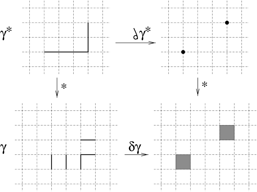
Figure 3: The relation between disorder and order correlators in a 2-D spin system. The top diagram shows a curve which defines the 2-point correlation function on the dual lattice, while the bottom diagram is the collection of links which give the disorder correlator.

As an example, consider the case of the Ising model in two dimensions. A correlation function is labeled by a set of links which start at site $i$ and end at site $j$ (see the top left diagram in Figure 3). A disorder operator on the dual lattice is obtained by interpreting the set of links joining site $i$ to site $j$ on the dual lattice. This corresponds to the links displayed in the bottom left diagram in Figure 3. Inserting the characters along each link in that diagram into the partition function computes the correlator of the two disorder operators shown in the diagram on the bottom right. Notice that they are dual to the two site variables in the top right.

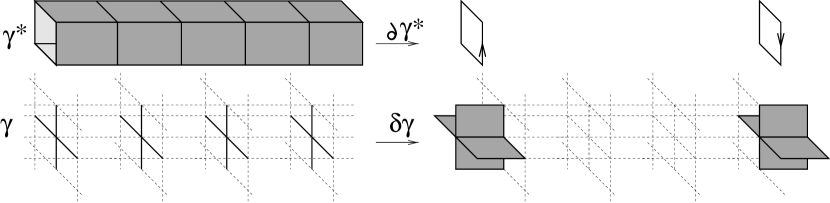
Figure 4: The relation between disorder correlators in a 3-D spin system and Wilson loops in a 3-D gauge theory. The top diagram is the surface which defines the two Wilson loops at its ends, and the lower diagram is its dual - a collection of links whose coboundary produces the disorder variables in the spin model.

As a second example consider a spin model in three dimensions. The correlator is as usual given by a set of links joining site $i$ and site $j$. A disorder correlator on the other hand is obtained by consider a set of plaquettes forming a surface on the dual lattice. We will take the example of a cylindrical like surface (see the top left diagram in Figure 4). Interpreting the surface back on the original lattice leads to a set of links forming cross like shapes (see the bottom left diagram in Figure 4). Inserting the set of characters for these links into the partition function computes the correlator of the set of disorder variables shown in the bottom right diagram of Figure 4. Once again they are dual to the correlator on the dual lattice, which in this case is the correlator of two Wilson loops.

In the remainder of this section we will demonstrate how the duality relations found in section 2.3 relates order and disorder operators. We will show that there is a class of correlators which vanish identically on topological grounds alone. Duality is in fact even more powerful, and in certain dimensions it allows one to obtain the correlation function of an arbitrary set of operators explicitly. Several explicit examples will be explored at the end of the section.

5.1 General Formalism

In the previous section the correlators were defined by inserting characters, in a particular fixed representation, on a collection of $k$-cells, $\gamma$. It is however unnecessary to fix the representations on all of the cells of $\gamma$, one can allow the representations to vary over the $k$-cells of $\gamma$. In fact, it is possible to compute such correlators explicitly in $d=k$ dimensions. That computation will be carried out shortly after the general case has been worked out.

Here, we will consider a general correlator defined by an arbitrary collection of $k$-cells denoted by $\gamma$ and a set of representations $\{S_{p}\in{\cal G}^{*}\}$ for all $p\in\gamma$. These correlators include, but are not limited to the order and disorder correlators mentioned earlier. The correlator is defined much like (5.1),

$$W(\{S_{p}\}) \equiv \left\langle\prod_{p\in\gamma}\chi_{S_{p}}\left(\langle\delta\sigma,c_{k}^{(p)}\rangle\right)\right\rangle$$ (5.3)

$$= \frac{1}{Z}\sum_{\{n_{a}\in{\cal H}_{a}\}}\sum_{\sigma\in C_{k-1}(\Omega,{\cal G})}\prod_{p\in\gamma}\chi_{S_{p}}\left(\langle\delta\sigma,c_{k}^{(p)}\rangle\right)\prod_{p=1}^{{\cal N}_{k}}B_{p}\left(\left\langle\delta\sigma+n_{a}h^{a},c_{k}^{(p)}\right\rangle\right)$$

where $Z$ is of course the partition function (2.8). The dual transformations on this correlator can be carried out in a rather trivial manner. Firstly, let $\gamma_{s}$ denote the set of $k$-cells with representation $s$, so that $\cup_{s}\gamma_{s}=\gamma$. If $\gamma_{s}$ has no boundary the correlation function of $\gamma_{s}$ reduces to the partition function. This can be seen from (5.2). Consequently, we restrict the discussion to the case where $\gamma_{s}$ has a boundary for every $s$. In that case, the product over characters can be trivially absorbed in a redefinition of the Boltzmann weight,

$$B_{p}\left(\langle\delta\sigma+n_{a}h^{a},c_{k}^{(p)}\rangle\right) \to B_{p}\left(\langle\delta\sigma+n_{a}h^{a},c_{k}^{(p)}\rangle\right)\chi_{S_{p}}\left(\langle\delta\sigma,c_{k}^{(p)}\rangle\right)$$ (5.4)

$$= \frac{1}{|{\cal G}|}\sum_{r_{p}\in{\cal G}^{*}}b_{p}(\langle r,c_{k}^{(p)}\rangle)\chi_{\langle r,c_{k}^{(p)}\rangle}(\langle\delta\sigma+n_{a}h^{a},c_{k}^{(p)}\rangle)\chi_{\langle S,c_{k}^{(p)}\rangle}(\langle\delta\sigma,c_{k}^{(p)}\rangle)$$

$$= \frac{1}{|{\cal G}|}\sum_{r_{p}\in{\cal G}^{*}}b_{p}(\langle r-S,c_{k}^{(p)}\rangle)\chi_{\langle r,c_{k}^{(p)}\rangle}(\langle\delta\sigma+n_{a}h^{a},c_{k}^{(p)}\rangle)$$

for all $p\in\gamma$ and we have defined the $k$-chain $S\equiv\sum_{s}S_{s}=\sum_{p\in\gamma}S_{p}\;c_{k}^{(p)}$. The last equality in (5.4) was obtained by using the factorization properties of the characters, (2.10), and then shifting $r$. Although the two arguments of the characters in the second line appear to be different, this difference vanishes for $p\in\gamma$ because one can always arrange for the generators of the cohomology to have no overlap with the cells of $\gamma$. To be precise $\langle S,h^{a}\rangle=0$ since a non-vanishing inner product implies that $S$ contains an element of the homology group, but this contradicts the assumption that all $\gamma_{s}$ have a boundary.

With this shift in the Boltzmann weights the dual correlator is trivial to obtain, simply use (2.18) with the appropriate character coefficients.

$$W(\{S_{p}\})=\frac{1}{Z}\sum_{\{{\widetilde{n}}_{a}\in{\cal G}^{*}\perp{\cal H}_{a}^{*}\}}\;\sum_{r\in C_{d-k-1}(\Omega^{*},{\cal G}^{*})}\;\prod_{p=1}^{{\cal N}^{*}_{d-k}}b_{p}\left(\left\langle\delta r-S^{*}+{\widetilde{n}}_{a}h^{*a},c_{d-k}^{*(p)}\right\rangle\right)$$ (5.5)

The normalizing partition function, $Z$, should be evaluated in its dual form (2.18) so that the factors of the group volume that were left out to avoid clutter throughout, do not spoil the equality. Also, $S^{*}$ is the dual to $S$, obtained by interpreting the set of $k$-cells, $\gamma,$ on the original lattice as a set $d-k$ cells, $\gamma^{*}$, on the dual lattice and defining $S^{*}=\sum_{p\in\gamma^{*}}S_{p}\;c_{d-k}^{*(p)}$. It should be clear that if $\gamma$ was chosen to define an order correlator, then (5.5) is a disorder correlator in the dual variables thus establishing the connection between strong and weak coupling, and order and disorder variables.

There is a class of correlators which this formalism does not include. These correlators correspond to inserting characters along a set of $(k-1)$-cells which form a closed sheet wrapping around a non-trivial $(k-1)$-cycle of the lattice. For example, a gauge theory on $S^{1}\times{\cal M}$, where ${\cal M}$ is a contractable space, has a Wilson loop which wraps once around the compact direction. This set of links is not the boundary of a two-dimensional sheet and hence cannot be written in the form (5.3). However, in the next section we will demonstrate that such correlators vanish identically.

5.2 The Vanishing Correlator

We now prove a powerful theorem, concerning the vanishing of certain correlators in a statistical model. The physical interpretation of the theorem will be explained, and some interesting applications will be given shortly.

Theorem: Let $\gamma$ be a collection of $(k-1)$-cells with zero boundary and $\{S_{l}\in{\cal G}^{*}\}$ a collection of representations labeled by $l\in\gamma$. If $S\equiv\sum_{l\in\gamma}S_{l}\,c_{k-1}^{(l)}$ is a representative element of $H_{k-1}(\Omega,{\cal G}^{*})$ then the following correlator vanishes identically,

$$W(\gamma)\equiv\left\langle\prod_{l\in\gamma}\chi_{S_{l}}\left(\sigma_{l}\right)\right\rangle=\frac{1}{Z}\sum_{\{n_{a}\in{\cal H}_{a}\}}\sum_{\sigma\in C_{k-1}(\Omega,{\cal G})}\;\prod_{l\in\gamma}\chi_{S_{l}}\left(\langle\sigma,c_{k-1}^{(l)}\rangle\right)\;\prod_{p=1}^{{\cal N}_{k}}\;B_{p}\left(\langle\delta\sigma+n_{a}h^{a},c_{k}^{(p)}\rangle\right)$$

where $Z$ is given by Eq.(2.8).
Proof: Introduce the character expansion of the Boltzmann weights, so that every $k$-cell carries an irreducible representation, ${\cal G}^{*}$, of the group ${\cal G}$. Encode this information into a $k$-chain denoted by $r$ and re-order the sum. The result is,

$$W(\{S_{p}\}) = \sum_{r\in C_{k}(\Omega,{\cal G}^{*})}\;\prod_{p=1}^{{\cal N}_{k}}b_{p}(\langle r,c_{k}^{(p)}\rangle)$$ (5.6)

$$\sum_{\{n_{a}\in{\cal H}_{a}\}}\;\sum_{\sigma\in C_{k-1}(\Omega,{\cal G})}\;\prod_{l\in\gamma}\chi_{S_{l}}\left(\langle\sigma,c_{k-1}^{(l)}\rangle\right)\;\prod_{p=1}^{{\cal N}_{k}}\;\chi_{\langle r,c_{k}^{(p)}\rangle}\left(\langle\delta\sigma+n_{a}h^{a},c_{k}^{(p)}\rangle\right)$$

where $b(r)$ are the character coefficients of the Boltzmann weights given in (2.9). Using (2.13) and the factorization properties of the characters, (2.10), one finds that the sum over $\sigma$ and $\{n_{a}\}$ reduces,

$$\sum_{n_{a},\sigma}\dots = \sum_{\sigma\in C_{k-1}(\Omega,{\cal G})}\;\prod_{l\in\gamma}\;\chi_{S_{l}}\left(\langle\sigma,c_{k-1}^{(l)}\rangle\right)\;\prod_{l=1}^{{\cal N}_{k-1}}\;\chi_{\langle\partial r,c_{k-1}^{(l)}\rangle}\left(\langle\sigma,c_{k-1}^{(l)}\rangle\right)\sum_{\{n_{a}\in{\cal H}_{a}\}}\prod_{a=1}^{A^{k}}\chi_{\langle\partial r,h^{a}\rangle}\left(n_{a}\right)$$ (5.7)

$$= \sum_{\sigma\in C_{k-1}(\Omega,{\cal G})}\;\prod_{l=1}^{{\cal N}_{k-1}}\;\chi_{\langle\partial r+S,c_{k-1}^{(l)}\rangle}\left(\langle\sigma,c_{k-1}^{(l)}\rangle\right)\prod_{a=1}^{A^{k}}\sum_{n_{a}\in{\cal H}_{a}}\chi_{\langle\partial r,h^{a}\rangle}\left(n_{a}\right)$$

$$= \prod_{l=1}^{{\cal N}_{k-1}}\;\delta_{{\cal G}^{*}}\left(\langle\partial r+S,c_{k-1}^{(l)}\rangle\right)\prod_{a=1}^{A^{k}}\delta_{{\cal H}_{a}^{*}}\left(\langle\partial r,h^{a}\rangle\right)$$

where we have used the orthogonality of the characters, (2.11), to obtain the last equality. If $S$ is a representative element of $H_{k-1}(\Omega,{\cal G}^{*})$ then the first delta function is forced to vanish, since by definition there exists no $k$-chain $r$ whose boundary equals an element of the homology group. Thus, the correlator (5.2) vanishes $\Box$.

Figure 5: This diagram depicts the set of plaquettes which are used in the computation of the correlator between the two Wilson loops on its boundary.

This rather general theorem has some interesting physical consequences. Consider for example a spin model ($k=1$) in arbitrary dimensions and compute the correlator of an odd number of characters. This vanishes identically from symmetry reasons alone, however, from the point of view of the above theorem it vanishes since an odd number of points is homologous to a single point, and hence is a representative element of $H_{0}(\Omega,{\cal G}^{*})$ and thus must vanish on topological grounds. A more interesting application of the theorem is to consider a gauge theory ($k=2$) on a manifold which has one compact direction, and compute the Wilson loop around that compact direction in representation $s$. This loop is clearly a representative of $H_{1}(\Omega,{\cal G}^{*})$ and thus the Wilson loop correlator must vanish identically. Although this result can be reasoned from symmetry arguments, it seems somewhat more illuminating to see how it follows from purely topological requirements. It is interesting to note that if one were to compute the correlator of two Wilson loops wrapped once around the compact direction with conjugate representations (i.e. one with representation $s$ and the other with representation $-s$) it does not vanish. The reason is because the $k$-chain $S=s(\sum_{l\in\gamma_{1}}-\sum_{l\in\gamma_{2}})$ is the boundary of a sheet formed between the two loops, $S=s\;\partial\sum_{p\in\Gamma}c_{2}^{(p)}$ where $\Gamma$ is set of plaquettes connecting one loop to the other (see Figure 5), and is hence not a representative of $H_{1}(\Omega,{\cal G}^{*})$. In fact, since the correlator is reduced to a correlator for plaquette valued objects one can use the results of section 5.1 to complete the duality transformation. We mention this since if the distance between the two loops is taken to zero such a correlator corresponds to the computation of a single Wilson loop correlator in the adjoint representation which in a non-Abelian theory does not vanish. In general there are only two fundamentally different types of correlators, those that can be written in terms of the boundary of a higher dimensional surface, which we have shown how to compute in the previous section, and those that form representative elements of the homology group, which has been demonstrated to vanish.

5.3 Correlators in $d=k$ dimensions

Since we have established that a non-vanishing correlator is of the general form (5.3), and its dual formulation (5.5), in this section we deal only with those cases. It is possible to obtain an explicit form for these correlators in $d=k$ dimensions solely in terms of the topological properties of the lattice. The reason is as follows: in performing the duality transformations the constraints (2.14) must be solved, however, in dimensions $d=k$ the most general solution to the first set of constraints in (2.14) is $r=h\in H_{d}(\Omega,{\cal G}^{*})$ because there are no $(d+1)$-chains on a $d$-dimensional lattice. Consequently, the dual theory contains only topological fluctuations. This sort of trivialization of the problem can also be seen from the point of the view of the field-strength formulation (3.4). In dimensions $d=k$ the local Bianchi constraints are absent rendering the dynamical fields locally free while constraining them only globally. Of course the form of the dual correlator (5.5) implies this trivialization as well, since when $d=k$ the dynamical field $\sigma$ is a $(-1)$-chain, which of course has only the identity element, the only sums that remain are those over $\{{\widetilde{n}}_{a}\}$. It is trivial to write down the correlators in these dimensions, and they consists of only a finite number of sums (or integrals if the dual group is continuous),

$$W(\{S_{p}\})=\frac{\sum_{\{{\widetilde{n}}_{a}\in{\cal G}^{*}\perp{\cal H}_{a}^{*}\}}\prod_{p=1}^{{\cal N}^{*}_{0}}b_{p}\left(\left\langle{\widetilde{n}}_{a}h^{*a}-S^{*},c_{0}^{*(p)}\right\rangle\right)}{\sum_{\{{\widetilde{n}}_{a}\in{\cal G}^{*}\perp{\cal H}_{a}^{*}\}}\prod_{p=1}^{{\cal N}^{*}_{0}}b_{p}\left(\left\langle{\widetilde{n}}_{a}h^{*a},c_{0}^{*(p)}\right\rangle\right)}$$ (5.8)

here $\{h^{*a}\}$ are the set of generators of $H^{0}(\Omega^{*},{\cal G}^{*})$ which are dual to the generators of the homology group $H_{d}(\Omega,{\cal G}^{*})$. In the next two sections we will use this formula to compute some non-trivial correlators in a spin model on an arbitrary graph and a gauge theory on an arbitrary orientable two-dimensional Riemann surface. These results have straightforward generalizations to the higher dimensional cases.

5.4 Spin System Case

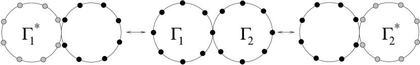
Figure 6: A one dimensional graph and its dual. The middle diagram depicts the original lattice, and $\Gamma_{i}$ are the set of links contained in the corresponding loop. The end diagrams depict the dual lattice, and the shaded sites are the duals to $\Gamma_{i}$, $\Gamma_{i}^{*}$,which generate $H^{0}(\Omega^{*},{\cal G}^{*})$.

In this section the computation of correlators in a spin model on a $1$-dimensional graph using (5.8) will be carried out. Let $\Omega$ be a one dimensional graph, and let $\{h^{*a}\}$ denote the generators of $H^{0}(\Omega^{*},{\cal G}^{*})$. To attach a physical meaning to these generators consider the generators of $H_{1}(\Omega,{\cal G}^{*})$ and then re-interpret them on the dual lattice. It should be obvious that $H_{1}(\Omega,{\cal G}^{*})$ is generated by the set of links which form closed loops on the graph (take only an independent set of these generators). Figure 6 is an illustrative example of how this works. In general the generators of $H^{0}(\Omega^{*},{\cal G}^{*})$ are $h^{a}=\sum_{i\in\Gamma^{*}_{a}}C_{0}^{(i)}$ where $\Gamma^{*}_{a}$ ($a=1,\dots,A$) is a collection points, on the dual lattice, which are dual to a set of links that form a closed loop on the original lattice. It is easy to convince oneself that the coboundary of $h^{a}$ vanishes, and since there are no lower dimensional chains this is an element of the cohomology. As long as the set of loops are independent then these generators form a complete set.

The correlation function is defined via a set of links on the original lattice, $\gamma$, and representations, $\{S_{l}\}$, for every link. When $\gamma$ is interpreted on the dual lattice it corresponds to a set of points, $\gamma^{*}$. Let $\gamma^{*}_{a}$ denote the set of points in $\gamma^{*}$ that are contained in $\Gamma^{*}_{a}$ (i.e. the set of points dual to the set of links contained in the $a$-th loop of the original lattice). Also, let $\{S_{i}^{*}\}$ denote the collection of representations on the dual sites, and define the $0$-chain ${\cal S}_{a}^{*}\equiv\sum_{i\in\gamma^{*}_{a}}S^{*}_{i}\;c_{0}^{*(i)}$. Applying the dual formulation of the correlator (Eq.(5.8)), represented by $\gamma$ gives,

$$W(\{S_{p}\})=\prod_{a=1}^{A}\left\{\frac{\sum_{{\widetilde{n}}_{a}\in{\cal G}^{*}\perp{\cal H}_{a}^{*}}\prod_{i\in\Gamma_{a}^{*}}b_{i}\left(n_{a}-\left\langle{\cal S}_{a}^{*},c_{0}^{*(i)}\right\rangle\right)}{\sum_{{\widetilde{n}}_{a}\in{\cal G}^{*}\perp{\cal H}_{a}^{*}}\prod_{i\in\Gamma_{a}^{*}}b_{i}\left({\widetilde{n}}_{a}\right)}\right\}$$ (5.9)

We have made the assumption that the generators have no overlap, i.e. $\Gamma_{a}\cap\Gamma_{b}=\emptyset$ if $a\neq b$. It is not difficult to include the cases where there are overlaps, however, this only serves to complicate the final sums over $\{n_{a}\}$. It is possible to simplify the summations in the above expression only once the Boltzmann weights are specified. A convenient example is furnished by choosing ${\cal G}=U(1)$ and the Villan form for the Boltzmann weight, so that,

$$b_{i}({\widetilde{n}})=\frac{1}{\sqrt{2\pi\beta}}\exp\left\{-\frac{1}{2\beta}{\widetilde{n}}^{2}\right\}$$ (5.10)

The sums over ${\widetilde{n}}_{a}$ can now be performed in terms of well known special functions, the Jacobi Theta function [18]. To perform the sum it is also necessary to specify $\{{\cal H}_{a}\}$. Since ${\cal G}$ was taken to be $U(1)$ this forces ${\cal H}_{a}$ to be a cyclic group, $Z\!\!\!Z_{N_{a}}$. Inserting the above ansatz into Eq.(5.9) one finds,

$$W(\{S_{p}\})$$ (5.11)

$$=\prod_{a=1}^{A}\left[\exp\left\{-\frac{1}{2\beta}\sum_{i\in\gamma^{*}_{a}}S_{i}^{2}\right\}\frac{\sum_{{\widetilde{n}}\in Z\!\!\!Z}\exp\left\{-(2\beta)^{-1}N^{*}_{0,a}N^{2}_{a}{\widetilde{n}}^{2}+\beta^{-1}N_{a}{\widetilde{n}}\sum_{i\in\gamma_{a}^{*}}S_{i}\right\}}{\sum_{{\widetilde{n}}\in Z\!\!\!Z}\exp\left\{-(2\beta)^{-1}N^{*}_{0,a}N^{2}_{a}{\widetilde{n}}^{2}\right\}}\right]$$

$$=\prod_{a=1}^{A}\left[\exp\left\{-\frac{1}{2\beta}\left(\sum_{i\in\gamma_{a}^{*}}S_{i}^{2}-\frac{1}{{\cal N}_{0,a}^{*}}\left(\sum_{i\in\gamma_{a}^{*}}S_{i}\right)^{2}\right)\right\}\frac{\theta_{3}\left(\frac{2\beta}{N_{a}^{2}{\cal N}_{0,a}^{*}};-\frac{1}{N_{a}{\cal N}_{0,a}^{*}}\sum_{i\in\gamma_{a}^{*}}S_{i}^{*}\right)}{\theta_{3}\left(\frac{2\beta}{N^{2}{\cal N}_{0,a}^{*}};0\right)}\right]$$

Here ${\cal N}_{0,a}^{*}$ denotes the number of sites on the dual lattice contained in $\Gamma_{a}^{*}$. This general formula is not extremely illuminating, however, it reduces to a reasonable form for the two point function. In that case $\gamma$ consists of a set of links which form a single continuous path from point $i$ to $j$ on the lattice and the representations on those links are all taken to be labeled by $s$. Then the above expression reads,

$$W(\{s\})=\prod_{a=1}^{A}\left[\exp\left\{-\frac{s^{2}}{2\beta}\;\frac{L(\gamma^{*}_{a})({\cal N}_{0,a}^{*}-L(\gamma^{*}_{a}))}{{\cal N}_{0,a}^{*}}\right\}\frac{\theta_{3}\left(\frac{2\beta}{N_{a}^{2}{\cal N}_{0,a}^{*}};-\frac{s\;L(\gamma_{a}^{*})}{N_{a}{\cal N}_{0,a}^{*}}\right)}{\theta_{3}\left(\frac{2\beta}{N_{a}^{2}{\cal N}_{0,a}^{*}};0\right)}\right]$$ (5.12)

where $L(\gamma_{a}^{*})$ is the number of dual sites (links) contained in $\gamma_{a}^{*}$ ($\gamma_{a}$) and counts the number of links that the path $\gamma$ crossed in going through the $a$-th loop of the graph. Notice that the overall exponential factor is explicitly invariant under,

$$L(\gamma_{a}^{*})\to{\cal N}_{0,a}^{*}-L(\gamma_{a}^{*})$$ (5.13)

This symmetry implies that the overall factor is not affected by which path one took in going through a loop. However, the theta-function contributions are invariant only under an integer shift in the second parameter. Write $s=s_{1}+Ns_{2}$ where $s_{1}\in\{0,\dots,N-1\}$, $s_{2}\in Z\!\!\!Z$ and $N$ is the lowest common factor of $\{N_{a}\}$. It is clear that under the transformation (5.13), the theta function is invariant only if $s_{1}=0$. In general for a fixed $s_{2}$ there are $N$ inequivalent sectors of the model, each sector transforms differently under the transformation (5.13). The appearance of these sectors can be traced back to the discussion in section 3.2. It was pointed out there that performing the sum over topological sectors, $\{n_{a}\}$, in a subgroup of the gauge group introduces fractional global charge into the system. In computing the two-point function one is forced to introduce a set of links forming a path with two end points. Naively, the choice of path has no effect on the correlator, however, due to the existence of fractional charge in the system there are lines of flux which pierce through the path. Consequently, a different choice of path carries a different amount of fractional charge, leading to a non-trivial transformation of the correlator under the transformation (5.13). Only when the representation of the path respects the $n$-ality of the global charges can the system be symmetric under (5.13). This requirement forces the representation $s$ to be an integer multiple of the lowest common multiple of the global charges which it is exposed to.

5.5 Gauge Theory Case

We now consider an Abelian gauge theory ($k=2$), with gauge group ${\cal G}$, on an arbitrary orientable two-dimensional Riemann surface. Let $\Omega$ be a discretetization of this manifold. Since the generator of the second homology group is the entire surface, this implies that $H^{0}(\Omega,{\cal G}^{*})$ has one generator which is given by $h=\sum_{i\in\Omega^{*}}c_{0}^{*(i)}$. The correlator (5.3) then reduces to,

$$W(\{S_{p}\})=\frac{\sum_{{\widetilde{n}}\in{\cal G}^{*}\perp{\cal H}^{*}}\prod_{i=1}^{{\cal N}^{*}_{0}}b_{i}\left({\widetilde{n}}-\left\langle S^{*},c_{0}^{*(i)}\right\rangle\right)}{\sum_{{\widetilde{n}}\in{\cal G}^{*}\perp{\cal H}^{*}}\prod_{i=1}^{{\cal N}^{*}_{0}}b_{i}\left({\widetilde{n}}\right)}$$ (5.14)

As in the last section consider ${\cal G}=U(1)$, ${\cal H}=Z\!\!\!Z_{N}$ and the Boltzmann weight in Villan form (5.10). Then Eq.(5.14) reduces to,

$$W(\{S_{p}\})=\exp\left\{-\frac{1}{2\beta}\left(\sum_{i\in\gamma^{*}}(S_{i}^{*})^{2}-\frac{1}{{\cal N}_{0}^{*}}\left(\sum_{i\in\gamma^{*}}S_{i}^{*}\right)^{2}\right)\right\}\frac{\theta_{3}\left(\frac{2\beta}{N^{2}{\cal N}_{0}^{*}};-\frac{1}{N{\cal N}_{0}^{*}}\sum_{i\in\gamma^{*}}S_{i}^{*}\right)}{\theta_{3}\left(\frac{2\beta}{N^{2}{\cal N}_{0}^{*}};0\right)}$$ (5.15)

The simplest correlator in a gauge theory is a (filled) Wilson loop, in which $\gamma$ is a collection of adjacent plaquettes and $\{S_{p}=s\}$ (the two loops in Figure 5 is one such example). Equation (5.15) then becomes,

$$W(\{s\})=\exp\left\{-\frac{s^{2}}{2\beta}\;\frac{A(\gamma^{*})({\cal N}_{0}^{*}-A(\gamma^{*}))}{{\cal N}_{0}^{*}}\right\}\frac{\theta_{3}\left(\frac{2\beta}{N^{2}{\cal N}_{0}^{*}};-\frac{s~{}A(\gamma^{*})}{N{\cal N}_{0}^{*}}\right)}{\theta_{3}\left(\frac{2\beta}{N^{2}{\cal N}_{0}^{*}};0\right)}$$ (5.16)

Here $A(\gamma^{*})$ denotes the number of dual sites (plaquettes) contained in $\gamma^{*}$ ($\gamma$). Just as in the spin model case the exponential is invariant under the following transformation,

$$A(\gamma^{*})\to{\cal N}_{0}^{*}-A(\gamma^{*})$$ (5.17)

This symmetry implies that the exponential part of the correlation function does not distinguish between what is consider the inside or outside area of the Wilson loop. Notice that in the limit in which the area of the surface becomes infinite while the area of the Wilson loop remains finite ($A(\gamma^{*})/{\cal N}_{0}^{*}\to 0$) the exponential reduces to the familiar area law. However, if the ratio of the number of plaquettes in the Wilson loop and the total number of plaquettes on the manifold is kept fixed ($A(\gamma^{*})/{\cal N}_{0}^{*}={\rm const.}$) as the number of plaquettes is taken to infinity, so that one reproduces the continuum limit, then there are finite size corrections given both by the theta-function and the overall exponential.

As in the spin model scenario, the theta-function does not respect the symmetry (5.17) in general. The generic case has $s=s_{1}+Ns_{2}$ where $s_{1}\in\{0,\dots,N-1\}$ and $s_{2}\in Z\!\!\!Z$, if $s_{1}\neq 0$ the system distinguishes between inside and out of the loop, just as in the one-dimensional spin model. The reasoning follows through much like it did there. The fractional charge induces a flux which is incompatible with the representation (unless $s=NZ\!\!\!Z$) and as such a different choice of surface carries a different amount of flux. The $N$ different sectors are once again seen to give rise to $N$ different transformations of the correlator under (5.17). This bears a strong resemblance to the appearance of theta sectors in non-Abelian gauge theories. It indicates that there is a strong connection between theta sectors in a non-Abelian theory, and the topological sectors in an appropriate Abelian model on a topologically non-trivial manifold.

Before closing we would like to illustrate how one can include direct product groups in a rather trivial manner. As an example consider the case in which the gauge group ${\cal G}=\oplus_{a=1}^{m}U(1)$ and ${\cal H}=\oplus_{a=1}^{m}Z\!\!\!Z_{N_{m}}$. Also choose the heat kernel action,

$$b_{i}(({\widetilde{n}}^{1},\dots,{\widetilde{n}}^{m}))=\prod_{a=1}^{m}\frac{1}{\sqrt{2\pi\beta_{a}}}\exp\left\{-\frac{1}{2\beta_{a}}(n^{a})^{2}\right\}$$

here $\{\beta_{a}\}$ are independent coupling constants. Since the gauge group is a product group it is necessary to specify multiple representations of $U(1)$ on every plaquette in $\gamma$, label these representations by $\{S_{p}^{a}\}$. Since the Boltzmann weights have no cross terms the problem factorizes and the correlation function is straightforward to write down,

$$W(\{S^{a}_{p}\})=\prod_{a=1}^{m}\left[\exp\left\{-\frac{1}{2\beta_{a}}\left(\sum_{i\in\gamma^{*}}(S^{*a}_{i})^{2}-\frac{1}{{\cal N}_{0}^{*}}\left(\sum_{i\in\gamma^{*}}S^{*a}_{i}\right)^{2}\right)\right\}\frac{\theta_{3}\left(\frac{2\beta_{a}}{N^{2}_{a}{\cal N}_{0}^{*}};-\frac{1}{N_{a}{\cal N}_{0}^{*}}\sum_{i\in\gamma}S^{*a}_{i}\right)}{\theta_{3}\left(\frac{2\beta_{a}}{N^{2}_{a}{\cal N}_{0}^{*}};0\right)}\right]$$

Once again consider the simplifying case of a filled Wilson loop in which $\{S_{p}^{a}=s\}$ for all $p\in\gamma$. The above expression then reduces to a product of factors like that appearing in (5.16),

$$W(\{s\})=\exp\left\{-\frac{s^{2}}{2{\tilde{\beta}}{\cal N}_{0}^{*}}\;A(\gamma)({\cal N}_{0}^{*}-A(\gamma))\right\}\prod_{a=1}^{m}\left(\frac{\theta_{3}\left(\frac{2\beta_{a}}{N^{2}_{a}{\cal N}_{0}^{*}};-\frac{s~{}A(\gamma)}{N_{a}{\cal N}_{0}^{*}}\right)}{\theta_{3}\left(\frac{2\beta_{a}}{N^{2}_{a}{\cal N}_{0}^{*}};0\right)}\right)$$ (5.18)

where ${\tilde{\beta}}=\sum_{a=1}^{m}\beta_{a}^{-1}$. The invariance of this expression under $A(\gamma)\to{\cal N}_{0}^{*}-A(\gamma)$ depends upon whether $s$ is a representation which respects the $n$-ality of the fractional charge. In this case only if $s\in NZ\!\!\!Z$ where $N$ is the least common multiple of $\{N_{a}\}$ will the expression be invariant under that symmetry.

6 Conclusions

We have introduced some new statistical models in which a sum over various topological sectors of the system were included. The dual model was constructed explicitly, and several useful examples were presented, making connection with the usual notations and conventions. Using this duality transformation the model was written in terms of the natural field-strength variables which were found to be constrained by local and global Bianchi identities. This formulation of model was derived in a gauge-invariant manner and the sum over the topological sectors were seen to introduce fractional charges along the non-trivial $k$-cycles of the lattice. The fact that it is possible to introduce a sum over different groups for the different $k$-cycles was used to form self-dual models in which there were several distinct global charges in the system. These are new self-dual models and the analysis of [19] could be used to identify the self-dual points in these models as possible new critical points. Finally, the duality transformations were carried out on correlation functions in various dimensions. We proved that a certain subset of correlators vanished identically, in addition it was shown how correlators in dimensions $d=k$ are completely determined by the duality transformation in terms of the topological modes of the theory.

7 Acknowledgments

The author would like to thank T. Fugleberg, L. D. Paniak, O. Tirkkonen, G. W. Semenoff and A. Zhitnitsky for useful discussions on various aspects of this paper. The hospitality of the Niels Bohr Institute, where part of this work was completed, was also much appreciated.

References

- [1]
- [2] N. Seiberg and E. Witten, Nucl. Phys. B426 (1994) 19.
- [3] N. Seiberg and E. Witten, Nucl. Phys. B431 (1994) 484.
- [4] H. A. Kramers and G. H. Wannier, Phys. Rev. 60 (1941) 252.
- [5] R. Savit, Rev. Mod. Phys. 52 (1980) 453.
- [6] E. Fradkin and L. Susskind, Phys. Rev. D17 (1978) 2637.
- [7] C. R. Gattringer, S. Jaimungal, G. W. Semenoff, Phys. Lett. B425 (1998) 282.
-
[8]
M. Rakowski, Phys. Rev. D52 (1995)
354;
M. Rakowski and S. Sen, Lett. Math. Phys. 42 (1997) 195. - [9] K. Drühl and H. Wagner, Ann. Phys. 141 (1982) 225.
- [10] I. Halperin and A. Zhitnitsky, hep-ph/9711398.
- [11] M. A. Shifman and A. I. Vainshtein, Nucl. Phys. B296 (1988) 445.
- [12] A. Kovner and M. A. Shifman, Phys. Rev. D56 (1997) 2396.
- [13] M. B. Halpern, Phys. Rev. D19 (1979) 517.
-
[14]
G. G. Batrouni,
Nucl. Phys. B208 (1982) 467;
G. G. Batrouni, Nucl. Phys. B208 (1982) 12;
G. G. Batrouni and M. B. Halpern, Phys. Rev. D30 (1984) 1775;
G. G. Batrouni and M. B. Halpern, Phys. Rev. D30 (1984) 1782. - [15] E. H. Spanier, Algebraic Topology, Springer-Verlag, 1966.
- [16] S. Jaimungal, hep-th/9805211. To appear in Phys. Lett. B.
- [17] B. Rusakov, Nucl. Phys. B507 (1997) 691.
- [18] J. Spanier and K. B. Oldham, An Atlas of Functions, Hemisphere Publishing Corporation, New York (1987).
- [19] P. H. Damgaard and P. E. Haagensen, J. Phys. A30 (1997) 4681.