Quantum Inhomogeneities in String Cosmology

Abstract

Within two specific string cosmology scenarios –differing in the way the pre- and post-big bang phases are joined– we compute the size and spectral slope of various types of cosmologically amplified quantum fluctuations that arise in generic compactifications of heterotic string theory. By further imposing that these perturbations become the dominant source of energy at the onset of the radiation era, we obtain physical bounds on the background’s moduli, and discuss the conditions under which both a (quasi-) scale-invariant spectrum of axionic perturbations and sufficiently large seeds for the galactic magnetic fields are generated. We also point out a potential problem with achieving the exit to the radiation era when the string coupling is near its present value.

I Introduction

Perhaps the most appealing feature of standard inflationary cosmology [1] is its ability to stretch out generic/arbitrary initial classical inhomogeneities and to replace them by a calculable spectrum of cosmologically amplified quantum fluctuations. The latter behave, for all physical purposes, as a set of properly normalized stochastic classical perturbations. A much advertised outcome of slow-roll inflation is a (quasi-) scale-invariant (Harrison-Zeldovich (HZ)) spectrum of density fluctuations, a highly desirable feature for explaining both the CMB temperature fluctuations on large angular scales and the large-scale structure of the visible part of our Universe.

The so-called pre-big bang (PBB) scenario [2, 3] offers, within the context of string theory, an alternative to the usual inflationary paradigm. Provided a graceful exit can be achieved  (see [4, 5] for recent progress on this issue), the PBB scenario exhibits several appealing advantages, e.g.

• it naturally provides inflationary solutions through the duality symmetries [6] of string theory;

• it assumes a natural, simple, initial state for the Universe, which is fully under control: the perturbative vacuum of superstring theory;

• it needs no fine-tuning of couplings and/or potentials: the inflaton is identified with the dilaton, which is ubiquitous in string theory, is effectively massless at weak coupling, and provides inflation through its kinetic energy;

• it can provide a hot big bang initial state as a late-time outcome of the pre-big bang phase, through the amplification of vacuum quantum fluctuations generated in this latter phase.

In recent work [7, 8] we have discussed the conditions under which classical inhomogeneities get efficiently erased in string cosmology. In general, this does occur provided two moduli of the classical solutions at weak coupling and curvature (basically an initial coupling and an initial curvature scale) are bounded from above. Whether such conditions correspond to an acceptable degree of fine-tuning of the initial conditions or not is still the matter of some controversy [9, 10, 8].

An interesting outcome of these investigations has been a motivated conjecture [8] that, for negative spatial curvature, the pre-big bang phase itself is generically preceded by a contracting “Milne” phase, corresponding to a particular parametrization of the past light cone of trivial Minkowski space-time with a constant dilaton. Such a background, the trivial all-order classical vacuum of superstring theory, turns out to be an unstable early-time fixed point of the evolution. Thanks to dilaton/metric fluctuations, it appears to lead, inevitably, to pre-big bang-type inflation at later times.

In this paper we shall assume that the above classical picture effectively wipes out, during its long pre-big bang phase, spatial curvature and classical inhomogeneities, and we move on to analyse the second alleged virtue of inflationary cosmology, the generation of an interesting spectrum of amplified quantum fluctuations. As several previous investigations have shown [11, 12, 13], achieving this is not at all automatic in string cosmology. It was soon realized that, in the simplest PBB scenario, tensor  [11] and scalar-dilaton [12] perturbations tend to have steep spectra (typically a spectral index $n=4$, as compared to HZ’s $n=1$). Perturbations of gauge fields coming from compactification of the extra 16 bosonic dimensions of heterotic string theory can have somewhat smaller spectral indices [13], but still in the range $3<n<4$.

The situation can be improved by assuming [11] that a long string phase (during which the dilaton grew linearly in cosmic time while the Universe expanded exponentially) took place between the dilaton and the usual FRW phase. In such a case, it is possible to get either an interesting spectrum of gravitational waves [11] in the range of interest for detection, or enough EM perturbations to explain the magnetic fields [13], but not both, apparently. A flat spectrum of EM perturbations, which can possibly provide a new mechanism for generating large scale structure [14] is not excluded either.

Recently, however, Copeland et al. [15] made the interesting observation that axionic perturbations, even in the absence of a string phase, can have a flat spectrum, depending on how the internal dimensions evolve during the dilatonic phase. Unfortunately, Copeland et al. stopped short of computing the axionic spectrum after re-entry. Nonetheless, their result hints at a possible dominance of axionic perturbations over all others and calls for a revision of the whole scenario and of the phenomenological constraints that must be imposed on it.

In this paper we analyse quantum fluctuations of various kinds in two distinct scenarios for the background, with or without an intermediate string phase. We may expect either possibility to occur, depending on the precise mechanism providing the transition (exit) from the PBB phase into the FRW phase.

An intermediate string phase is natural if we assume [4] that $\alpha^{\prime}$ corrections provide a non-perturbative fixed point with a high constant curvature and a linearly growing dilaton. In this case we expect the transition to the FRW phase to occur during the string phase as soon as the energy stored in the quantum fluctuations reaches criticality (recall that the condition of criticality depends on the coupling). This is like saying that the final transition to the radiation-dominated era will be induced by string-loop, back-reaction effects (see, e.g. [5]).

We can imagine, instead, that $\alpha^{\prime}$ corrections are sufficient to provide by themselves a sudden branch-change from the perturbative PBB phase to another duality-related vacuum phase, with the Hubble parameter making a bounce around its maximal value. In the language of [4] this would correspond to a square-root-type vanishing of a $\beta$-function. Again, the dual ($-$ branch) phase will gently yield to a FRW Universe as soon as the energy stored in the quantum fluctuations becomes critical.

As already mentioned, an important ingredient of our approach is the (self-consistency) requirement of criticality at the beginning of the radiation era. This provides a new relation between the moduli of the PBB background and the coupling and energy density (or temperature) at the beginning of the radiation era. As we will see, the dilaton at the beginning of this era is generically displaced from its eventual/present value; hence this primordial radiation era is not yet quite the one of standard cosmology. It may take a while before the non-perturbative dilaton potential makes its presence felt and forces the dilaton to its minimum. The detailed study of such post-big bang phase is left to further work.

One of the main conclusions of this paper is that, provided $U(1)_{em}$ has a component in the Kaluza-Klein gauge group produced in the compactification from $D=10$ to $D=4$, sufficiently large seeds for galactic magnetic fields can be generated, even in the absence of a string phase. Furthermore, this happens in the same range of moduli for which a nearly scale-invariant spectrum of axionic perturbations is generated. Such a range includes a particularly symmetric point in moduli space, the one corresponding to isotropy (up to T-duality transformations) in all nine spatial dimensions.

The outline of the paper is as follows: In Sec. II we give, for the sake of completeness, the four-dimensional low-energy string-level heterotic effective action that we will work with. In Sec. III we fix our parametrization of the backgrounds for the two previously discussed scenarios. In Sec. IV we derive general formulae for the spectra of various perturbations, which get amplified by a generic background of the kind discussed in Sec. III. We will verify that our spectra satisfy a “duality” symmetry that can be shown to follow from general arguments [16]. In Sec. V we give the explicit form of the spectra for the two backgrounds discussed in Sec. III, and present them in various tables and plots. We will also impose the criticality condition and discuss its immediate consequences. Finally, Sec. VI contains a discussion of the results and some conclusions.

This paper is somewhat technical in nature and contains explicit general formulae that can be useful to the practitioner but do not carry easy messages: these can be better found in the tables and figures. At any rate, in order to help the reader, we have relegated the most complicated formulae to an appendix.

II String effective action from dimensional reduction

Following the notations of [17] we consider superstring theory in a space-time ${\cal M}\times{\cal K}$, where ${\cal M}$, with Minkowskian signature, has four non-compact dimensions, and ${\cal K}$ consists of six compact dimensions upon which all fields are assumed to be independent. Local coordinates of ${\cal M}$ are labelled by $\mu,\nu,\rho=0,\dots,3$, those of ${\cal K}$ by $a,b,c=4,\dots,9$. Moreover, all ten-dimensional fields and indices are distinguished by a hat.

We will limit ourselves to the case of a diagonal metric for the internal six-dimensional compact space, of a non-vanishing internal antisymmetric-tensor and of one Abelian heterotic $U(1)$ gauge field $A_{\mu}$:

$$\hat{g}_{\hat{\mu}\hat{\nu}}=\left(\begin{array}[]{cc}g_{\mu\nu}+g_{ab}\,V_{\mu}^{\,\,a}\,V_{\nu}^{\,\,b}&g_{ab}\,V_{\mu}^{\,\,b}\\ g_{ab}\,V_{\nu}^{\,\,b}&g_{ab}\\ \end{array}\right)\,,$$ (1)

$$\hat{B}_{\hat{\mu}\hat{\nu}}=\left(\begin{array}[]{cc}B_{\mu\nu}&W_{\mu a}-B_{ab}\,V_{\mu}^{\,\,b}\\ -W_{\nu a}+B_{ab}\,V_{\nu}^{\,\,b}&B_{ab}\\ \end{array}\right)\,.$$ (2)

In the following we take $g_{ab}=e^{2\sigma_{a}}\,\delta_{ab}$.

The low-energy four-dimensional effective string action is

$${\cal S}^{B}_{\rm eff}=\frac{1}{2\lambda_{s}^{2}}\,\int d^{4}x\,\sqrt{-g}\,e^{-\varphi}\,\left[{\cal R}+g^{\mu\nu}\,\partial_{\mu}\varphi\,\partial_{\nu}\varphi-\,g^{\mu\nu}\,\partial_{\mu}\sigma_{a}\,\partial_{\nu}\sigma_{a}-\frac{1}{4}\,e^{2\sigma_{a}}\,V_{\mu\nu}^{\,\,\,\,a}\,V^{\mu\nu a}\right.$$ (3)

$$\left.-\frac{1}{4}\,e^{-2\sigma_{a}}\,H_{\mu\nu a}\,H^{\mu\nu}_{\,\,\,\,\,a}-\frac{1}{12}\,H_{\mu\nu\rho}\,H^{\mu\nu\rho}+\frac{1}{4}F_{\mu\nu}\,F^{\mu\nu}-\frac{1}{4}\,g^{\mu\nu}e^{-2\sigma_{b}}\,e^{-2\sigma_{c}}\,\partial_{\mu}B_{bc}\,\partial_{\nu}B_{bc}\right]\,,$$ (4)

where $\lambda_{s}=\sqrt{8\pi}/M_{s}$ is the string-length parameter,

$$H_{\mu\nu\rho}=\partial_{\mu}B_{\nu\rho}-\frac{1}{2}\,\left[V_{\mu}^{\,\,a}\,W_{\nu\rho a}+W_{\mu a}\,V_{\nu\rho}^{\,\,\,\,a}\right]-\frac{1}{2}A_{\mu}\,F_{\nu\rho}+\quad\mbox{cyclic perm.}\,,$$ (5)

$$H_{\mu\nu a}=W_{\mu\nu a}-B_{ab}\,V_{\mu\nu}^{\,\,\,\,b}\,,\quad\quad F_{\mu\nu}=\partial_{\mu}A_{\nu}-\partial_{\nu}A_{\mu}\,,$$ (6)

$$V_{\mu\nu}^{\,\,\,\,a}=\partial_{\mu}V_{\nu}^{\,\,a}-\partial_{\nu}V_{\mu}^{\,\,a}\,,\quad\quad W_{\mu\nu a}=\partial_{\mu}W_{\nu a}-\partial_{\nu}W_{\mu a}\,,$$ (7)

and $\varphi$ stands for the effective four-dimensional dilaton field:

$$\varphi=\phi-\sum_{a}\sigma_{a}\,.$$

The components of the antisymmetric tensor $H^{\mu\nu\rho}$ with $\mu,\nu,\rho=0,1,2,3$ can be rewritten in terms of the pseudoscalar axion $A$ as

$$H^{\mu\nu\rho}\equiv E^{\mu\nu\rho\sigma}\,e^{\varphi}\,\partial_{\sigma}A\,,$$ (8)

where $E^{\mu\nu\rho\sigma}$ is the covariant full antisymmetric Levi-Civita tensor, which satisfies ${\cal D}_{\alpha}E^{\mu\nu\rho\sigma}=0$. Using Eq. (5), and imposing the Bianchi identity ($d^{2}B=0$), we get the equation of motion for the axion field

$$\partial_{\mu}(e^{\varphi}\,\sqrt{-g}\,g^{\mu\nu}\,\partial_{\nu}A)-\frac{1}{8}\,\frac{\epsilon^{\mu\nu\rho\sigma}}{\sqrt{-g}}\,\left[2W_{\mu\nu a}\,V_{\rho\lambda}^{\,\,\,\,a}+F_{\mu\nu}\,F_{\rho\sigma}\right]=0\,.$$ (9)

The reduced action then becomes

$${\cal S}^{A}_{\rm eff}=\frac{1}{2\lambda_{s}^{2}}\,\int d^{4}x\,\sqrt{-g}\,e^{-\varphi}\,\left[{\cal R}+g^{\mu\nu}\,\partial_{\mu}\varphi\,\partial_{\nu}\varphi-\,g^{\mu\nu}\,\partial_{\mu}\sigma_{a}\,\partial_{\nu}\sigma_{a}-\frac{1}{4}\,e^{2\sigma_{a}}\,V_{\mu\nu}^{\,\,\,\,a}\,V^{\mu\nu a}\right.$$ (10)

$$\left.-\frac{1}{4}\,e^{-2\sigma_{a}}\,H_{\mu\nu a}\,H^{\mu\nu}_{\,\,\,\,\,a}-\frac{1}{2}\,e^{2\varphi}\,g^{\mu\nu}\,\partial_{\mu}A\,\partial_{\nu}A-\frac{1}{8}\,e^{\varphi}\,\frac{A\,\epsilon^{\mu\nu\rho\sigma}}{\sqrt{-g}}\,\left[2W_{\mu\nu a}\,V_{\rho\lambda}^{\,\,\,\,a}+F_{\mu\nu}\,F_{\rho\sigma}\right]\right.$$ (11)

$$\left.+\frac{1}{4}F_{\mu\nu}\,F^{\mu\nu}-\frac{1}{4}\,g^{\mu\nu}e^{-2\sigma_{b}}\,e^{-2\sigma_{c}}\,\partial_{\mu}B_{bc}\,\partial_{\nu}B_{bc}\right]\,.$$ (12)

We are interested in fluctuations around a homogeneous background with $\varphi=\varphi(t)$,

$$g_{\mu\nu}=(-1,a^{2}(t)\,\delta_{ij},b_{c}^{2}(t)\,\delta_{cd})\,,\quad\quad i,j=1,2,3\,,\quad\quad c,d=4,\dots,9\,,\quad\quad\mbox{\rm all other fields}=0\,.$$

In the following we will also use the metric $g_{\mu\nu}=(-a^{2}(\eta),a^{2}(\eta)\delta_{ij},b_{c}^{2}(\eta)\,\delta_{dc})$, where we have introduced the conformal time $\eta$ by $d\eta=dt/a$.

III Two models for the background

If the initial value of the string coupling is sufficiently small, it is possible for the Universe to reach the high curvature regime, where higher-derivative corrections are important, while the string coupling is still small enough to neglect loop corrections ($g=\exp\varphi/2\ll 1$). As discussed in the introduction, we will consider two extreme alternatives. In the first, $\alpha^{\prime}$ corrections “lock” the Universe in a string phase with a constant $H$ and a linearly growing dilaton (with respect to cosmic time) [4]; in the second scenario, $\alpha^{\prime}$ corrections induce a sudden transition from a perturbative $(+)$ branch solution to a perturbative $(-)$ branch phase. We will refer to the latter as the dual-dilaton phase.

We will thus consider a PBB cosmological background in which the Universe starts in the perturbative string vacuum, reaches the string curvature scale while in a dilaton-vacuum solution, goes either to the dual-dilaton phase or to the string phase, and finally enters the radiation era as a result of the back-reaction from the amplified quantum fluctuations. We now parametrize these two scenarios for the backgrounds, imposing the continuity of $a,a^{\prime}$, $b_{a},b_{a}^{\prime}$, $\varphi$.

A Intermediate dual dilaton phase

• Dilaton phase

  For $-\infty<\eta<\eta_{s}$, with $\eta_{s}<0$ we have

  $$a(\eta) = -\frac{1}{H_{s}\,\eta_{s}}\,\left|\frac{\eta\,(1-\delta)-\eta_{s}}{\delta\,\eta_{s}}\right|^{\delta/(1-\delta)}\,,$$ (13)

  $$b_{a}(\eta) = -{H_{s}\,\eta_{s}}\,\left|\frac{(\eta-\eta_{s})\,(1-\delta)-\beta_{a}\,\eta_{s}}{\beta_{a}\,\eta_{s}}\right|^{\beta_{a}/(1-\delta)}=e^{\sigma_{a}}\,,$$ (14)

  $$\varphi(\eta) = \varphi_{s}+\frac{3\delta-1}{1-\delta}\log\left|\frac{\eta\,(1-\delta)-\eta_{s}}{\delta\,\eta_{s}}\right|\,,$$ (15)

  $$1 = 3\delta^{2}+\sum_{a}\beta_{a}^{2}\,,$$ (16)

  where $H_{s}=a^{\prime}(\eta_{s})/a^{2}(\eta_{s})$ is of order $M_{s}$. We will consider the case $\delta<0$ and $\beta_{a}>0$, i.e. a superinflationary solution with contracting internal dimensions. Because of the constraint between $\delta$ and $\beta_{a}$, if $|\delta|<1/\sqrt{3}$, some of the $\beta_{a}$ must be non-vanishing. In what follows we will pick two extreme cases: i) the most isotropic case, with $\beta_{a}=\sqrt{(1-3\delta^{2})/6}$, or ii) the most anisotropic one, with $\beta_{a}=\delta_{a1}\sqrt{(1-3\delta^{2})}$. In figures we shall denote these two cases by a subscript $6$ and $1$, respectively.

• Dual-dilaton phase

  For $\eta_{s}<\eta<\eta_{1}$, with $\eta_{1}>0$ we take

  $$a(\eta) = -\frac{1}{H_{s}\,\eta_{s}}\,\left|\frac{\eta\,(1-\theta)-\eta_{s}}{\theta\,\eta_{s}}\right|^{\theta/(1-\theta)}\,,$$ (17)

  $$b_{a}(\eta) = -{H_{s}\,\eta_{s}}\,\left|\frac{(\eta-\eta_{s})\,(1-\theta)-\xi_{a}\,\eta_{s}}{\xi_{a}\,\eta_{s}}\right|^{\xi_{a}/(1-\theta)}\,,$$ (18)

  $$\varphi(\eta) = \varphi_{s}+\frac{3\theta-1}{1-\theta}\log\left|\frac{\eta\,(1-\theta)-\eta_{s}}{\theta\,\eta_{s}}\right|\,,$$ (19)

  where $3\theta^{2}+\sum_{a}\xi_{a}^{2}=1$ and we will fix $\theta>0$ and $\xi_{a}<0$, i.e. a decelerated expansion for the external scale factor and a decelerated contraction for the internal ones. Again, we distinguish two cases, $\xi_{a}=-\sqrt{(1-3\theta^{2})/6}$ or $\xi_{a}=-\delta_{a1}\sqrt{(1-3\theta^{2})}$.

• Radiation phase

  In the region $\eta_{1}<\eta<\eta_{\rm eq}$, with $\eta_{\rm eq}$ the time of equivalence between radiation and matter density, we write

  $$a(\eta) = \frac{(\eta-\eta_{1}-\eta_{s})}{H_{s}\,\eta^{2}_{s}}\,\left|\frac{\eta_{1}\,(1-\theta)-\eta_{s}}{\theta\,\eta_{s}}\right|^{\theta/(1-\theta)}\,,$$ (20)

  $$\varphi(\eta) = \mbox{\rm const.}\,,\quad\quad b_{a}(\eta)=\mbox{\rm const.}\,$$ (21)

B Intermediate string phase

• Dilaton phase

  We parametrize this phase exactly as before. Thus, for $-\infty<\eta<\eta_{s}<0$, Eqs. (13) to (3.4) hold.

• String phase

  For $\eta_{s}<\eta<\eta_{1}$, with $\eta_{1}<0$

  $$a(\eta)=-\frac{1}{H_{s}\,\eta}\,,\quad\quad b_{a}(\eta)=\mbox{\rm const.}\,,\quad\quad\varphi(\eta)=\varphi_{s}-2\zeta\,\log\left(\frac{\eta}{\eta_{s}}\right)\,,$$ (22)

  hence a constant Hubble parameter for the external scale factor.

• Radiation phase

  In the range $\eta_{1}<\eta<\eta_{\rm eq}$ we have

  $$a(\eta)=\frac{1}{H_{s}\,\eta^{2}_{1}}\,(\eta-2\eta_{1})\,,\quad\quad b_{a}(\eta)=\mbox{\rm const.}\,,\quad\quad\varphi(\eta)=\mbox{\rm const.}\,$$ (23)

An important property of these backgrounds is that the derivative of the field $\varphi$ is not continuous across the two transitions. This reflects the fact that we do not have as yet a satisfactory model for the transitions from one epoch to another. As discussed below, this discontinuity creates a technical problem, which has to be judiciously solved in order to correctly compute the spectrum of perturbations around this kind of backgrounds.

IV Amplification of vacuum fluctuations

Let us consider a generic massless field, whose quadratic fluctuations are described by the action

$$\delta{\cal S}=\int d\eta\,\tilde{a}^{2}\,\left[(\Psi^{\prime})^{2}-(\nabla\Psi)^{2}\right]\,,$$ (24)

where a prime stands for derivative with respect to conformal time $\eta$ and $\tilde{a}$, the so-called “pump” field, is a homogeneous background field that depends on the particular perturbation under study.

The safest way to analyse the amplification of the vacuum fluctuations of $\Psi$ makes use of a canonical Hamiltonian approach and leads to the derivation [16] of certain duality symmetries of the spectra. We will use instead the simpler Lagrangian method and fix some ambiguity encountered in that approach by demanding agreement with the Hamiltonian treatment. We believe, of course, that our prescription can also be fully justified within the Lagrangian framework.

The equation of motion for the Fourier components of $\Psi$ is

$$\Psi_{k}^{\prime\prime}+2\,\frac{{\tilde{a}}^{\prime}}{\tilde{a}}\,\Psi_{k}^{\prime}+k^{2}\,\Psi_{k}=0\,.$$ (25)

Introducing the canonical variable

$$v_{k}=\tilde{a}\,\Psi_{k}\,,$$ (26)

Eq. (25) can be rewritten in the form

$$\frac{d^{2}v_{k}}{d\eta^{2}}+\left[k^{2}-U(\eta)\right]\,v_{k}=0\,,\ \ \ \ \ U(\eta)=\frac{1}{\tilde{a}}\,\frac{d^{2}\tilde{a}}{d\eta^{2}}\,.$$ (27)

In order to get general formulae for the spectrum we parametrize the pump field in the three epochs as follows

$$\tilde{a}=\left(\frac{\eta}{\eta_{s}}\right)^{\gamma}\quad\quad\quad\quad\quad\,\,\,\,\,\,\,\,\,\,\,\,-\infty<\eta<\eta_{s}<0\,,$$ (28)

$$\tilde{a}=\left|\frac{\eta-2\eta_{s}}{\eta_{s}}\right|^{\kappa}\quad\quad\quad\quad\quad\,\,\,\,\eta_{s}<\eta<\eta_{1}\,,\,\,\eta_{1}>0\,,$$ (29)

$$\tilde{a}=\left(\frac{\eta}{\eta_{1}}\right)^{\alpha}\,\left|\frac{\eta_{1}-2\eta_{s}}{\eta_{s}}\right|^{\kappa}\quad\quad\eta_{1}<\eta<\eta_{\rm eq}\,,$$ (30)

A Analytic form for the Bogoliubov coefficients

The solutions of the equation of motion (27) for the pump fields (28), (29) and (30) are respectively

$$v_{k}(\eta)=\sqrt{|\eta|}\,C\,H_{\nu}^{(1)}(k|\eta|)\,,$$ (31)

$$v_{k}(\eta)=\sqrt{|(\eta-2\eta_{s})|}\,\left[A_{+}\,H_{\mu}^{(1)}(k|(\eta-2\eta_{s})|)+A_{-}\,H_{\mu}^{(2)}(k|(\eta-2\eta_{s})|)\right]\,,$$ (32)

$$v_{k}(\eta)=\sqrt{|\eta|}\,\left[B_{+}\,H_{\rho}^{(1)}(k|\eta|)+B_{-}\,H_{\rho}^{(2)}(k|\eta|)\right]\,,$$ (33)

where

$$\nu=|\gamma-1/2|\,,\ \ \ \mu=|\kappa-1/2|\,,\ \ \ \ \rho=|\alpha-1/2|$$ (34)

and we have normalized (31) allowing only positive frequencies in the flat vacuum state at $\eta\rightarrow-\infty$, so that

$$v_{k}(\eta)\to\frac{C}{\sqrt{k}}e^{-ik\eta}$$ (35)

and $|C|=1$. For reasons explained below we impose the continuity of $\Psi_{k}$ and of its first derivative at $\eta_{s}$, $\eta_{1}$, not the continuity of the canonical field $v_{k}$. Using the relation

$$H^{(2)\prime}_{\mu}(z)\,H_{\mu}^{(1)}(z)-H^{(1)\prime}_{\mu}(z)\,H_{\mu}^{(2)}(z)=-4i/(\pi z)\,,$$

we obtain

$$A_{+} = C\,\frac{i\pi}{4}\,\left\{(k|\eta_{s}|)\,\left[H_{\nu}^{(1)}(k|\eta_{s}|)\,H_{\mu}^{(2)\prime}(k|\eta_{s}|)-H_{\nu}^{(1)\prime}(k|\eta_{s}|)\,H_{\mu}^{(2)}(k|\eta_{s}|)\right]+\right.$$ (37)

$$\left.(\gamma-\kappa)\,H_{\nu}^{(1)}(k|\eta_{s}|)\,H_{\mu}^{(2)}(k|\eta_{s}|)\right\}\,,$$

$$A_{-} = C\,\frac{i\pi}{4}\,\left[(k|\eta_{s}|)\,\left[H_{\mu}^{(1)}(k|\eta_{s}|)\,H_{\nu}^{(1)\prime}(k|\eta_{s}|)-H_{\mu}^{(1)\prime}(k|\eta_{s}|)\,H_{\nu}^{(1)}(k|\eta_{s}|)\right]+\right.$$ (39)

$$\left.+(\kappa-\gamma)\,H_{\nu}^{(1)}(k|\eta_{s}|)\,H_{\mu}^{(1)}(k|\eta_{s}|)\right\}\,,$$

and

$$B_{+} = \frac{i\pi}{4}\,\left\{\left[A_{+}\,H_{\mu}^{(1)}(k\,|\eta_{1}|)+A_{-}\,H_{\mu}^{(2)}(k\,|\eta_{1}|)\right]\left[(k\,\eta_{1})\,H_{\rho}^{(2)\prime}(k\,|\eta_{1}|)+(\kappa-\alpha)\right.\right.$$ (41)

$$\left.\left.H_{\rho}^{(2)}(k\,|\eta_{1}|)\right]-(k\,\eta_{1})\,\left[A_{+}\,H_{\mu}^{(1)\prime}(k\,|\eta_{1}|)+A_{-}\,H_{\mu}^{(2)\prime}(k\,|\eta_{1}|)\right]\,H_{\rho}^{(2)}(k\,|\eta_{1}|)\right\}\,,$$

$$B_{-} = -\frac{i\pi}{4}\,\left\{\left[A_{+}\,H_{\mu}^{(1)}(k\,|\eta_{1}|)+A_{-}\,H_{\mu}^{(2)}(k\,|\eta_{1}|)\right]\left[(k\,\eta_{1})\,H_{\rho}^{(1)\prime}(k\,|\eta_{1}|)+(\kappa-\alpha)\right.\right.$$ (43)

$$\left.\left.\,H_{\rho}^{(1)}(k\,|\eta_{1}|)\right]-(k\,\eta_{1})\,\left[A_{+}\,H_{\mu}^{(1)\prime}(k\,|\eta_{1}|)+A_{-}\,H_{\mu}^{(2)\prime}(k\,|\eta_{1}|)\right]\,H_{\rho}^{(1)}(k\,|\eta_{1}|)\right\}\,,$$

where the prime stands for derivative with respect to the argument of the Hankel function. From the condition $|C|=1$ we get $|A_{+}|^{2}-|A_{-}|^{2}=1$ and $|B_{+}|^{2}-|B_{-}|^{2}=1$, as needed for generic Bogoliubov coefficients.

B “Duality” of the Bogoliubov coefficients

In this section we analyse the behaviour of the Bogoliubov coefficients $B_{-}$ and $A_{-}$ under the “duality” transformation $\gamma\rightarrow-\gamma$, $\kappa\rightarrow-\kappa$ and $\alpha\rightarrow-\alpha$, under which the pump fields are reversed. We will thus check that, with a careful choice of the matching conditions, the symmetry that can be shown to be exact in the Hamiltonian approach [16] is preserved.

In our context we need the following relations among Hankel functions (see e.g. [18])

$$H^{(1,2)}_{-\xi}(z)=e^{\pm i\pi\xi}\,H^{(1,2)}_{\xi}(z)\,,$$ (44)

$$z\,H^{(1,2)}_{\xi-1}(z)+z\,H^{(1,2)}_{\xi+1}(z)=2\xi\,H^{(1,2)}_{\xi}(z)\,,$$ (45)

$$z\,\frac{d}{dz}\,H^{(1,2)}_{\xi}(z)+z\,H^{(1,2)}_{\xi}(z)=\xi\,H^{(1,2)}_{\xi-1}(z)\,.$$ (46)

Independently of the range of frequencies we get

$$\frac{A_{-}(\gamma,\kappa)}{A_{-}(-\gamma,-\kappa)}=\exp\left[i\pi+\frac{i\pi}{2}\left(\left|\gamma+\frac{1}{2}\right|+\left|\kappa+\frac{1}{2}\right|-\left|\gamma-\frac{1}{2}\right|-\left|\kappa-\frac{1}{2}\right|\right)\right]\,,$$ (47)

$$\frac{B_{-}(\gamma,\kappa,\alpha)}{B_{-}(-\gamma,-\kappa,-\alpha)}=\exp\left[i\pi+\frac{i\pi}{2}\left(\left|\gamma+\frac{1}{2}\right|+\left|\alpha+\frac{1}{2}\right|-\left|\gamma-\frac{1}{2}\right|-\left|\alpha-\frac{1}{2}\right|\right)\right]\,.$$ (48)

There are two important comments to be made on the above formulae. The first is that ${B_{-}(-\gamma,-\kappa,-\alpha)}$ differs from ${B_{-}(\gamma,\kappa,\alpha)}$ by just a phase. Hence the spectrum (being proportional to $|B_{-}|^{2}$) is identical for a given pump field or for its inverse. We stress that this duality property holds independently of the number and characteristics of the intermediate phases and thus, as argued in [16], is generally valid. The second observation is that duality depends crucially on having imposed the continuity of the field and of its derivative on $\Psi_{k}$ and not on the canonical field $v_{k}$. The difference in imposing continuity of $\Psi_{k}$ or of $v_{k}$ arises from the discontinuous nature of the background itself (actually of $\dot{\varphi}$) and from the fact that $\Psi_{k}$ and $v_{k}$ obey equations containing first and second time-derivatives of the pump field, respectively. This gives rise to $\delta$-function contributions in the case of $v_{k}$, making the requirement of continuity suspicious for that variable.

One welcome consequence of “duality” is the fact that the antisymmetric tensor field and the axion have identical spectra since their pump fields are the inverse of each other (see below). This must be so since they are just different descriptions of the same physical degree of freedom.

C General form of the spectral slopes

The parameters $\eta_{s}$ and $\eta_{1}$ in the formulae for $B_{-}$ define two characteristic comoving frequencies, $k_{s}=|\eta_{s}|^{-1}$, $k_{1}=|\eta_{1}|^{-1}$, which can be traded for two proper frequencies $f_{s}$ and $f_{1}$ by the standard relations

$$2\pi f_{s}=\left(\frac{k_{s}}{a}\right)\,,\quad\quad 2\pi f_{1}=\left(\frac{k_{1}}{a}\right)\,.$$ (49)

Exponents	Bogoliubov coefficient	Leading contribution	Power of $f$ ($\epsilon_{\Upsilon}$)
$\gamma>1/2,\alpha>1/2,\forall\kappa$	${\cal C}_{1},{\cal C}_{2},{\cal C}_{3},{\cal C}_{4}\neq 0$	${\cal C}_{1}$	$1-|\gamma|-|\alpha|$
$\gamma>1/2$, $\alpha<1/2$, $\forall\kappa$	${\cal C}_{1},{\cal C}_{2},{\cal C}_{4}\neq 0$, ${\cal C}_{3}=0$	${\cal C}_{1}$	$-|\gamma-\alpha|$
$\gamma<1/2$, $\alpha>1/2$, $\forall\kappa$	${\cal C}_{1},{\cal C}_{3},{\cal C}_{4}\neq 0$, ${\cal C}_{2}=0$	${\cal C}_{1}$	$-|\gamma-\alpha|$
$\gamma<\alpha$, $\gamma<1/2$, $|\alpha|<1/2$, $\forall\kappa$	${\cal C}_{1}=0$, ${\cal C}_{2},{\cal C}_{3},{\cal C}_{4}\neq 0$	${\cal C}_{2}$	$-|\gamma-\alpha|$
$\gamma>\alpha$, $\alpha<1/2$, $|\gamma|<1/2$, $\forall\kappa$	${\cal C}_{1}=0$, ${\cal C}_{2},{\cal C}_{3},{\cal C}_{4}\neq 0$	${\cal C}_{3}$	$-|\gamma-\alpha|$
$\gamma<-1/2$, $\alpha<-1/2$, $\forall\kappa$	${\cal C}_{1}=0$, ${\cal C}_{2},{\cal C}_{3},{\cal C}_{4}\neq 0$	${\cal C}_{4}$	$1-|\gamma|-|\alpha|$

TABLE I.: Power of $f$ in the Bogoliubov coefficient $B_{-}$ for $f\ll f_{1},f_{s}$

It is easy to see that the two scenarios for the background, intermediate dual dilaton phase and intermediate string phase, lead to $f_{s}>f_{1}$ and $f_{s}<f_{1}$, respectively. In the case $f\ll f_{s},f_{1}$ (fluctuations that exit in the dilaton phase and re-enter in the radiation phase), which is common to both scenarios, we can approximate the exact result (43) for the Bogoliubov coefficient $B_{-}$ in the following way

$$B_{-}={\cal C}_{1}+{\cal C}_{2}+{\cal C}_{3}+{\cal C}_{4}+\cdots$$

where

$${\cal C}_{1} = {\cal N}_{1}\,\left(\frac{f}{2f_{s}}\right)^{-\nu}\,\left(\frac{f}{2f_{1}}\right)^{-\rho}\,\left[{\cal C}_{1}^{1}\,\left(\frac{f_{1}}{f_{s}}\right)^{\mu}+{\cal C}_{1}^{2}\,\left(\frac{f_{s}}{f_{1}}\right)^{\mu}\,\right]\,,$$ (50)

$${\cal C}_{2} = {\cal N}_{2}\,\left(\frac{f}{2f_{s}}\right)^{-\nu}\,\left(\frac{f}{2f_{1}}\right)^{\rho}\,\left[{\cal C}_{2}^{1}\,\left(\frac{f_{1}}{f_{s}}\right)^{\mu}+{\cal C}_{2}^{2}\,\left(\frac{f_{s}}{f_{1}}\right)^{\mu}\,\right]\,,$$ (51)

$${\cal C}_{3} = {\cal N}_{2}\,\left(\frac{f}{2f_{s}}\right)^{\nu}\,\left(\frac{f}{2f_{1}}\right)^{-\rho}\,\left[{\cal C}_{3}^{1}\,\left(\frac{f_{1}}{f_{s}}\right)^{\mu}+{\cal C}_{3}^{2}\,\left(\frac{f_{s}}{f_{1}}\right)^{\mu}\,\right]\,,$$ (52)

$${\cal C}_{4}={\cal N}_{4}\,\left(\frac{f}{2f_{s}}\right)^{1-\nu}\,\left(\frac{f}{2f_{1}}\right)^{1-\rho}\,\left[{\cal C}_{4}^{1}\,\left(\frac{f_{s}}{f_{1}}\right)^{\mu-1}\,+{\cal C}_{4}^{2}\,\left(\frac{f_{1}}{f_{s}}\right)^{\mu+1}+{\cal C}_{4}^{3}\,\left(\frac{f_{1}}{f_{s}}\right)^{\mu-1}+{\cal C}_{4}^{4}\,\left(\frac{f_{s}}{f_{1}}\right)^{\mu+1}\,\right]\,.$$ (53)

Since, by their definition (34), $\nu,\rho>0$, ${\cal C}_{1}$ gives the leading contribution unless the coefficients appearing in front of it vanish. Table I shows which one of the ${\cal C}_{i}$ is dominant for different choices of the background parameters.

In the case $f_{1}\ll f\ll f_{s}$ (fluctuations that exit in the dilaton phase and re-enter in the dual-dilaton phase) we get instead:

$$B_{-}={\cal D}_{1}\,\left(\frac{f}{2f_{s}}\right)^{-\mu-\nu}+{\cal D}_{2}\,\left(\frac{f}{2f_{s}}\right)^{\mu-\nu}+{\cal D}_{3}\,\left(\frac{f}{2f_{s}}\right)^{-\mu+\nu}+{\cal D}_{4}\,\left(\frac{f}{2f_{s}}\right)^{2-\mu-\nu}\,.$$ (54)

Table II shows the leading contribution to $B_{-}$ in this case. The explicit form of the coefficients ${\cal N}_{i}$, ${\cal C}_{i}^{j}$ and ${\cal D}_{i}$ for both cases is given in the appendix.

Exponents	Bogoliubov coefficient	Leading contribution	Power of $f$ ($\epsilon_{\Upsilon}$)
$\gamma>1/2$, $\kappa>1/2$	${\cal D}_{1},{\cal D}_{2},{\cal D}_{3},{\cal D}_{4}\neq 0$	${\cal D}_{1}$	$1-|\gamma|-|\kappa|$
$\gamma>1/2$, $\kappa<1/2$	${\cal D}_{1},{\cal D}_{2},{\cal D}_{4}\neq 0$, ${\cal D}_{3}=0$	${\cal D}_{1}$	$-|\gamma-\kappa|$
$\gamma<1/2$, $\kappa>1/2$	${\cal D}_{1},{\cal D}_{3},{\cal D}_{4}\neq 0$,${\cal D}_{2}=0$	${\cal D}_{1}$	$-|\gamma-\kappa|$
$\gamma<\kappa$, $\gamma<1/2$, $|\kappa|<1/2$	${\cal D}_{1}=0$, ${\cal D}_{2},{\cal D}_{3},{\cal D}_{4}\neq 0$	${\cal D}_{2}$	$-|\gamma-\kappa|$
$\gamma>\kappa$, $\kappa<1/2$, $|\gamma|<1/2$	${\cal D}_{1}=0$, ${\cal D}_{2},{\cal D}_{3},{\cal D}_{4}\neq 0$	${\cal D}_{3}$	$-|\gamma-\kappa|$
$\gamma<-1/2$, $\kappa<-1/2$	${\cal D}_{1}=0$, ${\cal D}_{2},{\cal D}_{3},{\cal D}_{4}\neq 0$	${\cal D}_{4}$	$1-|\gamma|-|\kappa|$

TABLE II.: Power of $f$ in the Bogoliubov coefficient $B_{-}$ for an intermediate dual-dilaton phase and $f_{1}\ll f\ll f_{s}$

Tables (I and II) also show the leading power of $f$ appearing in the Bogoliubov coefficient $B_{-}$, in the two above-mentioned cases, i.e. re-entry in the dual-dilaton or in the radiation phase. We can summarize this behaviour as follows

$$|B_{-}|^{2}\sim f^{2-2|\gamma|-2|\alpha|}\quad\quad\gamma>1/2\,,\alpha>1/2\,\,\,\mbox{\rm or}\,\,\,\gamma<-1/2\,,\alpha<-1/2\,,$$ (55)

$$|B_{-}|^{2}\sim f^{-2|\gamma-\alpha|}\quad\quad\quad\mbox{\rm all other cases}\,.$$ (56)

In the case of an intermediate string phase the Bogoliubov coefficient for $f_{s}\ll f\ll f_{1}$ (fluctuations that exit in the string phase and re-enter in the radiation phase) is given by Eq. (54) after the substitution $\gamma\rightarrow\kappa,\kappa\rightarrow\alpha$ (hence $\nu\rightarrow\mu,\mu\rightarrow\rho$).

Particles ($\Upsilon$)	Pump field ($\tilde{a}$)	Spectral slope $n_{\Upsilon}$
		re-entry dual phase	re-entry radiation phase
Gravitons	$a\,e^{-\varphi/2}$	4	3
Axions	$a\,e^{\varphi/2}$	$4-4\left|\frac{\delta}{1-\delta}-\frac{\theta}{1-\theta}\right|$	$4-2\left|\frac{3}{2}-\frac{2\delta}{1-\delta}\right|$
Heterotic photons	$e^{-\varphi/2}$	$4-2\left|\frac{\delta}{1-\delta}-\frac{\theta}{1-\theta}\right|$	$4-2\left|\frac{1}{2}-\frac{\delta}{1-\delta}\right|$
$V_{\mu\nu}$	$e^{-\varphi/2+\sigma}$	$4-2\left|\frac{(\delta-\beta_{a})}{1-\delta}-\frac{(\theta-\xi_{a})}{1-\theta}\right|$	$4-2\left|\frac{1}{2}-\frac{(\delta-\beta_{a})}{1-\delta}\right|$
$W_{\mu\nu}$	$e^{-\varphi/2-\sigma}$	$4-2\left|\frac{(\delta+\beta_{a})}{1-\delta}-\frac{(\theta+\xi_{a})}{1-\theta}\right|$	$4-2\left|\frac{1}{2}-\frac{(\delta+\beta_{a})}{1-\delta}\right|$
$B_{ab}$	$a\,e^{-\varphi/2-2\sigma}$	$4-4\left|\frac{\beta_{a}}{1-\delta}-\frac{\xi_{a}}{1-\theta}\right|$	$3-\frac{4\beta_{a}}{1-\delta}$

TABLE III.: Spectral slopes for an intermediate dual-dilaton phase in the range $f\ll f_{1}$ (re-entry in radiation phase) and in the range $f_{1}\ll f\ll f_{s}$ (re-entry in dual-dilaton phase)

The spectrum of fluctuations for a generic field $\Upsilon$ is

$$\Omega_{\Upsilon}=\frac{1}{\rho_{c}}\,\frac{d\rho_{\Upsilon}}{d\log f}={\cal N}_{\Upsilon}\,\frac{8\pi^{2}}{\rho_{c}}\,f^{4}\,|B_{-}^{\Upsilon}|^{2}\,,$$ (57)

where ${\cal N}_{\Upsilon}$ is the number of polarization states. We have found it convenient to use a “spectral slope” parameter $n_{\Upsilon}$ defined by the relation

$$n_{\Upsilon}=\frac{d\log\Omega_{\Upsilon}}{d\log f}=4+2\epsilon_{\Upsilon}\,,$$ (58)

where $\epsilon_{\Upsilon}$ is the exponent appearing in the $f$-dependence of $|B_{-}^{\Upsilon}|$ (see Tables I and II). The spectral slope, which is simply related to the usual spectral index by ${\it slope}=({\it index}-1)$, is more convenient to describe the main property of the spectrum, since its sign tells us whether the spectrum is increasing or decreasing with $f$. We will now apply the above general results to various possible backgrounds and perturbations occurring in string theory.

Particles ($\Upsilon$)	Pump field ($\tilde{a}$)	Spectral slope $n_{\Upsilon}$
		Exit in dilaton phase	Exit in the string phase
Gravitons	$a\,e^{-\varphi/2}$	3	$\left\{\begin{array}[]{ll}6-2\zeta&\zeta>\frac{3}{2}\\ 2\zeta&\zeta<\frac{3}{2}\end{array}\right.$
Axions	$a\,e^{\varphi/2}$	$4-2\left|\frac{3}{2}-\frac{2\delta}{1-\delta}\right|$	$-2\zeta$
Heterotic photons	$e^{-\varphi/2}$	$4-2\left|\frac{1}{2}-\frac{\delta}{1-\delta}\right|$	$4-2\zeta$
$V_{\mu\nu}$	$e^{-\varphi/2+\sigma}$	$4-2\left|\frac{1}{2}-\frac{(\delta-\beta_{a})}{1-\delta}\right|$	$4-2\zeta$
$W_{\mu\nu}$	$e^{-\varphi/2-\sigma}$	$4-2\left|\frac{1}{2}-\frac{(\delta+\beta_{a})}{1-\delta}\right|$	$4-2\zeta$
$B_{ab}$	$a\,e^{-\varphi/2-2\sigma}$	$3-\frac{4\beta_{a}}{1-\delta}$	$\left\{\begin{array}[]{ll}6-2\zeta&\zeta>\frac{3}{2}\\ 2\zeta&\zeta<\frac{3}{2}\end{array}\right.$

TABLE IV.: Spectral slopes for an intermediate string phase in the frequency ranges $f\ll f_{s}$ (exit in dilaton phase) and $f_{s}\ll f\ll f_{1}$ (exit during the string phase)

V Application to our specific situations

We now discuss the explicit form of the Schrödinger-like equation (27) for the fields occurring in the action (10). This amounts to finding, for each perturbation, the relevant pump field and canonical variable. For gravitons and dilatons we refer to [11, 12]. For $V_{\mu}$ and $W_{\mu}$ the equations of motion are

$$\partial_{\mu}\left(\sqrt{-g}\,e^{-\varphi}\,e^{2\sigma_{a}}\,V^{\mu\nu a}\right) = 0\,,$$ (59)

$$\partial_{\mu}\left(\sqrt{-g}\,e^{-\varphi}\,e^{-2\sigma_{a}}\,W^{\mu\nu a}\right) = 0\,.$$ (60)

Using the gauge $W_{0a}=0=V_{0a}$ eliminates one unphysical degree of freedom. However, since the dilaton depends only on time, we can use the equations of motion to further require $\nabla\cdot\vec{V_{a}}=0,\nabla\cdot\vec{W_{a}}=0$. The equations for the vector fields then take the form (24) and their canonical variables are simply:

$$\psi^{j}_{Va}=V^{j}_{a}\,e^{-\varphi/2+\sigma_{a}}\,,$$ (61)

$$\psi^{j}_{Wa}=W^{j}_{a}\,e^{-\varphi/2-\sigma_{a}}\,.$$ (62)

The same procedure has been applied for heterotic photons in [13]. For the axion field the equation of perturbations around the zero field solution is [15]

$$A_{k}^{\prime\prime}+2\frac{a^{\prime}}{a}\,A_{k}^{\prime}+\varphi^{\prime}\,A_{k}^{\prime}+k^{2}\,A_{k}=0\;,$$ (63)

and the canonical variable therefore is $v_{k}=e^{\varphi/2}\,a\,A_{k}$. It is straightforward to obtain the equation of perturbations for the $B_{\mu\nu}$-field and its canonical variable, i.e. $v_{k}=e^{-\varphi/2}\,a^{-1}\,B_{k}$.

Note that, since the pump fields of the axion and the antisymmetric tensor are duality related, the spectrum of their fluctuations will be the same. For the internal $B$-field we get instead $v_{k}=a\,e^{-\varphi/2-2\sigma}\,B_{k}$. A list of all relevant “pump” fields can be found in Tables III and IV. In the first we give the spectral slope for various fluctuations in the case of an intermediate dual-dilaton phase. The same is done in Table IV for an intermediate string phase. We now turn to discussing perturbations in the two scenarios.

A Intermediate dual-dilaton phase

In this scenario, the super-inflationary phase ends at time $\eta=\eta_{s}$. Since we assume such a phase to have washed out any initial spatial curvature, the energy density must always be critical. At $\eta=\eta_{s}$ the dominant source of energy is the kinetic energy of the dilaton, $\rho_{\varphi}(\eta_{s})\sim M_{s}^{4}\,e^{-\varphi_{s}}$.

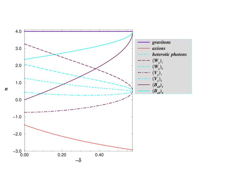
FIG. 1.: Spectral slopes for fluctuations that re-enter in the dual-dilaton phase when the latter is characterized by $\theta=1/\sqrt{3}$ (i.e. by constant moduli).

Consider now the energy stored in the amplified perturbations during the dual-dilaton phase. Figs. 1, 2 and 3 give the spectral slopes in various cases for the two relevant frequency ranges. Fig. 4 gives the normalization of the spectra in the whole frequency range for the particular case $\theta=1/\sqrt{3},\delta=-0.3$. Since all perturbations are of the same order at the maximal amplified frequency (here $f_{s}$), perturbations with (the most) negative spectral slope dominate over all others. From the above mentioned figures we see that the spectral slope of axionic fluctuations re-entering during the dual dilaton phase is generally the most negative one (at least if we consider isotropic compactifications): we thus ignore contributions to the energy density from perturbations other than the axion’s. The basic idea is to assume that the transition from the dual-dilaton phase to the radiation phase occurs precisely when the energy density in the perturbations becomes critical and starts to dominate over the kinetic energy of the coherent dilaton field.

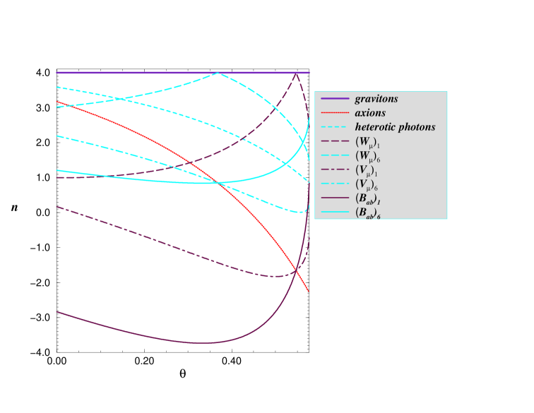
FIG. 2.: Same as Fig. 1 where, instead of fixing $\theta$, we fix $\delta=-0.26$ in the intermediate phase.

Let us fix for simplicity $\theta=1/\sqrt{3}$ (i.e. frozen internal dimensions in the dual-dilaton phase) and then impose criticality at the end of the dual-dilaton phase in the form:

$$M_{s}^{2}\,H_{1}^{2}\simeq e^{\varphi_{1}}\,\rho_{A}({\eta_{1}})\,.$$ (64)

Using the equations of motion and assuming $|\eta_{1}|\gg|\eta_{s}|$, we have

$$H_{1}\simeq M_{s}\,\left|\frac{\eta_{s}}{\eta_{1}}\right|^{(3+\sqrt{3})/2}\,,\quad\quad e^{\varphi_{1}}\simeq e^{\varphi_{s}}\,\left|\frac{\eta_{s}}{\eta_{1}}\right|^{-\sqrt{3}}\,.$$ (65)

Taking into account the results of Sec. IV we get, apart from factors $O(1)$,

$$\rho_{A}(\eta_{1}) \simeq f_{s}^{4}(\eta_{s})\,\left(\frac{a_{s}}{a_{1}}\right)^{4}\,\left(\frac{f_{1}}{f_{s}}\right)^{n_{A}}\simeq f_{s}^{4}(\eta_{s})\,\left|\frac{\eta_{s}}{\eta_{1}}\right|^{4/(1-\delta)}\quad,\,n_{A}<0\,,$$ (66)

where we have restricted ourselves to the case $n_{A}<0$ for the reasons explained above.

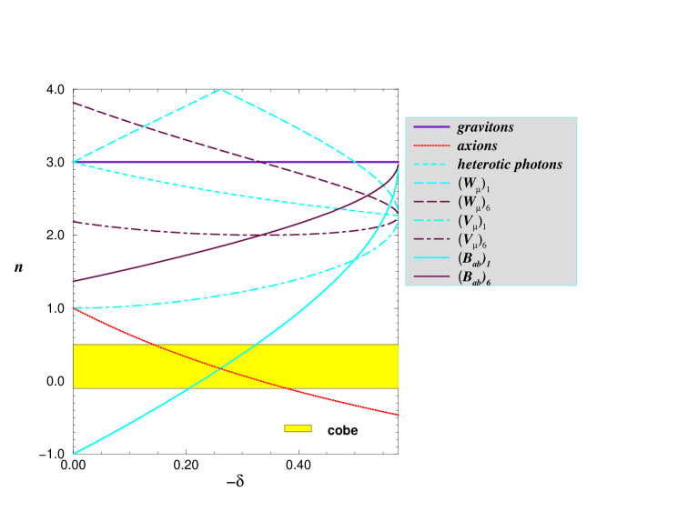
FIG. 3.: Spectral slopes for fluctuations that re-enter in the radiation phase. For comparison we also show the experimental constraint from COBE $[20]$: $n+1=1.2\pm 0.3$.

The dependence of the value of the dilaton background at $\eta=\eta_{1}$ on the parameter $\delta$ is completely fixed by the criticality condition Eq. (64). Indeed, inserting Eqs. (65) and (66) in Eq. (64), we obtain

$$e^{\varphi_{1}}\simeq\left|\frac{\eta_{s}}{\eta_{1}}\right|^{3+\sqrt{3}-4/(1-\delta)}\,.$$ (67)

If we define an effective temperature $T_{\rm eff}$ at the beginning of the radiation era by

$$\rho_{A}(\eta_{1})\simeq T_{\rm eff}^{4}\,,$$ (68)

we get

$$\left|\frac{\eta_{s}}{\eta_{1}}\right|\simeq\left(\frac{T_{\rm eff}}{M_{s}}\right)^{1-\delta}\,,$$ (69)

where we have assumed $f_{s}(\eta_{s})\sim M_{s}$, and thus

$$e^{\varphi_{1}}\simeq\left(\frac{T_{\rm eff}}{M_{s}}\right)^{(1-\delta)(3+\sqrt{3})-4}\,.$$ (70)

It is important to stress that this effective temperature may have nothing to do with the actual temperature of a relativistic gas in thermal equilibrium at $\eta=\eta_{1}$. In particular, if the coupling is still very small, axions may not thermalize at all, in spite of dominating the energy and of driving a radiation-dominated era. For the same reason, the fact that $T_{\rm eff}$ can be large in string units should not be a matter of concern.

Let us now estimate the value of the frequencies $f_{s}$ and $f_{1}$ at present time. If we assume that the CMB photons we observe today carry the (red-shifted) energy of the primordial perturbations (in particular from axion decay), we have

$$2\pi f_{1}=\frac{k_{1}}{a_{0}}\simeq\frac{a_{1}}{a_{0}}\,H_{1}\,,$$ (71)

$$\Omega_{\gamma}(t_{0})=\frac{1}{G(\eta_{1})M_{\rm Pl}^{2}}\,\frac{H_{1}^{2}}{H_{0}^{2}}\,\left(\frac{a_{1}}{a_{0}}\right)^{4}\,,$$ (72)

$$f_{1}^{4}\simeq G(\eta_{1})\,M_{\rm Pl}^{2}\,H_{0}^{2}\,H_{1}^{2}\,\Omega_{\gamma}(t_{0})\simeq e^{\varphi_{1}}\,H_{0}^{2}\,H_{1}^{2}\,\Omega_{\gamma}(t_{0})M_{\rm Pl}^{2}/M_{\rm s}^{2}\,,$$ (73)

where $H_{0}$ and $\Omega_{\gamma}(t_{0})$ ($\sim 10^{-4}$) are respectively the Hubble parameter and the fraction of the critical energy stored in radiation at the present time $t_{0}$. Using Eq. (65) and Eq. (69) we finally get

$$f_{1}\simeq\sqrt{H_{0}M_{\rm Pl}}\,e^{\varphi_{1}/4}\,(\Omega_{\gamma}(t_{0}))^{1/4}\,\left(\frac{T_{\rm eff}}{M_{s}}\right)^{(1-\delta)(3+\sqrt{3})/4}\,,$$ (74)

$$f_{s}\simeq f_{1}\,\left(\frac{T_{\rm eff}}{M_{s}}\right)^{\delta-1}\,.$$ (75)

Note that, if we choose $T_{\rm eff}=10^{15}\,{\rm GeV}$, corresponding to a relatively short dual-dilaton phase, and we fix $\delta=-0.3$ in order to have an almost flat axion spectrum in the low-frequency region (see Fig. 3), we get $f_{1}\sim 10^{5}\,{\rm Hz},f_{s}\sim 10^{9}\,{\rm Hz}$ and $\varphi_{s}\simeq-23,\varphi_{1}\simeq-11$. Therefore, the value of the dilaton at the beginning of the radiation era is still far from the present value ($\varphi_{0}\sim-1$).

Typical spectra for all the fields we have considered are shown in Fig 4. In particular, for axionic fluctuations that re-enter in the dual-dilaton phase ($f_{1}\ll f\ll f_{s}$), we get a decreasing spectrum

$$\Omega_{A}\simeq G(\eta_{1})\,H_{1}^{2}\,\Omega_{\gamma}(t_{0})\,\left(\frac{f}{f_{s}}\right)^{n_{A}}\,\left(\frac{f_{s}}{f_{1}}\right)^{4}\,.$$ (76)

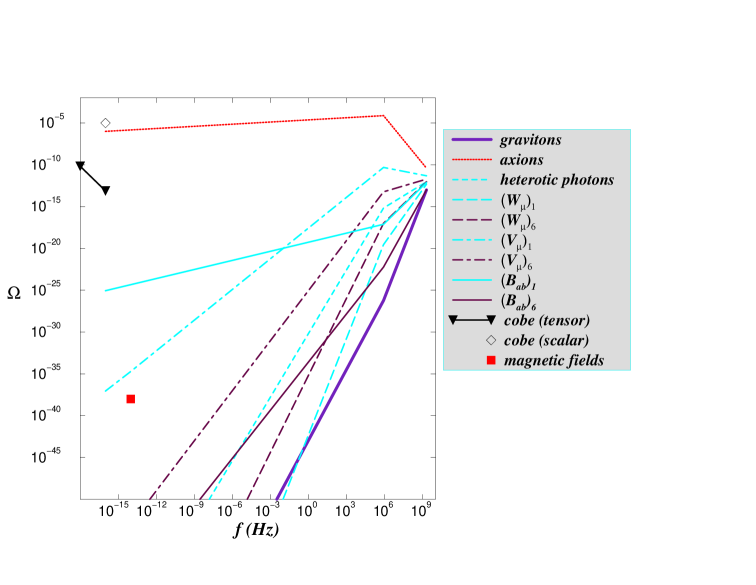
FIG. 4.: Spectrum for all the fluctuations considered in the case of a dual-dilaton intermediate phase, with the following choice: $\delta=-0.3$,   $\theta=1/\sqrt{3}$,   $f_{1}\sim 10^{5}\,{\rm Hz},f_{s}\sim 10^{9}\,{\rm Hz}$,  $\varphi_{s}\sim-23,\,\varphi_{1}\sim-11,$   $T_{\rm eff}=10^{15}\,{\rm GeV}$.

On the contrary, for fluctuations that re-enter in the radiation phase ($f\ll f_{1}\ll f_{s}$), we get

$$\Omega_{A} \simeq G(\eta_{1})\,H_{1}^{2}\,\Omega_{\gamma}(t_{0})\,\left(\frac{f}{f_{1}}\right)^{n_{A}}\,\left(\frac{f_{s}}{f_{1}}\right)^{2(\nu+\mu)}\,,$$ (77)

$$\simeq \Omega_{\gamma}(t_{0})\,\left(\frac{f}{f_{1}}\right)^{n_{A}}\,,$$ (78)

which includes the possibility of a scale-invariant flat spectrum.

As can be seen from Fig. 4, the Kaluza-Klein “photons” $V_{\mu}^{\,\,a}$, can give sufficiently large seeds for galactic magnetic fields ($\Omega>10^{-38}$ for $f_{M}\approx 10^{-14}$ Hz [19]) in this case, provided of course that the true electromagnetic field has a non-vanishing component along this direction in group space. Amusingly enough, this can be achieved in a range of moduli where axionic perturbations have a nearly flat spectrum.

B Intermediate string phase

In this scenario the Bogoliubov coefficients are still expressed by Eqs. (37), (39), (41) and (43), $\eta_{s}$ is the time at which the string phase starts, and we again assume that the radiation phase, dominated by the energy stored in the amplified vacuum fluctuations, begins at $\eta=\eta_{1}$. We recall that, in this case, $f_{1}>f_{s}$ and that we expect $f_{1}(\eta_{1})\sim M_{s}$. Since axions have the most negative spectral slope, we impose again that their energy density becomes critical at the beginning of the radiation phase:

$$H_{1}^{2}=G(\eta_{1})\,\rho_{A}(\eta_{1})\,,$$ (79)

Using then

$$\rho_{A}(\eta_{1})\simeq f_{1}^{4}(\eta_{1})\,\left(\frac{f_{s}}{f_{1}}\right)^{n_{A}}$$ (80)

and assuming again that the photons we observe today originate from the amplified vacuum fluctuations, we can fix the present value of $f_{1}$ to be

$$f_{1}(t_{0})\simeq\sqrt{H_{0}M_{\rm Pl}}\,e^{\varphi_{1}/4}\,(\Omega_{\gamma}(t_{0}))^{1/4}\,,$$ (81)

and relate $\varphi_{1}$ to the duration of the string phase $z_{s}=a_{1}/a_{s}$ (a free parameter)

$$e^{\varphi_{1}}\simeq z_{s}^{-2\zeta}\,.$$ (82)

If we define again

$$\rho_{A}(\eta_{1})\simeq T_{\rm eff}^{4}\,,$$ (83)

we obtain

$$z_{s}\simeq\left(\frac{T_{\rm eff}}{M_{s}}\right)^{2/\zeta}\,.$$ (84)

With the choice $T_{\rm eff}=2\times 10^{18}\,{\rm GeV},\zeta=0.08$, corresponding to a very long string phase, and fixing $\delta=-1/3$ in order to have a flat axion spectrum in the low-frequency region (see Fig. 3), we obtain

$$f_{1}\sim 10^{10}\,{\rm Hz},\,\,f_{s}\sim 8\cdot 10^{-1}\,{\rm Hz}\,\,,\varphi_{s}\simeq-8,\;\varphi_{1}\simeq-5\;.$$

As in the scenario with a dual-dilaton intermediate phase, we find the unpleasant result that the dilaton is still far from its present value at the beginning of the radiation era.

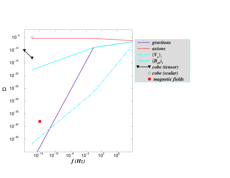
FIG. 5.: Some fluctuation spectra in the case of a string intermediate phase. The following choice of parameters was made: $\zeta=0.08$, $\delta=-1/3$, $f_{1}\sim 10^{10}\,{\rm Hz},f_{s}\sim 8\cdot 10^{-1}\,{\rm Hz}$, $\varphi_{s}\sim-8,\varphi_{1}\sim-5$,   $T_{\rm eff}=2\times 10^{18}\,{\rm GeV}$.

In Fig. 5 we summarize the results of the spectra for some perturbations. The spectrum of the fluctuations that exit in the dilaton phase is given in the limit $f\ll f_{s}\ll f_{1}$, using the coefficients ${\cal C}_{i}$, shown in Table I. For fluctuations that exit in the string phase we consider instead the limit $f_{s}\ll f\ll f_{1}$, and the Bogoliubov coefficients are expressed by the quantities ${\cal D}_{i}$ (see Table II after substituting $\gamma\rightarrow\kappa$ and $\kappa\rightarrow\alpha$).

Note that, for fluctuations of the axion field that exit in the string phase, we have

$$\Omega_{A} \simeq G(\eta_{1})\,H_{1}^{2}\,\Omega_{\gamma}(t_{0})\,\left(\frac{f}{f_{s}}\right)^{n_{A}}\,\left(\frac{f_{1}}{f_{s}}\right)^{2(\mu+\rho)-4}\,,$$ (85)

$$\simeq \Omega_{\gamma}(t_{0})\,\left(\frac{f}{f_{s}}\right)^{n_{A}}\,.$$ (86)

Substituting the parameters of Table I we get a decreasing spectrum

$$\Omega_{A}\simeq G(\eta_{1})\,H_{1}^{2}\,\Omega_{\gamma}(t_{0})\,\left(\frac{f}{f_{1}}\right)^{-2\zeta}\,.$$ (87)

In this example, a long string phase produces a gravitational spectrum of order $\sim 10^{-9}$ in the range of detection of LIGO/VIRGO, but a very steep spectrum of Kaluza-Klein photons $V_{\mu}^{\,\,a}$ at high frequencies and consequently a value of perturbations at $f_{M}\sim 10^{-14}\,{\rm Hz}$ far below the lower limit necessary to seed the dynamo mechanism for galactic magnetic fields [19].

VI Discussion

Our main results can be summarised as follows: Eqs. (55), (56), Tables III and  IV, Figs. 1, 2 and 3 give our main conclusions concerning the spectral slopes of the various spectra in the two scenarios, while Figs. 4 and 5 illustrate the spectra of all perturbations for certain typical choices of the background’s moduli. Rather than discussing the fine details, we would like to draw some conclusions, which appear to be relatively robust with respect to (slight?) variations of the moduli.

• Our calculations are based on the use of the low-energy effective action both for the backgrounds and for the perturbations. Since in the pre-big bang scenario a high-curvature phase is necessary before any exit to standard cosmology can be achieved, such a procedure is often criticized (see e.g. [21]) and requires some justification. We have seen in our explicit computations that the spectrum of long-wavelength perturbations, which exit and re-enter at small curvatures (in string units), does not depend on the details of the high curvature phase. Also, the use of higher-derivative-corrected perturbation equations has recently been shown [22] not to change the low-frequency spectra by more than a number $O(1)$. Thus predictions for the low-energy end of the spectra appear to be robust. Why? The physical explanation almost certainly lies in the freezing-out of super-horizon-scale perturbations. The occurrence of a constant mode at sufficiently large wavelengths can be shown without reference to the low-energy approximation [16] and, by a canonical transformation argument, should also apply to the constant-momentum mode. By contrast, the high frequency spectra are expected to depend quite crucially on the details of the strong curvature transition. We expect our naive formulae to give “lower bounds” for those parts of the spectra.

• The main result of our investigation is the confirmation of the suggestion found in ref.[15] that positive spectral slopes are by no means a must in pre-big bang cosmology. By computing the spectra after re-entry, we have confirmed that axions do have, more often than not, negative slopes (decreasing spectra). However, other fields, such as KK gauge fields and scalars, can also exhibit negative slopes. A particularly promising case is the one shown in Fig. 3, since, in a region around the one with nine-dimensional symmetry ($\delta=\pm\beta_{a}=-1/3$), the axion spectrum and that of a KK scalar field are nearly flat, while the slope of the spectrum of some KK gauge field is positive but sufficiently small to produce large enough seeds for the galactic magnetic fields.

• Unfortunately, the promising results of Fig. 3 are somewhat spoiled when a long dual-dilaton or string phase is inserted in the background between the dilaton and radiation phases. In this case, the spectral slopes grow somewhat wild in the negative direction (see e.g. Fig. 2 for the dual-dilaton case), making some of the spectra peak at very low frequency. The generic consequence of this phenomenon is a huge increase in the total, integrated energy density in the perturbations. If the string coupling (the dilaton) is not very small throughout the intermediate phase, the energy in these perturbations soon becomes critical and the intermediate phase stops. The only way to have a long intermediate phase is therefore to force the dilaton to be very perturbative until the end of the intermediate phase, be it the string or the dual-dilaton phase. In this case, however, at the beginning of the radiation phase the dilaton is still very much displaced from its present value (where supposedly the minimum of its non-perturbative potential is) and may have a hard time reaching it later. In other words, the most appealing possible scenarios appear to be those with a sudden transition between the dilaton and radiation phases occurring at “realistic” values for the string coupling (roughly $1/N$, if $N$ is the number of effectively amplified distinct species). Although this appears at present as some kind of fine tuning of the ratio of two moduli, it is not excluded that a better understanding of the initial conditions leading to PBB behaviour along the lines of Ref. [8] may tie together the initial values of the coupling and the curvature so that such conditions are naturally realised.

• If the latter picture is adopted, it is possible to have a nearly scale-invariant dilaton/moduli spectrum. This could lead to an interesting mechanism to generate large-scale anisotropy along the lines given in Ref.[14]. In the same region of moduli space one obtains reasonably large fluctuations of the KK gauge fields to provide sizeable seeds for the galactic magnetic fields. On the negative side, in this region of parameter space, the situation would be quite discouraging for generating a large enough gravitational-wave signal in the interesting frequency range.

Note added

While completing this work we became aware of a paper by Brustein and Hadad [23] which is also dealing with generic perturbations in string cosmology. Their method is somewhat different from ours: instead of working within a specific parametrization of the high-curvature phase, they have assumed the freezing of the fluctuation and of its conjugate momentum for super-horizon scales. Also, they have not imposed our criticality condition and thus have not obtained predictions on the value of the dilaton at the beginning of the radiation phase. We have checked that our results agree with theirs wherever a comparison is possible.

A

Here we give the explicit form of the coefficients entering the Bogoliubov formulae of Sec. IV C. In the case of the limit $f\ll f_{1}\ll f_{s}$ we get:

$${\cal N}_{1} = \frac{i}{8\pi}\,\frac{\Gamma(\mu)\,\Gamma(\nu)\,\Gamma(\rho)}{\Gamma(1+\mu)}\,,$$ (A1)

$${\cal C}_{1}^{1} = \left(\gamma-\kappa+\mu+\nu\right)\,\left(-\alpha+\kappa+\mu-\rho\right)\,,$$ (A2)

$${\cal C}_{1}^{2} = \left(\gamma-\kappa-\mu+\nu\right)\,\left(\alpha-\kappa+\mu+\rho\right)\,;$$ (A3)

$${\cal N}_{2} = -\frac{i}{8\pi}\,\frac{\Gamma(\mu)\,\Gamma(\nu)\,\Gamma(-\rho)}{\Gamma(1+\mu)}\,\left[\cos(\pi\,\rho)-i\,\sin(\pi\,\rho)\right]\,,$$ (A4)

$${\cal C}_{2}^{1} = \left(\gamma-\kappa+\mu+\nu\right)\,\left(\alpha-\kappa-\mu-\rho\right)\,,$$ (A5)

$${\cal C}_{2}^{2} = \left(\gamma-\kappa-\mu+\nu\right)\,\left(-\alpha+\kappa-\mu+\rho\right)\,;$$ (A6)

$${\cal N}_{3} = -\frac{i}{8\pi}\,\frac{\Gamma(\mu)\,\Gamma(-\nu)\,\Gamma(\rho)}{\Gamma(1+\mu)}\,\left[\cos(\pi\,\nu)-i\,\sin(\pi\,\nu)\right]\,,$$ (A7)

$${\cal C}_{3}^{1} = \left(\gamma-\kappa+\mu-\nu\right)\,\left(\alpha-\kappa-\mu+\rho\right)\,,$$ (A8)

$${\cal C}_{3}^{2} = \left(-\gamma+\kappa+\mu+\nu\right)\,\left(\alpha-\kappa+\mu+\rho\right)\,;$$ (A9)

$${\cal N}_{4} = -\frac{i}{8\pi}\,\frac{\Gamma(\mu)\,\Gamma(\nu)\,\Gamma(\rho)}{\Gamma(2-\mu)\,\Gamma(1+\mu)\,\Gamma(2+\mu)\,\Gamma(2-\nu)\,\Gamma(2-\rho)}\,,$$ (A10)

$${\cal C}_{4}^{1} = \left(\alpha-\kappa+\mu+\rho\right)\,\Gamma(2+\mu)\,\Gamma(2-\rho)\,\left[\left(-2+\gamma-\kappa-\mu+\nu\right)\right.$$ (A12)

$$\left.\,\Gamma(2-\mu)\,\Gamma(1-\nu)+\left(2+\gamma-\kappa-\mu+\nu\right)\,\Gamma(1-\mu)\,\Gamma(2-\nu)\right]\,,$$

$${\cal C}_{4}^{2} = \left(-\alpha+\kappa+\mu-\rho\right)\,\Gamma(2-\mu)\,\Gamma(2-\rho)\,\left[\left(-2+\gamma-\kappa+\mu+\nu\right)\right.$$ (A14)

$$\left.\,\Gamma(2+\mu)\,\Gamma(1-\nu)+\left(2+\gamma-\kappa+\mu+\nu\right)\,\Gamma(1+\mu)\,\Gamma(2-\nu)\right]\,,$$

$${\cal C}_{4}^{3} = \left(\gamma-\kappa+\mu+\nu\right)\,\Gamma(2+\mu)\,\Gamma(2-\nu)\,\left[\left(2-\alpha+\kappa+\mu-\rho\right)\,\right.$$ (A16)

$$\left.\Gamma(2-\mu)\,\Gamma(1-\rho)+\left(-2-\alpha+\kappa+\mu-\rho\right)\,\Gamma(1-\mu)\,\Gamma(2-\rho)\right]\,,$$

$${\cal C}_{4}^{4} = \left(\gamma-\kappa-\mu+\nu\right)\,\Gamma(2-\mu)\,\Gamma(2-\nu)\,\left[\left(-2+\alpha-\kappa+\mu+\rho\right)\right.$$ (A18)

$$\left.\Gamma(2+\mu)\,\Gamma(1-\rho)+\left(2+\alpha-\kappa+\mu+\rho\right)\,\Gamma(1+\mu)\,\Gamma(2-\rho)\right]\,;$$

while for fluctuations in the frequency region $f_{1}\ll f\ll f_{s}$ we obtain:

$${\cal D}_{1} = -\frac{i}{8}\,e^{-i\pi/2\,\left(-\mu+\rho\right)}\,\left(-\gamma+\kappa+\mu-\nu\right)\,\pi^{-1}\,2{\Gamma}(\mu)\,{\Gamma}(\nu)\,,$$ (A19)

$${\cal D}_{2} = -\frac{i}{8}\,e^{-i\pi/2\,\left(\mu+\rho\right)}\left(-\gamma+\kappa-\mu-\nu\right)\,\pi^{-1}\,2{\Gamma}(-\mu)\,{\Gamma}(\nu)\,,$$ (A20)

$${\cal D}_{3} = -\frac{i}{8}\,e^{-i\pi/2\,\left(2\nu-\mu+\rho\right)}\left(-\gamma+\kappa+\mu+\nu\right)\,\pi^{-1}\,2\Gamma(\mu)\,{\Gamma}(-\nu)\,,$$ (A21)

$${\cal D}_{4} = \frac{i}{8}\,e^{-i\pi/2\,\left(-\mu+\rho\right)}\,\pi\,\left[\left(2-\gamma+\kappa+\mu-\nu\right)\,(1-\mu)\,+\right.$$ (A23)

$$\left.\left(-2-\gamma+\kappa+\mu-\nu\right)\,(1-\nu)\right]\,\frac{2\Gamma(\mu)\,\Gamma(\nu)}{(1-\mu)\,(1-\nu)}\,.$$

REFERENCES

- [1] See, for instance, E.W.Kolb and M.S.Turner, The Early Universe (Addison-Wesley, Redwood City, 1990) and references therein.
-
[2]
G. Veneziano, Phys. Lett. B265, 287 (1991);
M. Gasperini and G. Veneziano, Astropart. Phys. 1 (1993) 317; Mod. Phys. Lett. A8 (1993) 3701; Phys. Rev. D50 (1994) 2519;
R. Brustein and G. Veneziano, Phys. Lett. B329 (1994)429;
N. Kaloper, R. Madden and K. A. Olive, Nucl. Phys. B452 (1995) 677; Phys. Lett. B371 (1996) 34;
R. Easther, K. Maeda and D. Wands, Phys. Rev. D53 (1996) 4247;
E. J. Copeland, A. Lahiri and D. Wands, Phys. Rev. D50 (1994) 4868, D51 (1995) 223;
J. D. Barrow and K. E. Kunze, Phys. Rev. D56 (1997) 741. - [3] A continuously updated collection of papers on the PBB scenario is available at http://www.to.infn.it/teorici/gasperini/.
- [4] M. Gasperini, M. Maggiore and G. Veneziano, Nucl. Phys. B494 (1997) 315.
- [5] R. Brustein and R. Madden, Graceful exit and energy conditions in string cosmology, BGU-PH-97/06 (hep-th/9702043); A model for graceful exit in string cosmology, BGU-PH-97/11 (hep-th/9708046).
-
[6]
G. Veneziano, ref. [2];
A.A. Tseytlin, Mod. Phys. Lett A6 (1991) 1721;
K.A. Meissner and G. Veneziano, Phys. Lett. B267 (1991) 33; Mod. Phys. Lett. A6 (1991) 3397;
A.A. Tseytlin and C. Vafa, Nucl. Phys. B372 (1992) 443.
A. Sen, Phys. Lett. B271 (1991) 295;
S.F. Hassan and A. Sen, Nucl. Phys. B375 (1992) 103;
M. Gasperini and G. Veneziano, Phys. Lett. B277 (1992) 256;
K.A. Meissner, Phys. Lett. B392 (1997) 298;
N. Kaloper and K.A. Meissner, Duality beyond the first loop, CERN-TH-97-113 (hep-th/9705193), to appear in Phys. Rev. D56. - [7] G. Veneziano, Phys. Lett. B406 (1997) 297.
- [8] A. Buonanno, K.A. Meissner, C. Ungarelli and G. Veneziano, Classical inhomogeneities in string cosmology, CERN-TH/97-124 (hep-th/9706221).
- [9] M.S. Turner and E.J. Weinberg, Phys. Rev. D56 (1997) 4604.
- [10] M. Maggiore and R. Sturani, The fine-tuning problem in pre-big bang inflation, IFUP-TH-22-97 (gr-qc/9706053).
-
[11]
R. Brustein, M. Gasperini, M. Giovannini and G.
Veneziano,
Phys. Lett. B361 (1995) 45;
R. Brustein, M. Gasperini and G. Veneziano, Phys. Rev. D55 (1997) 3882;
A. Buonanno, M. Maggiore, C. Ungarelli, Phys. Rev. D55 (1997) 3330;
B. Allen and R. Brustein, Phys. Rev. D55 (1997) 3260;
M. Gasperini, Phys. Rev. D56 (1997) 4815. - [12] R. Brustein, M. Gasperini, M. Giovannini, V.F. Mukhanov and G. Veneziano, Phys. Rev. D51 (1995) 6744.
-
[13]
M. Gasperini, M. Giovannini and G. Veneziano, Phys. Rev. Lett. 75
(1995) 3796;
D. Lemoine and M. Lemoine, Phys. Rev. D52 (1995) 1955. - [14] M. Gasperini, M. Giovannini and G. Veneziano, Phys. Rev. D52 (1995) 6651.
- [15] E. J. Copeland, R. Easther and D. Wands, Phys. Rev. D56 (1997) 874.
- [16] R. Brustein, M. Gasperini and G. Veneziano, to appear.
- [17] J. Maharana and J.H. Schwarz, Nucl. Phys. B390 (1993) 3.
- [18] M. Abramowicz and I. A. Stegun, Handbook of Mathematical Functions, (Dover, New York, 1972).
-
[19]
E. N. Parker, Cosmical magnetic fields,
(Clarendon Press, Oxford, 1979);
M.S. Turner and L.M. Widrow, Phys. Rev. D37 (1988) 2743. - [20] K.M. Gorski et al., Power spectrum of primordial inhomogeneity determined from the 4-year COBE DMR sky maps, COBE-PREPRINT-96-03 (astro-ph/9601063).
- [21] S.W. Hawking, talk presented at COSMO-97, Ambleside, England (September 1997).
- [22] M. Gasperini, ref. [11].
- [23] R. Brustein and M. Hadad, Particle production in string cosmology models, BGU-PH-97-12 (hep-th/9709022).