UNITU-THEP-20/1996 October 25, 1996
Monopoles and Strings in Yang-Mills Theories∗
K. Langfeld, H. Reinhardt, M. Quandt1
Institut für Theoretische Physik, Universität Tübingen
D–72076 Tübingen, Germany.
Abstract
Yang-Mills theory is studied in a variant of ’t Hooft’s maximal Abelian gauge. In this gauge magnetic monopoles arise in the Abelian magnetic field. We show, however, that the full (non-Abelian) magnetic field does not possess any monopoles, but rather strings of magnetic fluxes. We argue that these strings are the relevant infrared degrees of freedom. The properties of the magnetic strings which arise from a dilute instanton gas are investigated for the gauge group SU(2).
∗ Supported in part by DFG under contract Re 856/1-3.
1 Supported by Graduiertenkolleg ”Hadronen und Kerne”
1 Introduction
Confinement may be realized through a dual Meissner effect [1]. This confinement scenario assumes that the QCD ground state consists in a certain gauge of a condensate of magnetic monopoles. Such a dual super-conductor squeezes the color electric field between color charges into flux tubes and in this way provides confinement. This confinement scenario seems to be realized in super-symmetric models [2].
Although this idea dates back almost twenty years, recent developments in numerical simulations of lattice gauge theory provide the environment to test such ideas in a quantitative manner. The main ingredient in a derivation of the dual Meissner effect is the Abelian projection. Let us briefly illustrate this procedure for later use. The starting point is the Cartan decomposition of the gauge group where denotes the Cartan subgroup. Accordingly, the link variable is decomposed into an Abelian part and a coset part . The latter contains the gluonic field , which is charged with respect to the Cartan-group. Lattice calculations provide support for the notion that in the so-called maximal Abelian gauge [10], the Abelian field components and in particular the magnetic monopoles dominate the infrared physics (Abelian dominance) [4] and that those charged gluon fields which are assumed to be free of topological obstructions, can be perturbatively taken into account. In particular, for the tension of the string connecting static sources in the fundamental representation, the Abelian lattice configurations reproduce about 92% of the string tension and furthermore 95% of this part comes from the magnetic monopoles alone [5].
Despite the success at hand, recent studies cast doubt onto the widespread belief in Abelian dominance. From the analytical approach to finite temperature Yang-Mills theory of [6], supplemented by numerical results, the authors concluded that the Abelian projection provides correct qualitative features, whereas it fails at a quantitative level. To be more precise, lattice measurements reveal that the tension of the string between static sources of representation is proportional to the quadratic Casimir [7] (Casimir scaling). The Abelian dominance approximation obviously fails to reproduce this observation, since e.g. quarks in the adjoint representation possess Abelian charge zero, and hence the string tension in the Abelian approximation is zero in contradiction to the full lattice result [8]. This result indicates that the contributions of the charged fields to physical quantities are not negligible even in the infra red. This fact is confirmed by a large- analysis of SU(N) Yang-Mills theory [9]. It was observed that the forces between Abelian–charged and between Abelian–neutral sources possess the same order of magnitude. In this paper, we will provide further evidence that the charged gauge fields contribute to the partition function in a topological by non-trivial manner.
There is also evidence from other lattice calculations that the magnetic monopoles obtained in the maximal Abelian gauge need not be the most efficient infra red degrees of freedom. In the lattice study reported in [8], the Abelian gauge field is brought as close as possible to a gauge field by fixing the residual U(1) gauge symmetry. Assuming that this gauge field is the only relevant infra red degree of freedom (center dominance), the string tension of quarks in the fundamental representation111The center dominance approximation also fails to reproduce Casimir scaling [8]. was reproduced to high accuracy. This result suggests that the QCD vacuum is as well described in terms of vortices as by a condensate of monopoles.
In this paper we will show in a variant of ’t Hooft’s maximal Abelian gauge that the emergence of the magnetic monopoles is confined to the Abelian magnetic field , and therefore highly gauge dependent. We will find that the full (non-Abelian) magnetic field strength does not contain any monopoles. The Abelian magnetic monopole field is canceled by the commutator contribution to the field strength tensor. The full field strength, which is the relevant quantity in the partition function, possesses magnetic strings, which are the leftovers of the Dirac strings of the Abelian monopole field. We further argue that it is these strings rather than the magnetic monopoles which are the dominant infrared degrees of freedom. Finally, we discuss in detail the strings occurring in a dilute instanton medium.
The paper is organized as follows: in the next section, we will discuss the emergence of magnetic monopoles as artifacts of incomplete gauge fixings which leave a residual Abelian invariance. For a particular choice of the Abelian gauge fixing, we extract the magnetic string attached to the monopole. In section 3, we will show that the monopoles drop out from the full field strength while the string survives. We will argue that these strings are the relevant infra-red degrees of freedom. In section 4, the distribution of the string length will be investigated in a dilute instanton gas. Our conclusions will be left to the final section.
2 Topological Properties of monopoles
In what follows we briefly explain the emergence of magnetic monopoles in Abelian gauges and discuss their topological properties [1, 10]. We will find that the charges of these monopoles are quantized on topological grounds. Furthermore we will clarify in which respect these monopoles differ from the magnetic monopoles in classical electro dynamics.
Consider a field , which lives in the Lie algebra of the gauge group and transforms homogeneously under gauge transformations
| (1) |
We can fix the gauge by diagonalizing this field
| (2) |
where is a diagonal matrix with living in the Cartan sub-algebra. Mathematically, eq. (2) means that the field is conjugated into the maximal torus. Eq. (2) does not fix the gauge uniquely but still leaves invariance under transformations of the Cartan subgroup . Consequently the gauge function is defined only up to an element of the Cartan subgroup. In fact the transformation with does not change the field . Consequently the gauge transformation can be restricted to the coset space . At those points where two eigenvalues of coincide, the gauge function is not well defined. Without loss of generality we can arrange the eigenvalues of in such a way that the two degenerate eigenvalues correspond to a subgroup. In this case, it is obvious that these eigenvalues have to vanish at the degeneracy point . For simplicity let us confine ourselves in the following to the gauge group. Throughout this paper, we use anti-hermitian generators , where are the Pauli matrices. The gauge transformation which diagonalizes can be chosen as
| (3) |
where the unit color vector is given by
| (4) |
Then the degeneracy points correspond to vanishing field configurations . Near these degeneracy points the field hence has the form
| (5) |
with some constants . By a coordinate transformation , this configuration can be brought to the hedgehog form . As shown by ’t Hooft [1] (see also [10, 11]), the gauge transformation which diagonalizes the hedgehog field is such that the transformed gauge potential
| (6) |
develops a magnetic monopole at the degeneracy points .
Defining the Abelian magnetic field by
| (7) |
the magnetic flux through a closed surface is given by
| (8) | |||||
By Gauß’ theorem this flux vanishes since unless the gauge potential is singular somewhere on the surface . If the initial field configuration was smooth, then the first term in (6) will have no singularities. The magnetic monopole arises from the second term in (6) , and only this term contributes to the magnetic charge (8), which hence can be written as
| (9) |
For later convenience let us also introduce the normalized field defined by the unit vector in color space . Since this field defines a surface in color space. For given the field is well defined except at those points where the field (4) vanishes. We have therefore to exclude the position from the manifold on which is defined, i.e. the field is defined on the manifold , which is topologically equivalent to . Hence the chiral field defines a mapping from in coordinate space to the unit sphere in color space, defined by . Since such mappings fall into homotopy classes characterized by the winding number
| (10) |
where are coordinates of the in coordinate space and . In the gauge (2) this field has the representation
| (11) |
where . With this representation it is straightforward to show that the magnetic flux (9) divided by the volume of the unit sphere , , coincides with the winding number (10), i.e. . This implies that the magnetic charge of the monopole is quantized in integers. This result was already found in [10]. Note, however, that our definition of the magnetic charge differs from that in [10] by a factor of two.
Let us emphasize that the quantization of the magnetic monopoles arising in the Abelian gauge of non-Abelian gauge theories already occurs at classical level on purely topological grounds. This is different from the Dirac quantization of magnetic monopoles in QED. In the latter case, the quantization of magnetic charge results in the presence of an integer electric charge from the uniqueness of the wave function .
In order to calculate the magnetic charge (9), we have tacitly assumed that the gauge transformation is well defined in coordinate space except at the point . A glance at (4) shows that this is not the case, but is ill-defined along a string attached to the monopole, which is just the pendant of the Dirac string in classical electro dynamics222The above evaluation of the magnetic flux of the monopole assumes that the point where the string pierces the surface is excluded. Inclusion of this point would yield zero net magnetic flux out of the sphere, since the flux of the string is oppositely equal to the total flux of the magnetic monopole, see also below.. To be precise, the vector is singular for . Let us notice that this condition is in fact three constraints, which define the region in coordinate space where the gauge transformation (3) is not defined, i.e.
| (12) |
Whereas the first two equations generically select a line in space, the last condition of (12) chooses segments on this line. We therefore conclude that the regions where the gauge transformation (3) is ill-defined corresponds to strings which in most cases333Details will be presented in the next section. will have finite length. At the end-points of these strings, the equality holds in the last constraint of (12) implying that Abelian monopoles occur at the endpoints of the string. By performing an Abelian gauge transformation , the string can be arbitrarily deformed.
Let us illuminate the emergence of the string in more detail. For this purpose, we confine ourselves to the region of space close to the Abelian monopole. As discussed before, the gauge fixing field (5) then takes a hedgehog form. Without loss of generality, we may choose
| (13) |
where . In this case, the gauge transformation (3) is ill-defined on the negative -axis. In order to extract the -field configuration which is induced by the transformation (3), we regularize the induced gauge potential by
| (14) |
Introducing polar coordinates , the Abelian magnetic field (7) is given for any value of the regulator by
| (15) |
where , are the unit vectors in radial and -direction, respectively.


Removing the regulator in (15), one easily verifies by calculating the magnetic flux through the plane that the second term in (15) yields a -function for , i.e.
| (16) |
where is the step-function. The first term at the r.h.s. of (16) is precisely the Abelian monopole field. The second term represents the magnetic string lying on the negative -axis. From eq.(16), it is obvious that the magnetic flux of the monopole flowing out of the sphere equals the flux of the magnetic string flowing into the sphere.
3 Monopoles versus strings
As discussed above, in the gauge the Abelian magnetic field (7), arising from the induced gauge potential , develops a magnetic monopole at those points at which . In fact, we have seen that the employed gauge transformation is such that the quantity gives rise to a magnetic monopole field with a string attached. Contrary to classical electrodynamics, in the present case the string is not an artifact of a coordinate singularity but physically meaningful. Let us explain this fact in more detail.
In classical electrodynamics the primary quantity is the magnetic field of the monopole satisfying the equation
| (17) |
while the gauge potential itself has no physical meaning.
The (Dirac) string arises when one tries to represent the magnetic field of the monopole by a single overall defined gauge potential
| (18) |
In this case, since for any regular function, the gauge potential has to be singular in order to produce a magnetic monopole field (17), and the Dirac string arises. As we discussed in the previous section, the magnetic flux flowing through the Dirac string into the monopole is the same as the flux of the monopole field, and the monopole field together with the Dirac string gives rise to continuous magnetic flux lines, that is the total magnetic field of the monopole and the Dirac string is source, free . In this case, one has to exclude the magnetic field of the Dirac string in order to be left with the net magnetic monopole field satisfying (17). In this sense, the Dirac string is not a physical object in classical electrodynamics444In fact, the emergence of the Dirac string can be avoided by using the Wu-Yang construction, which employs different gauge potentials in the upper and lower hemispheres. In this case the gauge potential is discontinuous across the plane, and it is this discontinuity in the gauge potential which then provides the net magnetic flux of the monopole field. Note also that the Wu-Yang construction arises in a different gauge, namely . .
On the other hand, at quantum level the gauge potential itself becomes physically meaningful. It is this quantity which defines the quantum theory in both the operator and the functional integral approach. Furthermore, there are phenomena in topologically non-simply connected spaces, such as the Bohm-Aharonov effect, which cannot be exclusively described in terms of field strengths, but require resort to the gauge potential. Hence, in the quantum theory the string of the monopole field cannot be discarded.
Let us now consider the non-Abelian gauge theory and assume that we initially work in a gauge (e.g. ) in which all fields configurations are smooth. The magnetic monopoles here arise when we bring (originally smooth) gauge configurations into a particular (Abelian) gauge. By gauge invariance of the theory, the new gauge potential is equivalent to the smooth starting gauge potential and there is no reason why one should exclude parts of the gauge rotated potential . In particular, if the inhomogeneous part develops a magnetic monopole, there is no reason to exclude the corresponding string.
The string contributes to the Abelian magnetic flux (8) and cancels the contribution from the monopole (point) singularity as is easily checked by inserting (16) into (7,8).
Let us emphasize that the magnetic monopoles arise only in the Abelian magnetic field, which is induced by . At quantum level, there is a priori no reason to consider the Abelian magnetic field only. This is because the weight of a gauge potential in the partition function is determined by its full (non-Abelian) field strength. However, the induced gauge potential is a pure gauge in that region of coordinate space where is well defined. Consequently, its field strength
vanishes except at those points where is singular. Thus we expect a non-zero color-magnetic field only along the string singularity, and in the remaining part of the space the commutator term in the field strength has to compensate the Abelian magnetic field . This can be explicitly demonstrated by using the regularized gauge potential (14) of the monopole field and calculating the full (non-Abelian) magnetic field strength (3), see fig. 1. The monopole field has in fact disappeared, leaving only an extended string-like magnetic field. In the limit where the regulator is removed, one obtains a string of magnetic flux. Thus, instead of a gas of Abelian monopoles, we are left with an ensemble of strings.
Obviously, the magnetic strings transform homogeneously under regular gauge transformations. In this respect, the flux strings are more convenient variables than the monopole potentials. Lattice calculations have revealed that in the maximal Abelian gauge magnetic monopoles are the dominant infra red degrees of freedom at least for some observables, e.g. the tension of the chromo-electric string between quarks in the fundamental representation [4]. Since any magnetic monopole is connected to a string, we can alternatively consider these strings as the infra red dominant degrees of freedom. In fact, on a lattice magnetic monopoles are identified by measuring the magnetic flux of the corresponding string [12].
To summarize this section, we have shown that a string of magnetic field strength is attached to the monopoles in the Abelian magnetic fields which arise in Abelian gauges. In addition, one finds that the monopole field cancels in the full color-magnetic field, whereas the color-magnetic string survives. As long as we assume that in the quantum theory the gauge potential is the primary quantity (and not the field strength, as is argued in classical electro dynamics), the string must be regarded as an effective degree of freedom. Lattice theories which were designed to focus on the role of the Abelian monopoles by adopting proper gauges, have revealed that these monopoles play an important role for the confinement mechanism. Knowing about the intimate relation between the strings and the monopoles in particular Abelian gauges, it is tempting to assume that the magnetic strings are in fact the dominant infra red degrees of freedom. Thus, instead of a gas of monopoles, we are left with an ensemble of magnetic strings. To investigate the properties of such a string-dominated Yang-Mills vacuum as well as to study its impact for confinement is an interesting task for future work.
4 String statistics
From vortex condensation theory [13], we expect a non-trivial contribution of a string to the Wilson loop whenever the string pierces the loop area. It is therefore of particular interest to study the length distribution of the strings in the Yang-Mills vacuum. Since we do not know the field configurations which dominate the ground state, we must resort to a model description. At this stage of the investigation, we assume for simplicity that the Yang-Mills vacuum is given by a dilute instanton gas. In what follows, we will study the strings which arise by casting the instanton medium into an Abelian gauge.
In order to be specific, we choose the following gauge,
| (20) |
where is the squared field strength tensor evaluated with the gauge field configuration under consideration. Literally, eq. (20) is the time average of the zeroth component of the gauge potential, where acts as a measure for the averaging procedure. It is obvious that a time independent gauge transformation suffices to cast an arbitrary (time dependent) configuration into the gauge (20). Hence, the results of the previous sections apply also in the present case. Note that different powers of the field strength tensor in (20) are possible as well. Different choices correspond to different gauges.
The model configuration whose string content we wish to study here is a gas of (anti-) instantons, i.e.
| (21) |
where () is an orthogonal matrix which defines the orientation of the (anti-) instanton, and () is the position of the th (anti-) instanton. We have assumed that the instantons possess an unique radius , which is not an unrealistic assumption [15]. Note that the configuration (21) is an approximate solution of the Yang-Mills equation of motion if the instanton distances are large compared with . Here, we do not want to construct the lowest action solution which might serve as candidate for the (semi-classical) vacuum of Yang-Mills theory, but we would like to discuss the properties of the magnetic strings arising from a medium which is somewhat close to the (semi-classical) ground state.
For technical simplification, we approximate the total squared field strength in (20) by the superposition of the squared field strength of the single instantons, i.e.
| (22) |
Again, this approximation is justified, if the instanton gas is dilute. Alternatively, we can interpret the use of (22) in (20) as a change of the gauge choice.
For a single instanton, the magnetic monopole occurs at the instanton center, and the string extends from the center to infinity. Let us also briefly discuss the case of two instantons. For two widely separated instantons, the monopole position is given by the solution of the equation
| (23) |
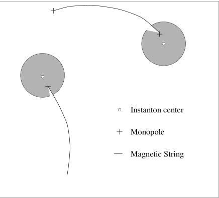
where is the functional (20) evaluated with the i-th instanton configuration. Since the contribution of , evaluated at the center of the first instanton, to the above equation is small, we expect a monopole occurring close to each instanton center. In addition, one finds a further monopole in between the two instantons. This additional monopole occurs, where both functions in (23) are small and cancel each other. Figure 2 qualitatively shows the behavior of the magnetic string, if two instantons are present. The generic picture for many instantons is that a string of finite length is attached to a point close to each instanton center.
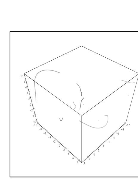
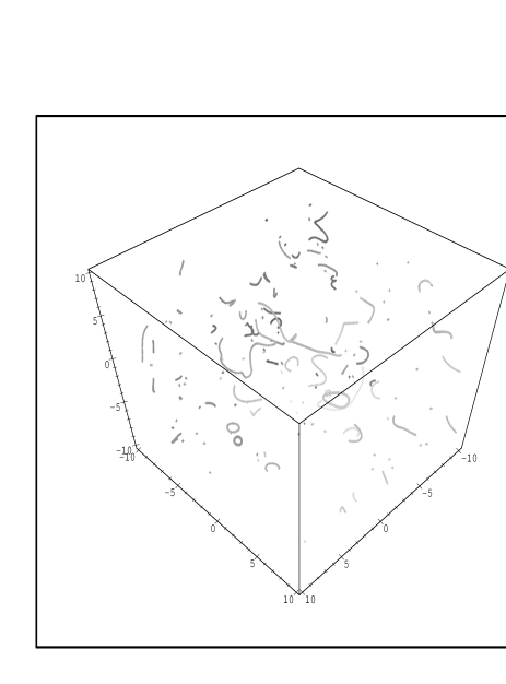
In order to be precise, we have calculated the positions of the strings arising from a multi-instanton medium, when the quantity (20) satisfies the conditions (12). Figure 3 shows the color-magnetic strings in coordinate space. The calculation was done for and instantons, and the positions and orientations of the instantons are chosen randomly. One observes that if the instanton density increases the length of the strings decreases.


By investigating several thousands of samples of strings inside the box, we extracted the string length distribution. The result is shown in figure 4. One observes a peak in the distribution at which is independent of the instanton density, whereas the bulk of the distribution strongly depends on number of instantons inside the box. The peak structure could arise from string configurations the length of which is determined by the properties of a single instanton rather than by the average instanton distance, e.g. by closed strings looping around the instanton center.

Finally, we present the relation between the string length and the inter-instanton distance (figure 5). At small densities (large ), the string length scales with the average distance between the instantons. If this average distance is smaller than a critical distance , the string length almost stays constant. A possible explanation is the following: at small instanton densities, the string length associated with a particular instanton is limited by the neighboring instanton. If the density increases, the strings start to percolate between the instantons, and therefore their lengths depend on the instanton radius rather than on . Although specific properties of string configurations might change, if the dilute gas approximation is abandoned, we do not expect significant changes in the gross features of the string distribution.
Let us comment on the physical implications of the string distribution. If a magnetic string pierces the minimal surface spanned by a Wilson loop, we expect a non-vanishing contribution to Wilson’s integral. The average length of the strings is therefore of crucial importance, since it determines the average number of strings piercing the surface. In a forthcoming publication, we will study the contribution of the strings to the Wilson loop in a quantitative manner.
5 Conclusions
We have studied the emergence of magnetic monopoles and strings in the Abelian projection (see e.g. [4]), which had been brought into question by recent papers [6, 8, 9]. We have argued that magnetic strings are the relevant infra red dominant degrees of freedom rather than monopoles. This conjecture is based on two observations: firstly, Abelian monopoles are an artifact in the sense that they always appear whenever a residual U(1) gauge degree of freedom remains unfixed. Secondly, magnetic strings rather than monopoles appear in the non-Abelian field strength. The monopole in the Abelian magnetic field, which stems from the neutral gauge field , is canceled in the full non-Abelian field strength by contributions from the charged fields . This implies that the charged gauge potentials carry as much topological information as the Abelian field .
The above conjecture received support from lattice calculations [8]. It was observed that the string tension can be reproduced by assuming a ”center dominance”. Within this approximation, the residual U(1) gauge-symmetry on the lattice is further reduced to a local symmetry, and the ground state of such a lattice model is known to be dominated by vortices rather than by monopoles.
In this paper, we did not further pursue the phenomenology of a string dominated ground state—this is left to a forthcoming publication—, but studied the properties of the strings which arise from a dilute instanton gas. Although this is not a very realistic model for the Yang-Mills vacuum [14], it should suffice to obtain first insights into string properties at least at finite temperatures. We found that the string length scales with the average instanton distance at small instanton densities, whereas the length depends only on the instanton radius at higher densities. An interesting issue for future investigations would be the identification of the strings on the lattice, and the study of their impact on confinement.
Acknowledgments:
We thank M. Engelhardt for useful comments on the manuscript.
References
- [1] G. ’t Hooft, High energy physics , Bologna 1976; S. Mandelstam, Phys. Rep. C23 (1976) 245; G. ’t Hooft, Nucl. Phys. B190 (1981) 455.
- [2] N. Seiberg and E. Witten, Nucl. Phys. B426 (1994) 19; Nucl. Phys. B431 (1994) 484.
- [3] For a review see e.g. T. Suzuki, Lattice 92, Amsterdam, Nucl. Phys. B30 (1993) 176, proceedings supplement.
- [4] M. N. Chernodub, M. I. Polikarpov, A. I. Veselov, Talk given at International Workshop on Nonperturbative Approaches to QCD, Trento, Italy, 10-29 Jul 1995. Published in Trento QCD Workshop 1995:81-91; M. I. Polikarpov, Talk given at Lattice 96, St. Louis, 1996, hep-lat/9609020.
- [5] G. S. Bali, V. Bornyakov, M. Mueller-Preussker, hep-lat/9603012, in press by Phys. Rev. D.
- [6] P. H. Damgaard, J. Greensite, M. Hasenbusch, Talk presented at Workshop on Nonperturbative Approaches to QCD, Trento, Italy, Jul 1995, hep-lat/9511007.
- [7] see e.g. M. Faber, H. Markum, Nucl. Phys. B26 (1988) 204, proceedings supplement.
- [8] D. Debbio, M. Faber, J. Greensite, S. Olejnik, Talk presented at Lattice 96, St. Louis, 1996, hep-lat/9607053.
- [9] D. Debbio, M. Faber, J. Greensite, Nucl. Phys. B414 (1994) 594.
- [10] A. S. Kronfeld, G. Schierholz, U.-J. Wiese, Nucl. Phys. B293 (1987) 461.
- [11] H. Suganuma, S. Sasaki, H. Toki, Nucl. Phys. B435 (1995) 207.
- [12] T. A. DeGrand, D. Toussaint, Phys. Rev. D22 (1980) 2478.
- [13] G. ’ Hooft, Nucl. Phys. B153 (1979) 141.
- [14] E. V. Shuryak, Nucl. Phys. B203 (1982) 93; Nucl. Phys. B302 (1988) 259; E. V. Shuryak, J. J. M. Verbaarschot, Nucl. Phys. B341 (1990) 1.
- [15] E. V. Shuryak, Phys. Rept. 115 (1984) 151.