QMW-93/15

hep-th/9307167

TOWARDS A STATISTICAL MECHANICS OF NONABELIAN VORTICES
CHINORAT KOBDAJ

and

STEVEN THOMAS

Department of Physics
Queen Mary and Westfield College
Mile End Road
London E1
U.K.
ABSTRACT

A detailed study is presented of classical field configurations describing nonabelian vortices in two spatial dimensions, when a global $SO(3)$ symmetry is spontaneously broken to a discrete group ${\rm I\kern-1.79993ptK}$ isomorphic to the group of integers mod 4. The vortices in this model are characterized by the nonabelian fundamental group $\pi_{1}(SO(3)/{{\rm I\kern-1.79993ptK}})\cong\hbox{$\,\vrule height=6.45831pt,width=0.4pt,depth=0.0pt\kern-3.00003pt{\rm Q}$}_{8}$, which is isomorphic to the group of quaternions. We present an ansatz describing isolated vortices in this system and prove that it is stable to perturbations. Kinematic constraints are derived which imply that at a finite temperature, only two species of vortices are stable to decay, due to ‘dissociation’. The latter process is the nonabelian analogue of the well known instability of charge $|q|>1$ abelian vortices to dissociation into those with charge $|q|=1$. The energy of configurations containing at maximum two vortex-antivortex pairs, is then computed. When the pairs are all of the same type, we find the usual Coulombic interaction energy as in the abelian case. When they are different, one finds novel interactions which are a departure from Coulomb like behavior. These results allow one to compute the grand canonical partition function (GCPF) for thermal pair creation of nonabelian vortices, in the approximation where the fugacities for vortices of each type are small. It is found that the vortex fugacities depend on a real continuous parameter $a$ which characterize the degeneracy of the vacuum in the model considered. Depending on the relative sizes of these fugacities, the vortex gas will be dominated by one of either of the two types mentioned above. In these regimes, we expect the standard Kosterlitz-Thouless phase transitions to occur, as in systems of abelian vortices in 2-dimensions. Between these two regimes, the gas contains pairs of both types, so nonabelian effects will be important. The results presented should provide a starting point from which to investigate screening properties of the nonabelian vortex gas.

1 Introduction

The study of vortex defects in both two and three spatial dimensions, has revealed many interesting properties which have had a wide variety of applications in both condensed matter physics [1], and cosmology [2]. In their guise as cosmic strings [1], vortices in three spatial dimensions, which occur as the result of the spontaneous breakdown of a global symmetry in the early universe, may go some way in explaining the origin of large scale structure. At the other extreme, it has been known for some time [3] that vortices in 3-dimensional condensed systems such as superfluid helium IV, play an important role in understanding the properties of these systems.

It is well known that vortex defects in any dimension are characterized by $\pi_{1}(M)$, the fundamental group of the vacuum manifold $M$ of the theory. The type of vortex defects that occur in for example helium IV are ‘abelian’ in the sense that they are characterized (as we shall review later), by an abelian fundamental group, isomorphic to the group of integers ZZ. In 2-spatial dimensions, abelian vortices have particularly simple interactions which allows one to write down the grand canonical partition function (GCPF) for thermal pair creation to all orders in the vortex fugacity in terms of the so called Coulomb gas model [4]. The pioneering work of Berezinski [5], and Kosterlitz and Thouless [6], into their statistical mechanical properties, showed that a gas of such vortices underwent a novel kind of phase transition at some critical temperature ${\rm T}_{\rm c}$. A simple physical picture emerged where for T $<{\rm T}_{\rm c}$, vortices and antivortices form a medium of bound pairs which subsequentally dissociates into free vortices and antivortices for T $>{\rm T}_{\rm c}$. These results when applied to approximately 2-dimensional systems such as helium IV thin films, lead Kosterlitz and Nelson [7] to predict a universal jump in the superfluid density at ${\rm T}_{\rm c}$, which was later experimentally verified [8].

In this paper we shall study some properties of nonabelian vortices in two spatial dimensions, which should eventually lead to an understanding of their statistical mechanical properties. There is particular interest in these kind of vortex systems, not only because they are interesting extensions of those described above, but also because they are known to occur in certain 2-dimensional liquid crystals [9]. In fact, we shall consider the simplest model of spontaneous global symmetry breaking that yields a nonabelian $\pi_{1}(M)\cong\hbox{$\,\vrule height=6.45831pt,width=0.4pt,depth=0.0pt\kern-3.00003pt{\rm Q}$}_{8}$ where the latter is the order 8 group associated with the field of quaternions. Vortices described by this fundamental group are just those which are expected to occur in so called nematic liquid crystals [9]. As we shall see in later sections, the interactions of nonabelian vortices are very much more complicated than their abelian counterparts, so much so that we cannot expect to be able to write down the complete nonabelian vortex gas partition function to all orders in the relevant fugacities. We will only calculate the latter to fourth order in fugacities. Whilst this may seem very far from the all orders results in the abelian case, it is still sufficient to investigate whether a kind of nonabelian charge screening occurs, as we shall now explain.

Ordinary abelian charge screening is the mechanism behind the Kosterlitz-Thouless type phase transition described above [1]. There are a number of ways of exhibiting this screening, for example by exploiting the map between the vortex gas partition function and that of sine-Gordon theory in 2-dimensions [10]. Alternatively one may derive a so called Poisson-Boltzmann (P-B) equation [11], satisfied by the linearly screened potential between a test vortex and antivortex placed in the gas. The latter equation is derived in a perturbative small fugacity expansion, and it is clear that in order to compute the first order screening effects one needs to know the energy of a configuration with at least two vortices and two antivortices. One of these vortex-antivortex pairs will play the role of test charges, whilst the other will describe lowest order screening due to thermal pair creation. Of course due to the abelian properties, the resulting P-B equation is relatively simple as are its solutions [1]. One learns however, that it is not necessary to have an exact expression for the partition function, to investigate screening properties.

From the results given in this paper, it should be possible to generalize the notion of linearly screened potential, and to derive a nonabelian version of the Poisson-Boltzmann equation [12].

The structure of the paper is as follows. In Section 2 we introduce the 2-dimensional field theory model which describes nonabelian vortices associated with $\pi_{1}(M)\cong\hbox{$\,\vrule height=6.45831pt,width=0.4pt,depth=0.0pt\kern-3.00003pt{\rm Q}$}_{8}$. After a brief review of the homotopic classification of vortices, we present an ansatz describing isolated nonabelian vortices, and give numerical minimum energy solutions for the Higgs fields that define their ‘core’ region. The properties of these solutions are shown to guarantee finite energy. In Section 3 we present an ansatz for multivortex configurations and write down an expression for the GCPF describing the thermal creation of vortex-antivortex pairs. The energy density of all relevant configurations up to a maximum of four vortices is calculated. Section 4 describes a method for obtaining the explicit form of the total energy of each of these configurations. As an illustrative example, the method is used to compute the energy of a particular configuration in which nonabelian effects are expected to be important. After a conclusion and comment on the results, Appendix A gives details of a proof that our ansatz for isolated nonabelian vortices is indeed one of minimum energy. We should say at this point that there have been a number of recent papers concerning the subject of nonabelian vortices (e.g. ref.[13]). However these differ from our approach in that the symmetry breaking leading to nonabelian vortices is local. Moreover, the main investigations of these papers concerns the quantum properties of nonabelian vortices and their connections to systems obeying fractional spin statistics.

2 Definition of the model

In this section we shall describe in detail, a Higgs system which will give rise to nonabelian vortices based on the discrete group ${\hbox{$\,\vrule height=6.45831pt,width=0.4pt,depth=0.0pt\kern-3.00003pt{\rm Q}$}}_{8}$ of quaternions. As stated previously, the latter are probably the simplest examples of nonabelian vortices, but which also have direct physical interest. We shall consider the Higgs model first described in [14], where the scalar field or order parameter $\Phi$ is in the five dimensional representation of $SO(3)$ , and so can be written as a traceless, symmetric $3\times 3$ matrix. The energy density of the model is taken to be

$${\cal E}={1\over 2}{\rm Tr}\ \,\Bigl{[}g^{ab}\,\left(\partial_{a}\Phi\right)\left(\partial_{b}\Phi\right)\Bigr{]}-\,V(\Phi)$$ (2.1)

where the potential is chosen to be

$$V(\Phi)\ =\ {\lambda\over 4}\,\rm Tr\,\Phi^{4}+{\lambda^{\prime}\over 4}(\,\rm Tr\,\Phi^{2})^{2}+{\rho\over 3}\,\rm Tr\,\Phi^{3}-{1\over 2}\mu_{0}^{2}\,\rm Tr\,\Phi^{2}$$ (2.2)

and $g_{ab}$ is the 2-dimensional flat euclidean metric, where $a,\,b\,=\,1,\,2$ run over 2-dimensional polar coordinates (r, $\theta$ ) respectively.

Any field configuration $\Phi$ can be diagonalized by some orthogonal transformation $A$

$$A\,\Phi\,A^{T}\equiv\,\Phi_{diag}=\,{\rm diag}(\varphi_{1},\varphi_{2},-\varphi_{1}-\varphi_{2}).$$ (2.3)

Since $V(\Phi)$ is $SO(3)$ invariant, we have

$$V(\Phi) \ =\ V(A\,\Phi\,A^{-1})\ =\ V(\varphi_{1},\varphi_{2})$$ (2.4)

$$\ =\ {\lambda\over 4}(\varphi_{1}^{4}+\varphi_{2}^{4}+(\varphi_{1}+\varphi_{2})^{4})+{\rho\over 3}(\varphi_{1}^{3}+\varphi_{2}^{3}-(\varphi_{1}+\varphi_{2})^{3})$$

$$- {1\over 2}\mu_{0}^{2}(\varphi_{1}^{2}+\varphi_{2}^{2}+(\varphi_{1}+\varphi_{2})^{2})+{\lambda^{\prime}\over 4}[(\varphi_{1}^{2}+\varphi_{2}^{2}+(\varphi_{1}+\varphi_{2})^{2})]^{2}$$

The extrema of the potential, are given by the solution to the equations

$$0 \ =\ \lambda(2\varphi_{1}^{3}+\varphi_{2}^{3}+3\varphi_{1}^{2}\varphi_{2}+3\varphi_{1}\varphi_{2}^{2})+\rho(-\varphi_{2}^{2}-2\varphi_{1}\varphi_{2})$$

$$- \mu_{0}^{2}(2\varphi_{1}+\varphi_{2})+\lambda^{\prime}(4\varphi_{1}^{3}+2\varphi_{2}^{3}+6\varphi_{1}^{2}\varphi_{2}+6\varphi_{1}\varphi_{2}^{2})$$

$$0 \ =\ \lambda(2\varphi_{2}^{3}+\varphi_{1}^{3}+3\varphi_{1}^{2}\varphi_{2}+3\varphi_{1}\varphi_{2}^{2})+\rho(-\varphi_{1}^{2}-2\varphi_{1}\varphi_{2})$$

$$- \mu_{0}^{2}(\varphi_{1}+2\varphi_{2})+\lambda^{\prime}(2\varphi_{1}^{3}+4\varphi_{2}^{3}+6\varphi_{1}^{2}\varphi_{2}+6\varphi_{1}\varphi_{2}^{2})$$

Writing $\varphi_{2}=a\,\varphi_{1}\,$for some real parameter $a$, we have to solve two simultaneous cubic equations (2), (2) in say the variable $\varphi_{1}$. For $\rho=0$, but arbitrary $\lambda,\,\lambda^{\prime}$ one finds that there are degenerate set of minima which lie on an ellipse in the $\varphi_{1}-\varphi_{2}$ plane, defined by the equation

$$[(\lambda+\lambda^{\prime})\,(\,\varphi_{1}^{2}+\,\varphi_{1}\,\varphi_{2}+\,\varphi_{2}^{2})\,-\,1]=0$$ (2.7)

where in eqn.(2.7), and in the rest of the paper, we absorb the mass scale $\mu_{0}$ into the fields $\varphi_{1},\ \varphi_{2}$. For varying values of $\lambda$ and $\lambda^{\prime}$, eqn.(2.7) defines a continuum set of ellipses, illustrated in Fig.1 . If $\rho\neq 0$, then in fact this degeneracy is broken to a large extent, and the potential has three absolute minima at the points $\varphi_{2}=\,a\,\varphi_{1}$ on the same ellipses, with $a=1,\,-1/2$ and $-2$ respectively. These minima are indicated by the intersection of the three dashed radial lines with the ellipses in Fig.1. Since the vacuum expectation value $<\Phi>$ can be written in terms of $\varphi_{1}$ and $a$ at a minimum, one has

$$<\Phi>=\varphi_{1}\pmatrix{1&0&0\cr 0&a&0\cr 0&0&-1-a\cr}$$ (2.8)

It is clear from eqn.(2.8) that when $\rho\neq 0$, the three absolute minima correspond to an unbroken $U(1)$ global symmetry, when $<\Phi>$ is invariant under rotations about the $x,\,y$ and $z$-axes , for $a=1,\,-1/2$ and $-2$ respectively. When $\rho=0$ there is again an unbroken $U(1)$ at the above three points as well as at three new points corresponding to the intersection of the ellipse with the dotted radial lines in Fig.1. The dotted lines shown in this figure are just the continuation through the origin of the dashed radial lines, which together define the lines $\varphi_{2}=a\,\varphi_{1}$ for the three values of $a$ just given. For $\rho\neq 0$, the vacuum manifold $M$, i.e., the set of points in the space of matrices given by $\Phi={\cal G}<\Phi>{\cal G}^{-1}$, ${\cal G}\,\in\,SO(3)$ , will be given by the quotient space $M$ = $SO(3)$/$U(1)$. The fundamental group of $M$ in this case will be isomorphic to $\mathchoice{\hbox{\cmss Z\kern-3.99994ptZ}}{\hbox{\cmss Z\kern-3.99994ptZ}}{\lower 0.9pt\hbox{\cmsss Z\kern-2.79996ptZ}}{\lower 1.2pt\hbox{\cmsss Z\kern-2.79996ptZ}}_{2}$, the group of integers modulo 2. As such, the vortices which can arise after this symmetry breaking will necessarily be abelian in nature. Since we wish to investigate vortices of the nonabelian variety in this paper, we shall take the coupling $\rho$ always to be zero. Then as long as we choose values for $<\varphi_{1}>$ and $<\varphi_{2}>$ on the ellipse which do not coincide with the six points at which $U(1)$ symmetry remains unbroken, the maximum symmetry group of $<\Phi>$ will be a discrete subgroup ${\rm I\kern-1.79993ptK}$ of $SO(3)$, which is isomorphic to the group of integers mod 4. As we shall see in more detail below, this leads to the manifold $M$ having a fundamental group given by the nonabelian discrete group ${\hbox{$\,\vrule height=6.45831pt,width=0.4pt,depth=0.0pt\kern-3.00003pt{\rm Q}$}}_{8}$, isomorphic to the group of quaternions. Throughout the rest of this paper, we shall concentrate on this case.

We now move on to discuss in detail an ansatz for isolated nonabelian vortices with specific reference to the group ${\hbox{$\,\vrule height=6.45831pt,width=0.4pt,depth=0.0pt\kern-3.00003pt{\rm Q}$}}_{8}$. In appendix A we shall show that our ansatz is the correct one in that it describes vortices with the lowest energy. The vacuum manifold for the case when $<\Phi>$ breaks $SO(3)$ down to the discrete subgroup ${\rm I\kern-1.79993ptK}$ which has elements

$${\cal K}_{1} = \pmatrix{1&0&0\cr 0&1&0\cr 0&0&1\cr}\qquad{\cal K}_{2}=\pmatrix{-1&0&0\cr 0&-1&0\cr 0&0&1\cr}$$

$${\cal K}_{3} = \pmatrix{-1&0&0\cr 0&1&0\cr 0&0&-1\cr}\qquad{\cal K}_{4}=\pmatrix{1&0&0\cr 0&-1&0\cr 0&0&-1\cr}$$ (2.9)

is given by $M=\ SO(3)/{\rm I\kern-1.79993ptK}\cong SU(2)/\hbox{$\,\vrule height=6.45831pt,width=0.4pt,depth=0.0pt\kern-3.00003pt{\rm Q}$}_{8}$, where we have used the well known homomorphism between $SO(3)$ and $SU(2)$. It follows that vortices are characterized by $\pi_{1}(M)\cong\hbox{$\,\vrule height=6.45831pt,width=0.4pt,depth=0.0pt\kern-3.00003pt{\rm Q}$}_{8}$. Using the homomorphism between $SO(3)$ and $SU(2)$ we can equally work with fields $\Phi$ which are representations of either group. We will usually work with $SO(3)$ representations and group elements (the latter denoted by $\cal{G}$ ) but will often give the corresponding $SU(2)$ fields and elements (denoted by $g$ ), on which $\hbox{$\,\vrule height=6.45831pt,width=0.4pt,depth=0.0pt\kern-3.00003pt{\rm Q}$}_{8}$ has a simple action.

Our ansatz for a single vortex at the origin in the $(r,\theta)$ plane will be

$$\Phi(r,\theta)\ =\ {\cal G}(\theta)\,\Phi_{diag}(r)\,\,{\cal G}^{-1}(\theta)$$ (2.10)

where in eqn.(2.10), $\Phi_{diag}$ denotes the diagonal matrix ($\varphi_{1}(r),\varphi_{2}(r),-(\varphi_{1}(r)+\varphi_{2}(r))$ ). It is assumed that $\varphi_{1},\varphi_{2}$ are functions of $r$ only whilst the group elements $\cal{G}$ depend only on $\theta$. It is important that on encircling the vortex at $r=0$, i.e. as $\theta$ is varied from 0 to 2$\pi$, $\Phi(r,\theta)$ be strictly single-valued. The corresponding boundary conditions on $\cal{G}(\theta)$ consistent with this constraint are,

$${\cal G}(\theta+2\,\pi)\,=\,{\cal G}(\theta)\,h$$ (2.11)

where h is an element of ${\rm I\kern-1.79993ptK}$. It might appear that there are only four ‘types’ of vortices corresponding to the four elements of ${\rm I\kern-1.79993ptK}$. However it should be remembered that $SO(3)$ is not simply connected since $\pi_{1}(SO(3))\cong\mathchoice{\hbox{\cmss Z\kern-3.99994ptZ}}{\hbox{\cmss Z\kern-3.99994ptZ}}{\lower 0.9pt\hbox{\cmsss Z\kern-2.79996ptZ}}{\lower 1.2pt\hbox{\cmsss Z\kern-2.79996ptZ}}_{2}$, which effectively doubles the number of homotopically inequivalent closed curves on $M$. This is more transparent when working with $SU(2)$ group elements. Under the homomorphism $SU(2)\cong SO(3)$, the group of quaternions $\hbox{$\,\vrule height=6.45831pt,width=0.4pt,depth=0.0pt\kern-3.00003pt{\rm Q}$}_{8}$ gets mapped to the abelian group ${\rm I\kern-1.79993ptK}$. So somewhat hidden in the boundary conditions given in eqn.(2.11) is the fact that closed curves on $M$ are actually characterized by elements of $\hbox{$\,\vrule height=6.45831pt,width=0.4pt,depth=0.0pt\kern-3.00003pt{\rm Q}$}_{8}$.

Next we need find out what are the explicit representations of $\pi_{1}(M)$. From a mathematical point of view there are of course, an infinite number of homotopically equivalent representations. However, we are only interested in the physically relevant ones, i.e. those which yield a minimum energy for the corresponding vortex, and we expect that such ‘minimal’ representations will be unique. The elements ${\cal K}_{2},...,{\cal K}_{4}$ given in eqn.(2) correspond to discrete rotations by 180 degrees about the $x,y$ and $z$-axes respectively. Therefore, a simple ansatz for the $SO(3)$ elements $\cal{G}$ which satisfy the boundary conditions in eqn.(2.11) for a given element of ${\rm I\kern-1.79993ptK}$, is for them to be rotations by angles $\theta/2$ about the respective axes. In fact, we shall show in Appendix A that this ansatz actually corresponds to minimal energy vortices.

In Table 1, we have listed these elements, together with the corresponding $SU(2)$ representations. Also listed are the discrete group elements that appear in the boundary conditions as we encircle the vortex. The $SU(2)$ representations in particular, make it clear that this group is $\hbox{$\,\vrule height=6.45831pt,width=0.4pt,depth=0.0pt\kern-3.00003pt{\rm Q}$}_{8}$. We have used the notation ${\cal G}_{i},{\cal G}_{j},{\cal G}_{k}$, ${\cal G}_{i}^{-1},{\cal G}_{j}^{-1},{\cal G}_{k}^{-1}$ and ${\cal G}_{-{\rm 1\kern-2.31001pt1}}$ to denote group elements whose boundary conditions are twisted by the elements $i,j,k,-i,-j,-k$ and -11 of $\hbox{$\,\vrule height=6.45831pt,width=0.4pt,depth=0.0pt\kern-3.00003pt{\rm Q}$}_{8}$, where

$${i}^{2}={j}^{2}={k}^{2}=-{\rm 1\kern-3.30002pt1}$$

$$i\,j\,=\,k\quad,\quad j\,k\,=\,i\quad,\quad k\,i\,=\,j$$ (2.12)

are the multiplication rules of $\hbox{$\,\vrule height=6.45831pt,width=0.4pt,depth=0.0pt\kern-3.00003pt{\rm Q}$}_{8}$. The parameter ${\theta}_{0}$ in Table 1 is an arbitrary constant associated with the origin of the $\theta$ coordinate.

Given these explicit forms for ${\cal G}$, we want to minimize the energy in eqn.(2.1) in the remaining fields $\varphi_{1}(r),\varphi_{2}(r)$, in order to find stable vortex solutions. Because of the $\Phi\rightarrow-\Phi$ symmetry of the energy, (assuming $\rho=0$ ), the equations for minimizing the energy will be the same for ${\cal G}_{\alpha}$ as for ${\cal G}_{\alpha}^{-1}$, for $\alpha\ \epsilon\ {\hbox{$\,\vrule height=6.45831pt,width=0.4pt,depth=0.0pt\kern-3.00003pt{\rm Q}$}}_{8}$. We shall refer to these as being vortices and antivortices of type $\alpha$ respectively. Furthermore, the vortices of type -11 are by nature abelian since -11 commutes with all other elements in $\hbox{$\,\vrule height=6.45831pt,width=0.4pt,depth=0.0pt\kern-3.00003pt{\rm Q}$}_{8}$. Moreover, we shall see in the next section that in a finite temperature system they are unstable to dissociation into either $i,j$ or $k$ type vortex-antivortex pairs. For these reasons we will concentrate for the remainder of the paper, on vortices of type $i,j$ and $k$. The parameter $\alpha$ which denotes species type, will therefore implicitly run over only these particular types.

Substituting the ansatz for ${\cal G}_{k}$ in these three cases into the energy we get

$$E_{\alpha} = \int d^{2}x\ \Biggl{\{}{1\over 2}{\rm Tr}\ \,\Biggl{[}\,g^{ab}\,\left(\partial_{a}\Phi\right)\left(\partial_{b}\Phi\right)\Biggr{]}-\,V\Biggr{\}}$$ (2.13)

$$= \int_{0}^{\infty}dr\,r\int_{0}^{2\pi}d\theta\ \,\Biggl{\{}{1\over 2}(\partial_{r}\varphi_{1})^{2}+{1\over 2}(\partial_{r}\varphi_{2})^{2}+{1\over 2}(\partial_{r}(\varphi_{1}+\varphi_{2}))^{2}$$

$$\qquad+\ {1\over{2\,r^{2}}}\,{P}_{\alpha}(\varphi_{1},\varphi_{2})-V(\varphi_{1},\varphi_{2})\Biggr{\}}$$

The effect of the terms ${\cal G}_{\alpha}(\theta)$ on the energy ${E}_{\alpha}$ is to add certain potential terms, denoted by ${1\over{r^{2}}}\,{P}_{\alpha}(\varphi_{1},\varphi_{2})$ in eqn.(2.13 ) which are given by

$${P}_{i}\ =\ {1\over 2}\,(\varphi_{1}\,+\,2\,\varphi_{2})^{2}$$ (2.14)

$${P}_{j}\ =\ {1\over 2}\,(2\,\varphi_{1}\,+\,\varphi_{2})^{2}$$ (2.15)

$${P}_{k}\ =\ {1\over 2}\,(\,\varphi_{1}\,-\,\varphi_{2})^{2}$$ (2.16)

The minimization equations for ${E}_{\alpha}$ are

$${2\partial_{rr}\varphi_{1}+{2\over r}\,\partial_{r}\varphi_{1}}+\partial_{rr}\varphi_{2}+{1\over r}\partial_{r}\varphi_{2}-{1\over{2\,r^{2}}}\frac{\partial{P}_{\alpha}}{\partial\varphi_{1}}+\frac{\partial V}{\partial\varphi_{1}} = 0$$

$${2\partial_{rr}\varphi_{2}+{2\over r}\,\partial_{r}\varphi_{2}}+\partial_{rr}\varphi_{1}+{1\over r}\partial_{r}\varphi_{1}-{1\over{2\,r^{2}}}\frac{\partial{P}_{\alpha}}{\partial\varphi_{2}}+\frac{\partial V}{\partial\varphi_{2}} = 0$$ (2.17)

On physical grounds, (namely the finiteness of the core energy ${E}_{\alpha}^{c}$, which we will be defined later), we anticipate that the solutions to these equations that minimize the energy have the following asymptotic behavior in the radial coordinate $r$. As $r\rightarrow 0$, it is sufficient that $\varphi_{1}$ and $\varphi_{2}$ both vanish at least as fast as $r$, whilst for $r\rightarrow\infty$, we expect both $\varphi_{1}$ and $\varphi_{2}$ go to their vacuum values, which minimize $V$. To show that smooth interpolating functions exist with these asymptotic properties, one may solve the non-linear differential equations (2) numerically. This was done by discretizing the energy in eqn.(2.1) and carrying out numerical minimization, for various values of the parameters $\lambda,\lambda^{\prime}$ and vacuum parameter $a$. Fig.2. illustrates the solutions found in the case of an $i$-type vortex with $\lambda=0.01$ and 2, $\lambda^{\prime}=0$ and $a=-1$ (we shall explain why we are interested in the value $a$ = -1 later). In Fig.2, the dotted curves show the numerical solutions whilst the solid ones are those of a trial solution, needed as input in the minimization procedure. These trial solutions are of the form

$$\varphi_{1}|_{trial} = \frac{1}{\sqrt{\lambda(1+a+a^{2})}}\left(\frac{r\mu_{0}}{r\mu_{0}+1}\right)$$

$$\varphi_{2}|_{trial} = \frac{a}{\sqrt{\lambda(1+a+a^{2})}}\left(\frac{r\mu_{0}}{r\mu_{0}+1}\right)$$ (2.18)

The normalization factors in eqns.(2) are such that $\varphi_{1}(\infty),\varphi_{2}(\infty)$ lie on the ellipse of degenerate vacua, described in the previous section.

As one can verify from Fig.2, these trial solutions are very good approximations, particularly close to the origin of $r$. It is also apparent that there is a ‘core’ region (marked as $r$ = ${r}_{c}$ in Fig.2) beyond which the values of $\varphi_{1},\varphi_{2}$ do not change appreciably, from their vacuum values . Of course, different definitions of $r_{c}$ are possible, depending on how close to unity one requires the ratios $\varphi_{1}/<\varphi_{1}>$ and $\varphi_{2}/<\varphi_{2}>$ to be. The lack of a precise core radius is not a particular property of nonabelian vortices, but is also apparent in the abelian case. What is clear in both cases however, is that different choices for $r_{c}$ will simply give rise to constant factors in the expression for the self energy of a vortex (see eqn.(2.19) below). Similar solutions to these exist for $j$ and $k$ type vortices, the only difference is in the algebraic form of the potentials ${P}_{\alpha}$ which, it turns out, has a minimal effect on the behaviour of the solutions. It will be a very useful (and good) approximation to replace the numerical solutions for $\varphi_{1},\varphi_{2}$ of $i,\,j$ and $k$ type vortices by those of the trial solutions given in eqns.(2) for the region $r\leq{r}_{c}$, and by $<\varphi_{1}>,<\varphi_{2}>$ for $r>{r}_{c}$.

This being the case, it is straight forward to compute the energy of a single $i,\ j$ or $k$ type vortex (or antivortex), placed in a 2-dimensional circular box of radius $R$. The result is

$${E}_{\alpha}\ =\ {E}_{\alpha}^{c}+\pi\,<{P}_{\alpha}>{{\rm ln}}\,\left({R\over{{r}_{c}}}\right)\quad\quad\alpha={i,j,k}$$ (2.19)

where ${r}_{c}$ is the core radius of the corresponding vortex configuration, and is typically of order unity in units of inverse mass ${\mu}_{0}^{-1}$. The logarithmic self energy terms in eqn.(2.19), correspond to contributions coming from the region $r>{r}_{c}$. The core energy, ${E}_{\alpha}^{c}$ in eqn.(2.19) can be approximated by taking the range of integration in eqn.(2.13) to be between $r=0$ and $r={r}_{c}$, and is given by

$${E}_{\alpha}^{c} = \pi\,<{P}_{\alpha}>\int_{0}^{r_{c}}\frac{{\rm d}r}{r}\left(\frac{r}{r+1}\right)^{2}\,+\,f(<\varphi_{1}>,<\varphi_{2}>,r_{c})$$ (2.20)

$$= \pi\,<{P}_{\alpha}>\{{{\rm ln}}\,(r_{c}+1)+\frac{1}{r_{c}+1}-1\}\,+\,f(<\varphi_{1}>,<\varphi_{2}>,r_{c})$$

The first term in eqn.(2.20) comes from the potential $P_{\alpha}$ present in $E_{\alpha}$ due to vortices of type $\alpha$. The second term $f(<\varphi_{1}>,<\varphi_{2}>,r_{c})$ represents contributions coming from other terms in (2.13), which are independent of the vortex type $\alpha$. These can be easily calculated, but explicit expressions will not be needed in what follows. It is worth comparing the results of eqns.(2.19), (2.20) to those one would obtain for a single abelian vortex in 2-dimensions, such as those produced in spontaneous breaking of $U(1)$ symmetry [15]. In the abelian case we would also obtain an energy formula similar to eqn.(2.19), with the coefficient of the logarithm term proportional to $q^{2}\,<\phi^{2}>$, where $q$ is the vorticity and $<\phi>$ is the $U(1)$ breaking vacuum expectation value. Hence the factors of $<{P}_{\alpha}>$ in eqn.(2.19), (2.20) for fixed $<\varphi_{1}>$ and $<\varphi_{2}>$ are proportional to a kind of nonabelian vorticity or nonabelian charge. The difference between the abelian and nonabelian example is that in the former, we can have arbitrarily large (but quantized) vorticity $q$, whilst in the latter there are clearly only a finite number of possibilities, given by the range of $\alpha$. This is a consequence of ${\pi}_{1}(M)\cong\mathchoice{\hbox{\cmss Z\kern-3.99994ptZ}}{\hbox{\cmss Z\kern-3.99994ptZ}}{\lower 0.9pt\hbox{\cmsss Z\kern-2.79996ptZ}}{\lower 1.2pt\hbox{\cmsss Z\kern-2.79996ptZ}}$, ( ZZ being the group of integers), and ${\pi}_{1}(M)\cong{\hbox{$\,\vrule height=6.45831pt,width=0.4pt,depth=0.0pt\kern-3.00003pt{\rm Q}$}}_{8}$ in the abelian and nonabelian cases respectively.

Finally, we can understand the logarithmic behavior in eqn.(2.20) and in particular why there is a logarithmic divergence as $R\rightarrow\infty$, even for nonabelian vortices. This is because, as the numerical results suggest, one can think of these vortices as having a definite core region, which for distances $r\gg{r}_{c}$, appears approximately as a point-like charge. It is natural then that the field energy outside such an isolated point charge be divergent as we go to the infinite volume limit, whilst the logarithmic behaviour is simply a consequence of the 2-dimensionality of the system. In fact, to see the truly novel effects of nonabelian vortices we have to study more than simply self-energies. Clearly we have to consider multi-vortex configurations where at least two of the vortices are of types h and g where the latter are two non-commuting elements of $\hbox{$\,\vrule height=6.45831pt,width=0.4pt,depth=0.0pt\kern-3.00003pt{\rm Q}$}_{8}$. We shall study this situation in the next section .

3 Systems of multi-vortices

Having discussed at length in the previous section the ansatz corresponding to isolated nonabelian vortices we now move on to discuss multiple vortex configurations. The simplest such configuration would be a vortex-antivortex pair of type $\alpha$. Since we are ultimately interested in the statistical mechanical properties of such vortices, one should consider what happens in a real system at finite temperature. The logarithmically divergent self energy of a single vortex discussed in the last section, prohibits, in the thermodynamic limit, single vortex creation in these systems due to thermal fluctuations. This is a property which is familiar in the case of abelian vortices [1]. However, neutral vortex-antivortex pair creation is not suppressed in this way, and one should therefore expect these to be present at finite temperature.

Intuitively we expect that whatever the correct description of such a pair is, it should go over to the previous ansatzes for an isolated vortex and antivortex in the limit where we take the distance between the pair very large with respect to their typical core size $r_{c}$. As such we shall take as our ansatz for a vortex of type $\alpha$ at the point $z_{1}$ and an antivortex of the same type at $z_{2}$ to be

$${\cal G}_{\alpha}(z,z_{1},z_{2})\simeq{\cal G}_{\alpha}(z,z_{1}){\cal G}_{-\alpha}(z,z_{2})$$ (3.1)

where in eqn.(3.1), the ${\cal G}_{\alpha}$ correspond to the 1-vortex solutions obtained in the previous section. The corresponding field configuration denoted by $\Phi_{\alpha}$ is

$$\Phi_{\alpha}\,=\,{\cal G}_{\alpha}(z,z_{1})\,{\cal G}_{\alpha}^{-1}(z,z_{2})\Phi_{diag}(z,z_{1},z_{2})\,{\cal G}_{\alpha}(z,z_{2})\,{\cal G}_{\alpha}^{-1}(z,z_{1})$$ (3.2)

Again, for well separated pairs we expect that the ‘core’ field $\Phi_{diag}$ vanishes as $z$ approaches either of the vortex centre’s at $z_{1}$ or $z_{2}$ , (which ensures a finite core energy in each case) just as in the 1-vortex case. In fact this behavior can be confirmed if one were to solve the minimum energy equations for $\varphi_{1},\varphi_{2}$ for the vortex pair with ${\cal G}_{\alpha}$ given by eqn.(3.2). As $z$ approaches either of $z_{1}$ or $z_{2}$, the form of ${\cal G}_{\alpha}$ goes over to that of the single vortex, modulo an unimportant constant shift in the angular coordinate $\theta$. Hence from our results of the last section, it is clear that the solutions for $\varphi_{1},\varphi_{2}$ will become, in the limit of large pair separation, those described in the previous section. Thus as before we can approximate $\varphi_{1},\varphi_{2}$ to be given by their vacuum values at distances $|z-z_{s}|\geq r_{c}$, where $s$ = 1, 2 . For distances $|z-z_{s}|<r_{c}$ we can approximate the fields by the trial solutions given in eqn.(2). Putting all this together we find that the energy of a vortex-antivortex pair is given by

$$E_{\alpha}(z_{1},z_{2})\,=\,2E_{\alpha}^{c}+2E_{\alpha}^{self}+E_{\alpha}^{int}(z_{1},z_{2})$$ (3.3)

where in eqn.(3.3) the core energy $E_{\alpha}^{c}$ was given in (2.20). The self energy $E_{\alpha}^{self}$ and interaction energy $E_{\alpha}^{int}$ are computed to be

$$E_{\alpha}^{self} = \pi\,<{P}_{\alpha}>{\rm ln}({R\over{r_{c}}})$$

$$E_{\alpha}^{int}(z_{1},z_{2}) = 2\,\pi\,<{P}_{\alpha}>{\rm ln}|\frac{z_{1}-z_{2}}{R}|$$ (3.4)

where $R$ is the size of the system, and the functions ${P}_{\alpha}$ were defined in eqns.(2.14)-(2.17). Note that we can take the thermodynamic limit $R\rightarrow\infty$ in eqn.(3 ) since $R$ cancels between the self and interaction energies. This is simply a consequence of taking a vortex -antivortex pair-which can be thought of as neutral. This phenomenon is already known to occur in the case of abelian vortices, and indeed $E_{\alpha}^{int}(z_{1},z_{2})$ above, is just the standard Coulomb type of interaction which one also finds in this case. This is not surprising because simply studying a vortex-antivortex pair of type $\alpha$ does not probe the nonabelian structure of the theory since ${\cal G}_{\alpha}$ and ${\cal G}_{-\alpha}$ are commuting elements. Clearly to study the effects due to non-commuting elements ${\cal G}_{\alpha},{\cal G}_{\beta}$, we have to look at least to configurations containing four vortices: a vortex-antivortex pair of type $\alpha$ interacting with a pair of different type $\beta$.

Before studying the details of this, we can make life easier by consideration of what one might call kinematical constraints associated with the thermal creation of vortices. As we shall see this implies that for any given value of the vacuum parameter $a$, only two types of vortices will be stable to dissociation into one another, where these types depend on the specific value of $a$.

Let us imagine creating vortex-antivortex pairs in a system by gradually increasing the temperature. The self energy eqn.(3) of a vortex of type $\alpha$ in the pair is proportional to the quantity $<P_{\alpha}>$ (see eqn.(3). As we discussed earlier, the $<P_{\alpha}>$ factors can be thought of as being proportional to a generalization of vortex charge or vorticity to the nonabelian case. As such one has to consider whether a nonabelian vortex of given charge is unstable to ‘splitting’ into two other vortices in such a way as to conserve overall charge, yet lower the self energy.

To understand this process let us consider the abelian case once more. Here the vortex self energies are proportional to $q^{2}$ , where $q$ is the quantized vortex charge. Thus it is clear that a charge $q$ = $\pm$2 vortex will be unstable to dissociation into two charge $\pm 1$ vortices because $E_{q={\pm 2}}^{self}>2E_{q={\pm 1}}^{self}$. The same is true for all higher charged abelian vortices with $|q|>1$, so that in this sense $|q|=1$ vortices are ultimately stable [15]. This explains why only $q$ = 1 vortices are considered in the context of Coulomb gas models and K-T type phase transitions [1]. We want to apply a similar analysis in the nonabelian case. The main differences are that we have a finite number of possible charges in this case as explained earlier, and the rules for possible dissociation of vortices are governed by the group relations of $\hbox{$\,\vrule height=6.45831pt,width=0.4pt,depth=0.0pt\kern-3.00003pt{\rm Q}$}_{8}$ not simply by the addition of charges.

It should be stressed at this point that the stability to dissociation we are discussing is different to, and must be considered in addition to, the perturbative stability analysis performed in Appendix A. Clearly the process of dissociation of a vortex is non-local, and is separate from the stability of a vortex to local perturbations.

To begin with consider the self energy of a -11 type vortex. We saw in the previous section that there were three kinds of ansatz for the $SO(3)$ element, denoted by ${\cal G}_{-{\rm 1\kern-2.31001pt1}}^{(\zeta)}$, where $\zeta$ runs over the elements $i,j,k$ of $\hbox{$\,\vrule height=6.45831pt,width=0.4pt,depth=0.0pt\kern-3.00003pt{\rm Q}$}_{8}$ (see Table 1). It is easy to see that the corresponding self energies $E_{-{\rm 1\kern-2.31001pt1}}^{self,(\zeta)}$satisfy the relations

$$E_{-{\rm 1\kern-2.31001pt1}}^{self,(\zeta)}\,=\,4E_{\zeta}^{self}>2E_{\zeta}^{self}$$ (3.5)

for arbitrary values of $a$. It is clear that -11 type vortices are always unstable to dissociation into a pair of vortices of type $i,j$ or $k$. Which actual decay branch occurs depends on the specific value of $a$ and will be whatever is the lowest energy of the three possibilities $E_{-{\rm 1\kern-2.31001pt1}}^{self,(\zeta)}$. From a practical point of view however, this result means that we need not consider -11 type vortices at all in investigating the statistical mechanics of nonabelian vortices. They are like the $|q|>1$ abelian vortices referred to above. Let us now consider the remaining cases of type $\alpha$ (clearly since $E_{\alpha}^{self}=E_{-\alpha}^{self}$ the arguments will hold equally for antivortices ).

Using the group composition rules for $\hbox{$\,\vrule height=6.45831pt,width=0.4pt,depth=0.0pt\kern-3.00003pt{\rm Q}$}_{8}$, a $k$ type vortex for example, can dissociate into an $i$ and $j$ type (or -$i$ and -$j$ type ) if

$$E_{k}^{self}\, > \,E_{i}^{self}+E_{j}^{self}$$ (3.6)

$$\Rightarrow {(1-a)}^{2}\,>\,{(1+2a)}^{2}+{(a+2)}^{2}\qquad{\rm i.e.}-2\,<\,a\,<-\frac{1}{2}$$

where in eqn.(3.6), we have substituted for $\varphi_{2}$ in terms of the parameter $a$. Thus in the interval $-2<a<-1/2$ , referred to as region ${\rm{\bf I}}_{ij}$ in Fig.3 , $k$ -type vortices dissociate, and at most we would expect to just find vortices and antivortices of type $i$ and $j$ in this region. At the same time we learn that $i$ and $j$ -type are stable to further dissociation, since in either case the path (restricted by the composition rules of $\hbox{$\,\vrule height=6.45831pt,width=0.4pt,depth=0.0pt\kern-3.00003pt{\rm Q}$}_{8}$), necessarily involves producing a $k$ type vortex. Notice that while ${\rm{\bf I}}_{ij}$ is a connected portion of the real line of $a$ values, the corresponding regions in the space of vacuum expectation values $<\varphi_{1}>,<\varphi_{2}>$ are two disconnected pieces. A similar analysis of possible decays of $i$ and $j$ types for $a$ values outside of region ${\rm{\bf I}}_{ij}$ gives the following results,

$$E_{i}^{self}\, > \,E_{j}^{self}+E_{k}^{self}$$ (3.7)

$$\Rightarrow \,\,{(1+2a)}^{2}\,>\,{(2+a)}^{2}+{(1-a)}^{2}\qquad{\rm i.e.}\,\,a\,<\,-2\ {\rm or}\ a\,>\,1$$

and finally

$$E_{j}^{self}\, > \,E_{k}^{self}+E_{i}^{self}$$ (3.8)

$$\Rightarrow \ {(2+a)}^{2}\,>\,{(1+2\,a)}^{2}+{(1-a)}^{2}\qquad{\rm i.e.}\,-\frac{1}{2}<a<1$$

the different regions of $a$ given in eqns.(3.7, 3.8 ) are denoted by ${\rm{\bf I}}_{jk}$ and ${\rm{\bf I}}_{ki}$ in Fig.3. Fig.3 clearly shows that the three regions fit together exactly, to cover the entire ellipse of vacuum states, without overlap. This means that the two types of vortices indicated by the subscripts on ${\rm{\bf I}}_{ij},{\rm{\bf I}}_{jk}$ and ${\rm{\bf I}}_{ki}$ are stable to further dissociation. It is interesting to see that all regions are separated by points with either $a=-1/2,1$ or $2$, which correspond to an unbroken $U(1)$ symmetry (see Section 2 ). At such points there are no vortices, so it appears that one cannot smoothly go from one region to another by varying $a$. In fact the relative positions of the regions ${\rm{\bf I}}_{ij},{\rm{\bf I}}_{jk}$ and ${\rm{\bf I}}_{ki}$ in Fig.1. can be understood in the following way.

The point where any two regions touch has an unbroken $U(1)$ symmetry that correspond to rotations about either the $x,y$ or $z$ axis, depending on which of the six points, where regions ${\rm{\bf I}}_{ij}$ etc meet, we consider. For example at the point where ${\rm{\bf I}}_{ij}$ and ${\rm{\bf I}}_{jk}$ meet, the $U(1)$ symmetry corresponds to rotations about the $y$-axis (which one can easily see from the form of $<\Phi>$ (see eqn.(2.8)) at this point). In some sense, we can now understand why this particular symmetry should appear here because in ‘passing’ from ${\rm{\bf I}}_{ij}$ to ${\rm{\bf I}}_{jk}$, the vortices of type $i$ have been rotated by 180 degrees about the $y$-axes into those of type $k$ whilst leaving those of type $j$ invariant. The other regions in Fig.3, and their relation to the particular $U(1)$ symmetry present at their intercept, can be similarly understood.

The end result of the above kinematic considerations, is that for any given ratio $<\varphi_{2}>/<\varphi_{1}>=a$, we need only concern ourselves with the statistical mechanics of two species of vortices. Let us for definiteness choose $a$ to be in the region $-2<a<-1/2$, i.e. we only study $i$ and $j$ type vortices.

Within this approximation, we can write down a general expression for the grand canonical partition function (GCPF) $Z$ of thermal pair creation of the above species of nonabelian vortices,

$$Z({\sl z}_{i},{\sl z}_{j})\, = \,\mathop{\sum}_{{N}_{i}=0}^{\infty}\mathop{\sum}_{{N}_{j}=0}^{\infty}\,\frac{{{\sl z}_{i}}^{N_{i}}}{{N_{i}!}}\,\frac{{{\sl z}_{j}}^{N_{j}}}{{N_{j}!}}\mathop{\prod}_{{\nu}_{i}=1}^{N_{i}}\mathop{\prod}_{{\nu}_{j}=1}^{N_{j}}\mathop{\int}\frac{{\rm d}^{2}{z_{{\nu}_{i}}}}{\pi{r_{c}}^{2}}\mathop{\int}\frac{{\rm d}^{2}{z_{{\nu}_{j}}}}{\pi{r_{c}}^{2}}$$ (3.9)

$$\times \sum_{\scriptstyle\left\{{\cal G}_{{\nu}_{i}}\right\}\,\atop\scriptstyle\,{\scriptstyle\prod\atop\scriptstyle{{\nu}_{i}}}{\cal G}_{{\nu}_{i}}={{\rm 1\kern-2.31001pt1}}}\,\sum_{\scriptstyle\left\{{\cal G}_{{\nu}_{j}}\right\}\,\atop\scriptstyle\,{\scriptstyle\prod\atop\scriptstyle{{\nu}_{j}}}{\cal G}_{{\nu}_{j}}={{\rm 1\kern-2.31001pt1}}}\,{\rm exp}\left\{-\frac{1}{\rm T}{\rm E}(N_{i},N_{j},{\cal G}_{{\nu}_{i}},{\cal G}_{{\nu}_{j}},z_{{\nu}_{i}},z_{{\nu}_{j}})\right\}$$

In eqn.(3.9 ), the fugacities ${\sl z}_{i},{\sl z}_{j}$ associated with vortices of type $i$ and $j$, are defined in terms of the core energies ${E}_{\alpha}^{c}$ given in eqn.(2.20)

$${}{\sl z}_{i} = {\rm exp}(-E_{i}^{c}/{\rm T}))$$

$${\sl z}_{j} = {\rm exp}(-E_{j}^{c}/{\rm T})$$ (3.10)

respectively. ${\cal G}_{{\nu}_{i}}$ and ${\cal G}_{{\nu}_{j}}$ denote the $SO(3)$ group elements corresponding to all the $i$ and $j$ type vortices of a particular configuration having total energy $E$. As we have already seen in this section, only configurations with ${\mathop{\prod}_{{\nu}_{i}=1}^{N_{i}}{\cal G}_{{\nu}_{i}}={{\rm 1\kern-3.30002pt1}}}$ and ${\mathop{\prod}_{{\nu}_{j}}^{N_{j}}{\cal G}_{{\nu}_{j}}={{\rm 1\kern-3.30002pt1}}}$ will contribute to the GCPF above, in the thermodynamic limit. Although eqn.(3.9) is a complete formula for the GCPF, we want to study it perturbatively in a small ${\sl z}_{i}$ and ${\sl z}_{j}$ expansion since we do not know how to compute $E$ for arbitrary configurations of $i$ and $j$ type vortices.

Having considered in some detail the case of single vortex -antivortex pairs, we now move on to consider the next order terms (in a double expansion of $Z$ in the fugacities ${\sl z}_{i},{\sl z}_{j}$ ). These will be configurations containing four vortices and antivortices arranged in two pairs, because the overall neutrality condition mentioned previously, demands that we consider only even numbers of vortices and antivortices. The simplest configuration of this type consists of two vortex-antivortex pairs of the same type $i$ or $j$. Because the pairs are of the same type, they commute with each other, so we expect that the resulting energy be that of the corresponding Coulomb system of charges [1,4]. The ansatz for this system will be just the generalization of the single pair ansatz given in eqn.(3.1), which again we expect to be a reasonable approximation at inter-pair distances greater than the core size $r_{c}$. Thus with the understanding that the index $\alpha$ now runs over $i$ and $j$ types only, the $SO(3)$ group element, ${\cal G}_{\alpha,\alpha}$, corresponding to vortices of type $\alpha$ at points $z_{1}$ and $z_{3}$ and antivortices of the same type at $z_{2},z_{4}$ will be

$${\cal G}_{\alpha,\alpha}(z_{1},\cdots,z_{4})\simeq{\cal G}_{\alpha}(z,z_{1})\,{\cal G}_{\alpha}(z,z_{2})\,{\cal G}_{\alpha}(z,z_{3})\,{\cal G}_{\alpha}(z,z_{4})$$ (3.11)

with the corresponding form of $\Phi$, which we denote by ${\Phi}_{\alpha,\alpha}$ being

$$\Phi_{\alpha\,,\alpha}(z,z_{1},\cdots,z_{4}) = \ \ \,{\cal G}_{\alpha}(z,z_{1})\,{\cal G}_{\alpha}^{-1}(z,z_{2})\,{\cal G}_{\alpha}(z,z_{3})\,{\cal G}_{\alpha}^{-1}(z,z_{4})$$

$$\qquad\times\Phi_{diag}(z,z_{1},z_{2},z_{3},z_{4})$$

$$\times{\cal G}_{\alpha}(z,z_{4})\,{\cal G}_{\alpha}^{-1}(z,z_{3})\,{\cal G}_{\alpha}(z,z_{2})\,{\cal G}_{\alpha}^{-1}(z,z_{1})\quad;\,\alpha\ =\,i,\,j$$

Again for the purposes of computing the energy of the configuration given in eqn.(3), the core field $\Phi_{diag}(z,z_{1},z_{2},z_{3},z_{4})$ will be approximated by the usual trial functions of eqn.(2) whenever $|z-z_{t}|<r_{c}\,$ for $t=1,...,4$ or by $<\Phi_{diag}>$ when the argument $z$ lies outside this region. The energy of this configuration $E_{\alpha,\alpha}$ is given by

$$E_{\alpha,\alpha}(z_{1},z_{2},z_{3},z_{4})\,=\,4\,{E_{\alpha}^{c}}+\pi\,<{P_{\alpha}}>\sum_{{\scriptstyle s,t=1}\atop{\scriptstyle s\neq t}}^{4}{q_{s}}{q_{t}}\,{\rm ln}\,(\frac{|z_{s}-z_{t}|}{{r_{c}}})$$ (3.13)

where in eqn.(3.13) the charges $q_{s}$ are given by $q_{1}=q_{3}=1,q_{2}=q_{4}=-1$. We see that the energy $E_{\alpha,\alpha}$ of two pairs of the same type $\alpha$ has the usual Coulombic form. Moreover, in the GCPF eqn.(3.9), we have to sum over similar configurations to those above but with different charge assignments $q_{s}$ at the points $z_{s}$. However, the relative energy of these different configurations is trivially related to that given in eqn.(3.13 ) since it simply involves a permutation of the charge assignments. This is a manifestation of the property that all the $SO(3)$ group elements in eqn.(3) commute.

At this point it is worth mentioning the fact that whilst one cannot write down the energy E appearing in the GCPF $Z$ for arbitrary configurations of $i$ and $j$ type vortices, it is possible for those configurations given purely in terms of $i$ or $j$ types only. The resulting energy $E$ is just the generalization of eqn.(3), corresponding to two Coulomb gas systems of $i$ and $j$ type vortices respectively. Viewed in this way, the GCPF $Z$ describes how these two different, ‘non-commuting’ Coulomb gases interact with each other. The relative strength of each Coulomb system is controlled by the fugacities ${\sl z}_{i}$ and ${\sl z}_{j}$. One can imagine two extreme cases where ${\sl z}_{i}\gg{\sl z}_{j}$ or ${\sl z}_{j}\gg{\sl z}_{i}$, so that $Z$ is dominated by $i$ or $j$ types. Each of these situations correspond to a kind of abelian limit of $Z$ where we would the usual K-T picture of a bound medium or a plasma of vortices of either type.

Since ${\sl z}_{i}$ and ${\sl z}_{j}$ are expressed in terms of the core energies ${E}_{i}^{c}$ and ${E}_{j}^{c}$ (see eqn.(3), one has to check that these two abelian regimes can be actually realized. Because we have used the kinematic arguments given earlier to focus our attention on $i$ and $j$ types only, the vacuum parameter $a$ is implicitly taken to be in the range $(-2,-1/2)$. It is then clear from the $a$ dependence of the core energies (eqn.(3.6)), that for sufficiently small temperature T, the abelian limits ${\sl z}_{i}\gg{\sl z}_{j}$ and ${\sl z}_{j}\gg{\sl z}_{i}$ correspond to the values $a\rightarrow-2$ and $a\rightarrow-1/2$. For $a$ = -1 in the mid range of $(-2,-1/2)$, ${\sl z}_{i}\,=\,{\sl z}_{j}$ and we are in the extreme nonabelian regime where both vortex types are equally likely to be found in the system. Clearly this region is the most relevant to investigating nonabelian effects, and clearly explains why we chose $a$ = -1 in the numerical plots given in Fig.2 and Fig.5.

Let us continue to study the 2-pair contributions to $Z$ by considering the case when the two vortex-antivortex pairs are of different types i.e. one of type $i$, the other $j$. We expect a very different answer in this case since now the full nonabelian structure of the theory should be revealed via the non-commutativity of the group elements ${\cal G}_{i},{\cal G}_{j}$. In the same manner as above, the form of $\Phi$ for a pair of type $i$ at the points $z_{1},z_{2}$, and pair of type $j$ at $z_{3},z_{4}$, denoted by ${\Phi}_{i\,j}^{(1)}$ will be

$$\Phi_{i\,j}^{(1)}(z,z_{1},\cdots,z_{4}) = \ \ \,{\cal G}_{i}(z,z_{1})\,{\cal G}_{i}^{-1}(z,z_{2})\,{\cal G}_{j}(z,z_{3})\,{\cal G}_{j}^{-1}(z,z_{4})$$

$$\qquad\times\Phi_{diag}(z,z_{1},z_{2},z_{3},z_{4})$$

$$\times{\cal G}_{j}(z,z_{4})\,{\cal G}_{j}^{-1}(z,z_{3})\,{\cal G}_{i}(z,z_{2})\,{\cal G}_{i}^{-1}(z,z_{1})$$

In the GCPF we also must sum over other configurations related to $\Phi_{i\,j}^{(1)}$ by permutations of the various group elements, keeping the ordering of the points $z_{1},...,z_{4}$ fixed. However, since ${\cal G}_{i}$ and ${\cal G}_{j}$ do not commute, the energy of these different configurations are not in general, simply related to each other. Also they are much more complicated than the simple Coulomb potential we saw previously, which is to be expected since the latter is really a property of abelian vortex systems. Because of this complexity it is not so straight forward to compute explicitly the energy of each configuration. The difficulty evident from the form of the energy density, which we will now discuss.

For the configuration given by $\Phi_{i\,j}^{(1)}$ of eqn.(3) the energy density, denoted by ${\cal E}_{i(-i)j(-j)}$ , is found to be

$${\cal E}_{i(-i)j(-j)} = \biggl{[}2(\varphi_{1}+2\varphi_{2})^{2}-\,6\varphi_{1}\,(2\,\varphi_{1}+\varphi_{2}){\sin^{2}[A(z-z_{3})-A(z-z_{4})]}\biggr{]}$$

$$\quad\times[A_{z}(z-z_{1})-A_{z}(z-z_{2})]\,[A_{\bar{z}}(z-z_{1})-A_{\bar{z}}(z-z_{2})]$$

$$+\,2(2\varphi_{1}+\varphi_{2})^{2}$$

$$\quad\times\,[A_{z}(z-z_{3})-A_{z}(z-z_{4})]\,[A_{\bar{z}}(z-z_{3})-A_{\bar{z}}(z-z_{4})]$$

where in eqn.(3), $A(z-z_{s})\,\equiv\,Arg(z-z_{s})\,,s=1,...,4$, and the subscript $z\,(\,{\bar{z}})$ on $A$ denotes differentiation by $\frac{\partial}{\partial z}\,(\frac{\partial}{\partial{\bar{z}}})$ respectively. In computing ${\cal E}_{i(-i)j(-j)}$, we have suppressed terms involving derivatives of $\varphi_{1}$ and $\varphi_{2}$ as well as those involving the potential $V$. They will only contribute to the core energies $E^{c}_{\alpha}$ as we discussed earlier (see eqn.(2.19)). It is interesting to observe in this equation, that an effective interaction is induced between the pair of type $i$ and $j$ given by the ${{\rm(sine)}^{2}}$ term. As a check on the correctness of eqn.(3), one may readily verify that ${\cal E}_{i(-i)j(-j)}$ goes over to the energy density of a single $i$ ($j$ ) type pair if one takes the limit $z_{3}\rightarrow z_{4}$ ($z_{1}\rightarrow z_{2}$ ) respectively.

Now in principle we would have to calculate the energy of another 255 possible orientations of the matrices ${\cal G}_{i},{\cal G}_{j}$ and their inverses which corresponds to all possible permutations of the ‘charge’ assignments at the points $z_{1},...,z_{4}$. However as we shall show below, one can employ various similarity transformations acting on the elements ${\cal G}_{\alpha}$ to connect the energy of one configuration to another. In this way we will see that one need only calculate explicitly the energy density of two other orientations other than the one described by $\Phi_{i\,j}^{(1)}$.

Denote by $E[{\cal G},<{\Phi}_{diag}>]$ the energy of an arbitrary orientation of the four matrices ${\cal G}_{i},{\cal G}_{-i},{\cal G}_{j},{\cal G}_{-j}$ at the points $z_{1},...,z_{4}$ . Then for any constant matrix $U$, we have

$$E[U{\cal G}{U}^{-1},<{\Phi}_{diag}>]\,=\,E[{\cal G},U<{\Phi}_{diag}>{U}^{-1}]$$ (3.16)

Now consider the particular $U$ matrices listed in Table 2. They generate the transformations $(i,j)\rightarrow(-i,-j),(-i,j)$ and $(j,i)$ on the $i$ and $j$ types of vortices, and hence generate permutations of the ${\cal G}_{\alpha}$’s. Using these transformations, it turns out that we can relate the energy of an arbitrary orientation of ${\cal G}_{\alpha}$’s to those of just three particular orientations; $\Phi_{i\,j}^{(1)}$ (already given in eqn.(3)) together with $\Phi_{i\,j}^{(2)},\,\Phi_{i\,j}^{(3)}$ defined by

$$\Phi_{i\,j}^{(2)}(z,z_{1},\cdots,z_{4}) = \ \ \,{\cal G}_{j}(z,z_{1})\,{\cal G}_{-i}(z,z_{2})\,{\cal G}_{i}(z,z_{3})\,{\cal G}_{-j}(z,z_{4})$$

$$\qquad\times\ \Phi_{diag}(z,z_{1},z_{2},z_{3},z_{4})$$

$$\times{\cal G}_{j}(z,z_{4})\,{\cal G}_{-i}(z,z_{3})\,{\cal G}_{i}(z,z_{2})\,{\cal G}_{-j}(z,z_{1})$$

and

$$\Phi_{i\,j}^{(3)}(z,z_{1},\cdots,z_{4}) = \ \ \,{\cal G}_{i}(z,z_{1}){\cal G}_{j}(z,z_{2}){\cal G}_{-i}(z,z_{3}){\cal G}_{-j}(z,z_{4})$$

$$\qquad\times\ \Phi_{diag}(z,z_{1},z_{2},z_{3},z_{4})$$

$$\times{\cal G}_{j}(z,z_{4})\,{\cal G}_{i}(z,z_{3})\,{\cal G}_{-j}(z,z_{2})\,{\cal G}_{-i}(z,z_{1})$$

The energy densities ${\cal E}_{ij(-j)(-i)}$ and ${\cal E}_{ij(-i)(-j)}$ of these last configurations, (again in the region where $|z-z_{s}|>{r_{c}}$ so that one may approximate $\Phi_{diag}$ by $<\Phi_{diag}>$), are found to be

$${\cal E}_{ij(-j)(-i)} = \Bigl{\{}2\,(2\,\varphi_{1}+\,\varphi_{2})^{2}+\,\sin^{2}[A(z-z_{2})-A(z-z_{3})]\,$$ (3.18)

$$\times(\,6\,(2\,\varphi_{1}+\,\varphi_{2})\,{\varphi_{2}}\,\sin^{2}[A(z-z_{2})]$$

$$\qquad-6\,\varphi_{1}\,(\,\varphi_{1}+2\,\varphi_{2}))\Bigl{\}}\,A_{z}(z-z_{1})A_{\bar{z}}(z-z_{1})$$

$$-\Bigl{\{}4\,(2\,\varphi_{1}+\varphi_{2})^{2}\,\cos[A(z-z_{2})-A(z-z_{3})]\Bigl{\}}$$

$$\quad\times\,[A_{z}(z-z_{4})\,A_{\bar{z}}(z-z_{1})+A_{\bar{z}}(z-z_{4})\,A_{z}(z-z_{1})]$$

$$+\Bigl{\{}6\,\varphi_{2}\,(2\,\varphi_{1}+\,\varphi_{2})\,\sin[A(z-z_{2})-A(z-z_{3})]\,\sin[2A(z-z_{4})]\,\Bigl{\}}$$

$$\quad\times\,[A_{z}(z-z_{1})[A_{\bar{z}}(z-z_{2})-A_{\bar{z}}(z-z_{3})]$$

$$\qquad\times A_{\bar{z}}(z-z_{1})[A_{z}(z-z_{2})-A_{z}(z-z_{3})]]$$

$$+\Bigl{\{}2\,(\varphi_{1}+2\,\varphi_{2})^{2}-6\,\varphi_{2}\,(2\,\varphi_{1}+\,\varphi_{2})\,\sin^{2}[A(z-z_{4})]\Bigl{\}}$$

$$\quad\times[A_{z}(z-z_{2})-A_{z}(z-z_{3})][A_{\bar{z}}(z-z_{2})-A_{\bar{z}}(z-z_{3})]$$

$$+2\,(2\,\,\varphi_{1}\,+\,\varphi_{2})^{2}\,\,A_{z}(z-z_{4})A_{\bar{z}}(z-z_{4})$$

and

$${\cal E}_{ij(-i)(-j)} = 2\,\Bigl{\{}\,(\varphi_{1}+2\,\varphi_{2})^{2}-6\,\varphi_{2}\,(2\,\varphi_{1}+\varphi_{2})\,\sin^{2}[A(z-z_{4})]$$ (3.19)

$$\qquad-6\,\sin^{2}(z-z_{2})\,\Bigl{[}\varphi_{2}\,(2\,\varphi_{1}+\varphi_{2})\,\cos[2\,A(z-z_{4})]-\,\sin[A(z-z_{3})]^{2}\,$$

$$\qquad\qquad\times\Bigl{(}\varphi_{1}\,(\varphi_{1}+2\,\varphi_{2})-\varphi_{2}\,(2\,\varphi_{1}+\varphi_{2})\,\sin^{2}[A(z-z_{4})]\Bigl{)}\Bigl{]}$$

$$\qquad+\,3\,\varphi_{2}\,(2\,\varphi_{1}+\varphi_{2})\,\cos[A(z-z_{3})]\,\sin[2\,A(z-z_{2})]\,$$

$$\qquad\times\sin[2\,A(z-z_{4})]\Bigl{\}}\,A_{z}(z-z_{1})A_{\bar{z}}(z-z_{1})$$

$$+\,\bigl{\{}2\left(2\varphi_{1}+\varphi_{2}\right)^{2}-6\sin^{2}[A(z-z_{3})]\bigl{[}\varphi_{1}(\varphi_{1}$$

$$\qquad+2\,\varphi_{2})-\varphi_{2}\left(2\varphi_{1}+\varphi_{2}\right)\sin^{2}[A(z-z_{4})]\bigl{]}\bigl{\}}\ \,$$

$$\quad\times A_{z}(z-z_{2})A_{\bar{z}}(z-z_{2})$$

$$+\,\bigl{\{}2\left(\varphi_{1}+2\varphi_{2}\right)^{2}-6\varphi_{2}\left(2\varphi_{1}+\varphi_{2}\right)\sin^{2}[A(z-z_{4})]\bigl{\}}$$

$$\quad\times A_{z}(z-z_{3})A_{\bar{z}}(z-z_{3})$$

$$+\,2\bigl{\{}\left(2\varphi_{1}+\varphi_{2}\right)^{2}\bigl{\}}\,A_{z}(z-z_{4})A_{\bar{z}}(z-z_{4})$$

$$-\,6\,\bigl{\{}\varphi_{2}(2\varphi_{1}+\varphi_{2})\sin[A(z-z_{3})]\sin[2\,A(z-z_{4})]\ \,\bigl{\}}$$

$$\quad\times\,[A_{z}(z-z_{2})A_{\bar{z}}(z-z_{3})+A_{\bar{z}}(z-z_{2})A_{z}(z-z_{3})]$$

$$-\,4\,\bigl{\{}\left(2\varphi_{1}+\varphi_{2}\right)^{2}\cos[A(z-z_{3})]\ \,\bigl{\}}$$

$$\quad\times\,[A_{z}(z-z_{2})A_{\bar{z}}(z-z_{4})+A_{\bar{z}}(z-z_{2})A_{z}(z-z_{4})]$$

$$+\,6\,\Bigl{\{}\,\sin[A(z-z_{2})]\,\sin[2\,A(z-z_{3})]\,$$

$$\qquad\times\bigl{[}-\varphi_{1}\,(\varphi_{1}+2\,\varphi_{2})+\varphi_{2}\,(2\,\varphi_{1}+\varphi_{2}]\,\sin^{2}[A(z-z_{4})]\bigl{]}$$

$$\qquad+\,\,\varphi_{2}\,(2\,\varphi_{1}+\varphi_{2})\,\cos[A(z-z_{2})]\,\sin[A(z-z_{3})]\Bigl{\}}$$

$$\quad\times\,\sin[2\,A(z-z_{4})]\,[A_{z}(z-z_{1})A_{\bar{z}}(z-z_{2})+A_{\bar{z}}(z-z_{1})A_{z}(z-z_{2})]$$

$$-4\,\Bigl{\{}(\varphi_{1}+2\,\varphi_{2})^{2}\,\cos[A(z-z_{2})]+12\,\varphi_{2}\,(2\,\varphi_{1}+\varphi_{2})$$

$$\qquad\qquad\times\,\sin[A(z-z_{4})]\,\Bigl{[}-\cos[A(z-z_{3})]\,\cos[A(z-z_{4})]\,$$

$$\qquad\qquad\times\sin[A(z-z_{2})]+\,\cos[A(z-z_{2})]\,\sin[A(z-z_{4})]\Bigl{]}\Bigl{\}}$$

$$\qquad\qquad\times\,\,[A_{z}(z-z_{1})\,A_{\bar{z}}(z-z_{3})+A_{\bar{z}}(z-z_{1})\,A_{z}(z-z_{3})]$$

$$+\,4\bigl{\{}\left(2\varphi_{1}+\varphi_{2}\right)^{2}\sin[A(z-z_{2})]\sin[A(z-z_{3})]\,\bigl{\}}$$

$$\quad\times\,[A_{z}(z-z_{1})A_{\bar{z}}(z-z_{4})+A_{\bar{z}}(z-z_{1})A_{z}(z-z_{4})]$$

Again it can be checked that the expression for ${\cal E}_{i(j)(-j)(-i)}$ in eqn.(3.18) goes to that of a single vortex-antivortex pair of type $i$ in the limit $z_{2}\rightarrow z_{3}$. However, there does not exist any similar simple check on the expression ${\cal E}_{ij(-i)(-j)}$, involving limits as some of the points $z_{1},..,z_{4}$ are coincident. This is because the orientation of $SO(3)$ elements juxtaposes non-commuting elements. For the same reasons, ${\cal E}_{ij(-i)(-j)}$ has the most complicated form of the three orientations $\Phi^{(1)}_{ij},...,\Phi^{(3)}_{ij}$. In Fig.5a, the energy density ${\cal E}_{i(-i)j(-j)}$ has been plotted for $\lambda=2,a=-1$ where the vortices are placed at the points (-3,3), (3,3), (-3,-3), (3,-3) in the plane. For comparison, Fig.5b shows a plot of the energy density ${\cal E}_{i(-i)i(-i)}$ for abelian $i$-type vortices, at the same positions, interacting Coulombically. In both plots we have approximated $\varphi_{1}$ and $\varphi_{2}$ for $|z-z_{2}|<\,r_{c}$ by the trial functions given in eqns.(2). It is clear that energy is localized at the centre of each vortex, which is further evidence that core regions exist. Also apparent in the nonabelian case is a suppression of the energy density of $j$ type with respect to $i$ type vortices, which is a consequence of the ${\rm(sine)}^{2}$ terms in eqn.(3).

In the next section we shall outline a method for computing the the energy of these 3 basic configurations, from the corresponding energy density. As we shall see, this demonstrates that the interaction energy between non-commuting vortices is quite different and rather more complicated than the simple logarithmic Coulomb potential that appears in the abelian case.

4 Interaction potential between i and j-type
vortices

In this section we shall present a method for calculating the potential energy of the 4-vortex configurations, whose energy densities were given in eqns.(3), (3.18) and (3.19) of the previous section. This involves deriving a set of differential equations in the variables ${z_{1}},...,{z_{4}}$ . For definiteness we shall consider the simplest such configuration (3), with energy density ${\cal E}_{i(-i)j(-j)}$ . The total energy ${{E}}_{i(-i)j(-j)}=\int{d}^{2}{z}\,{\cal E}_{i(-i)j(-j)}$ can be written as

$${{E}}_{i(-i)j(-j)}(z_{1},z_{2},z_{3},z_{4}) = {E}_{11}+E_{22}+E_{12}+E_{21}$$ (4.1)

$$+ \pi\,<(\varphi_{1}+2\varphi_{2})^{2}>{\rm ln}(\frac{|z_{1}-z_{2}|}{r_{c}})\,+\,2\,E^{c}_{i}$$

$$+ \pi\,<(2\varphi_{1}+\varphi_{2})^{2}>{\rm ln}(\frac{|z_{3}-z_{4}|}{r_{c}})\,+\,2\,E^{c}_{j}$$

where

$$E_{11}\, = -6\,<\varphi_{1}\,(2\,\varphi_{1}+\varphi_{2})>\int{d}^{2}z\{A_{z}(z-z_{1})A_{\bar{z}}(z-z_{1})$$

$$\times {\rm sin}^{2}(A(z-z_{3})-A(z-z_{4}))\}$$

$$E_{22}\, = -6\,<\varphi_{1}\,(2\,\varphi_{1}+\varphi_{2})>\int{d}^{2}z\{A_{z}(z-z_{2})A_{\bar{z}}(z-z_{2})$$

$$\times {\rm sin}^{2}(A(z-z_{3})-A(z-z_{4}))\}$$

$$E_{12}\, = -6\,<\varphi_{1}\,(2\,\varphi_{1}+\varphi_{2})>\int{d}^{2}z\{A_{z}(z-z_{1})A_{\bar{z}}(z-z_{2})$$

$$\times {\rm sin}^{2}(A(z-z_{3})-A(z-z_{4}))\}$$

$$E_{21}\, = -6\,<\varphi_{1}\,(2\,\varphi_{1}+\varphi_{2})>\int{d}^{2}z\{A_{z}(z-z_{2})A_{\bar{z}}(z-z_{1})$$ (4.2)

$$\times {\rm sin}^{2}(A(z-z_{3})-A(z-z_{4}))\}$$

The last four terms in eqn.(4.1) represent contributions from isolated vortex-antivortex pairs of type $i$ and $j$ respectively. This formula also takes into account contributions from within the core regions, which gives rise to the core energies $E^{c}_{i}$ and $E^{c}_{j}$ in this equation. $E_{11},...,E_{21}$ on the other hand, represent interactions amongst those pairs.

Using the relation ${\partial}_{{\bar{z}}_{2}}(1/(z_{1}-z_{2}))={\partial}_{{\bar{z}}_{2}}{\partial}_{z_{1}}A(z_{1}-z_{2})={\delta}^{(2)}(z_{1}-z_{2})$, one can derive the following first order differential equations for $E_{12}$ and $E_{21}$

$${\partial}_{z_{2}}E_{12}\, = \,-\frac{6\,<\varphi_{1}\,(2\,\varphi_{1}+\varphi_{2})>}{(z_{1}-z_{2})}{\rm sin}^{2}(A(z_{2}-z_{3})-A(z_{2}-z_{4}))$$

$${\partial}_{z_{1}}E_{21}\, = \,-\frac{6\,<\varphi_{1}\,(2\,\varphi_{1}+\varphi_{2})>}{(z_{2}-z_{1})}{\rm sin}^{2}(A(z_{1}-z_{3})-A(z_{1}-z_{4}))$$ (4.3)

Once we have obtained solutions for $E_{12}$ and $E_{21}$, those of $E_{11}$ and $E_{22}$ follow by taking the appropriate limit $z_{1}\rightarrow z_{2}$. Consider first the solution for $E_{12}$, which can be obtained by integrating eqn.(4),

$$E_{12}(z_{1},z_{2},z_{3},z_{4})\, = \,-6\,<\varphi_{1}\,(2\,\varphi_{1}+\varphi_{2})>$$ (4.4)

$$\times\int\frac{{\rm d}z_{2}}{(z_{1}-z_{2})}{\rm sin}^{2}(A(z_{2}-z_{3})-A(z_{2}-z_{4}))+H_{12}$$

where the function $H_{12}$ satisfies ${\partial}_{z_{2}}H_{12}=0$. Let $I_{12}$ denote the integral in eqn.(4.4). It is straightforward to write this integral in the following manner

$$I_{12}\,=\,\int\frac{{\rm d}\acute{z}}{\acute{z}}\bigl{\{}-\frac{1}{4}\frac{(\acute{z}+\omega_{1})(\acute{\bar{z}}+{\bar{\omega}}_{2})}{(\acute{\bar{z}}+{\bar{\omega}}_{1})(\acute{z}+\omega_{2})}+\frac{1}{4}\frac{(\acute{\bar{z}}+{\bar{\omega}}_{1})(\acute{z}+\omega_{2})}{(\acute{z}+\omega_{1})(\acute{\bar{z}}+{\bar{\omega}}_{2})}\bigr{\}}$$ (4.5)

where $\omega_{1}\equiv z_{1}-z_{3}$ and $\omega_{2}\equiv z_{1}-z_{4}$. Calculating the integrals in eqn.(4.5), $I_{12}$ is given by

$$I_{12}\, = \,\frac{1}{4}{\rm ln}(z_{1}-z_{2})\biggl{\{}-2+\frac{({\bar{z}}_{2}-{\bar{z}}_{4})(z_{1}-z_{3})}{({\bar{z}}_{2}-{\bar{z}}_{3})(z_{1}-z_{4})}+\frac{({\bar{z}}_{2}-{\bar{z}}_{3})(z_{1}-z_{4})}{({\bar{z}}_{2}-{\bar{z}}_{4})(z_{1}-z_{3})}\biggr{\}}$$ (4.6)

$$+ \frac{({\bar{z}}_{2}-{\bar{z}}_{3})(z_{4}-z_{3})}{4({\bar{z}}_{2}-{\bar{z}}_{4})(z_{1}-z_{3})}{\rm ln}(z_{2}-z_{4})+\frac{({\bar{z}}_{2}-{\bar{z}}_{3})(z_{4}-z_{3})}{4({\bar{z}}_{2}-{\bar{z}}_{4})(z_{1}-z_{3})}{\rm ln}(z_{2}-z_{4})$$

In a similar manner, we can solve for $E_{21}$

$$E_{21}\,=\,-6\,<\varphi_{1}\,(2\,\varphi_{1}+\varphi_{2})>I_{21}(z_{1},z_{2},z_{3},z_{4})+H_{21}$$ (4.7)

with ${\partial}_{z_{1}}H_{21}=0$. The integral $I_{21}$ in eqn.(4.7) is given by $I_{12}$ of eqn.(4.6 ) with $z_{1}\leftrightarrow z_{2}$.

What remains is for us to determine the function $H_{12}$. ( $H_{21}$ is again equal to $H_{12}$ under the exchange $z_{1}\leftrightarrow z_{2}$ ). To determine $H_{12}$ we differentiate $E_{12}$ once with ${\partial}_{{\bar{z}}_{1}}$ , and obtain the differential equation

$${\partial}_{{\bar{z}}_{1}}H_{12}\,=\,\frac{3\,<\varphi_{1}\,(2\,\varphi_{1}+\varphi_{2})>}{({\bar{z}}_{1}-{\bar{z}}_{2})}\bigl{\{}2-\frac{(z_{1}-z_{3})({\bar{z}}_{1}-{\bar{z}}_{4})}{({\bar{z}}_{1}-{\bar{z}}_{3})(z_{1}-z_{4})}-\frac{({\bar{z}}_{1}-{\bar{z}}_{3})(z_{1}-z_{4})}{(z_{1}-z_{3})({\bar{z}}_{1}-{\bar{z}}_{4})}\bigr{\}}$$ (4.8)

Solving for $H_{12}$ one finds

$$H_{12}\, = \,3\,<\varphi_{1}\,(2\,\varphi_{1}+\varphi_{2})>\biggl{\{}\frac{(z_{1}-z_{4})({\bar{z}}_{3}-{\bar{z}}_{4})}{(z_{1}-z_{3})({\bar{z}}_{2}-{\bar{z}}_{4})}{\rm ln}({\bar{z}}_{1}-{\bar{z}}_{4})$$ (4.9)

$$+ \frac{(z_{1}-z_{3})({\bar{z}}_{4}-{\bar{z}}_{3})}{(z_{1}-z_{4})({\bar{z}}_{2}-{\bar{z}}_{3})}{\rm ln}({\bar{z}}_{1}-{\bar{z}}_{3})-\frac{1}{2}{\rm ln}({\bar{z}}_{1}-{\bar{z}}_{2})$$

$$+ \frac{({\bar{z}}_{2}-{\bar{z}}_{4})(z_{1}-z_{3})}{({\bar{z}}_{2}-{\bar{z}}_{3})(z_{1}-z_{4})}{\rm ln}({\bar{z}}_{1}-{\bar{z}}_{2})\frac{({\bar{z}}_{2}-{\bar{z}}_{3})(z_{1}-z_{3})}{({\bar{z}}_{2}-{\bar{z}}_{4})(z_{1}-z_{3})}{\rm ln}({\bar{z}}_{1}-{\bar{z}}_{2})\biggr{\}}$$

Defining ${{\rm E}}^{int}=E_{12}+E_{21}$ as the interaction energy between the vortex-antivortex pair of type $i$ at $(z_{1},z_{2})$ in the presence of the pair of type $j$ at $(z_{3},z_{4})$, one finds

$${{\rm E}}^{int}(z_{1},z_{2},z_{3},z_{4})\, = \,-\frac{3}{2}\,<\varphi_{1}\,(2\,\varphi_{1}+\varphi_{2})>\biggl{\{}-4{\rm ln}(\frac{|z_{1}-z_{2}|}{R})$$ (4.10)

$$+ \frac{({\bar{z}}_{2}-{\bar{z}}_{4})}{({\bar{z}}_{2}-{\bar{z}}_{3})}\bigl{\{}{\rm ln}(\frac{|z_{2}-z_{4}|}{R})+\frac{(z_{1}-z_{3})}{(z_{1}-z_{4})}[{\rm ln}(\frac{|z_{1}-z_{2}|}{R})-{\rm ln}(\frac{|z_{2}-z_{4}|}{R})]\bigr{\}}$$

$$+ \frac{(z_{2}-z_{4})}{(z_{2}-z_{3})}\bigl{\{}{\rm ln}(\frac{|{\bar{z}}_{2}-{\bar{z}}_{4}|}{R})+\frac{{\bar{z}}_{1}-{\bar{z}}_{3}}{{\bar{z}}_{1}-{\bar{z}}_{4}}[{\rm ln}(\frac{|{\bar{z}}_{1}-{\bar{z}}_{2}|}{R})-{\rm ln}(\frac{|{\bar{z}}_{2}-{\bar{z}}_{4}|}{R})]\bigr{\}}$$

$$+ \frac{{\bar{z}}_{2}-{\bar{z}}_{3}}{{\bar{z}}_{2}-{\bar{z}}_{4}}\bigl{\{}{\rm ln}(\frac{|z_{2}-z_{3}|}{R})+\frac{z_{1}-z_{4}}{z_{1}-z_{3}}[{\rm ln}(\frac{|z_{1}-z_{2}|}{R})-{\rm ln}(\frac{|z_{2}-z_{3}|}{R})]\bigr{\}}$$

$$+ \frac{z_{2}-z_{3}}{z_{2}-z_{4}}\bigl{\{}{\rm ln}(\frac{|{\bar{z}}_{2}-{\bar{z}}_{3}|}{R})+\frac{{\bar{z}}_{1}-{\bar{z}}_{4}}{{\bar{z}}_{1}-{\bar{z}}_{3}}[{\rm ln}(\frac{|{\bar{z}}_{1}-{\bar{z}}_{2}|}{R})-{\rm ln}(\frac{|{\bar{z}}_{2}-{\bar{z}}_{3}|}{R})]\bigr{\}}\,$$

$$+ z_{1}\leftrightarrow z_{2}\biggr{\}}$$

In eqn.(4.10 ), we have introduced an infrared cutoff $R$, which can be taken as the macroscopic size of the 2-dimensional system. It will be an important check on the total configurational energy ${{\rm E}}_{i(-i)j(-j)}$, that one can take the thermodynamic limit $R\rightarrow\infty$ and still obtain finite total energy. To verify this, the various logarithmic divergences in the interaction energies given in eqn.(4.10 ) have to cancel with the self energies $E_{11}$ and $E_{22}$. The latter are obtained from $E_{12}$ and $E_{21}$ in the limit $z_{1}\rightarrow z_{2}$ and $z_{2}\rightarrow z_{1}$ respectively. Of course in taking this limit one should remember that there is an effective short-distance cutoff in the value of $|z_{1}-z_{2}|$ which is the core size $r_{c}$. For separations smaller than this, the fields $\varphi_{1},\varphi_{2}$ are no longer given by their vacuum expectation values, but vanish as $|z_{1}-z_{2}|\rightarrow 0$ to maintain the finiteness of the energy, as discussed in Section 2.

With this in mind, it is straightforward to compute the following terms proportional to ${\rm ln}\,R$ in $E_{11}+E_{22}$,

$$\frac{3}{2}\,{\rm ln}\,R\, < \varphi_{1}\,(2\,\varphi_{1}+\varphi_{2})>\bigl{\{}4+\frac{{\bar{z}}_{1}-{\bar{z}}_{4}}{{\bar{z}}_{1}-{\bar{z}}_{3}}+\frac{z_{1}-z_{4}}{z_{1}-z_{3}}+\frac{{\bar{z}}_{1}-{\bar{z}}_{3}}{{\bar{z}}_{1}-{\bar{z}}_{4}}$$ (4.11)

$$+ \frac{z_{1}-z_{3}}{z_{1}-z_{4}}+\frac{{\bar{z}}_{2}-{\bar{z}}_{4}}{{\bar{z}}_{2}-{\bar{z}}_{3}}+\frac{z_{2}-z_{4}}{z_{2}-z_{3}}+\frac{{\bar{z}}_{2}-{\bar{z}}_{3}}{{\bar{z}}_{2}-{\bar{z}}_{4}}+\frac{z_{2}-z_{3}}{z_{2}-z_{4}}\bigr{\}}$$

By comparing eqn.(4.11) with eqn.(4.10), one sees that indeed the ${\rm ln}\,R$ terms cancel, so that one may safely take the thermodynamic limit. This result is the nonabelian generalization of the well known property found in abelian vortex systems, that only overall neutral configurations, with equal numbers of vortices and antivortices are relevant (i.e. have finite energy) in the thermodynamic limit. Neutrality in the present context simply means with respect to the group $\hbox{$\,\vrule height=6.45831pt,width=0.4pt,depth=0.0pt\kern-3.00003pt{\rm Q}$}_{8}$, so that for every vortex of one type, we must include the antivortex of the same type. This explains the restrictions on the allowed total vorticities in the GCPF of eqn.(3.11) in the last section.

It is interesting to see in the formula for the interaction energy eqn.(4.10) the usual Coulomb terms as well as new logarithm-like terms, which differ from the former by the prefactors that are rational functions of the points $z_{1},...,z_{4}$. One can, by similar methods to those described above, obtain explicit expressions for the remaining configurations. Whilst the result for $E_{j(-j)i(-i)}$ is very similar to that of $E_{i(-i)j(-j)}$ described above, those of $E_{j(-i)i(-j)}$ and $E_{ij(-i)(-j)}$ are particularly complicated and lengthy, although they still involve the logarithm-like functions seen above. Details of these expressions will be given elsewhere [12].

5 Summary and Conclusion

In this paper we have made some first steps in the investigation of the statistical mechanical properties of nonabelian vortices in two spatial dimensions. We have done this with particular reference to vortices characterized by the fundamental group $\hbox{$\,\vrule height=6.45831pt,width=0.4pt,depth=0.0pt\kern-3.00003pt{\rm Q}$}_{8}$. An ansatz was presented that describes isolated vortices, which as we showed in the appendix, does indeed describe configurations of minimum energy. To eventually describe statistical mechanical properties, it is necessary to discuss multi-vortex configurations, which would be present in a realistic system such as nematic liquid crystals [9], at finite temperature. We computed the energy density of all relevant configurations with a maximum of four vortices, and gave a method for calculating the total energy from this.

The kinematic arguments discussed in Section three simplified the discussion somewhat, since they implied that only two out of possibly four species of nonabelian vortices would be relevant to the statistical mechanics of the nonabelian gas. Even so, the form of the energy and energy density of the many different 4-vortex configurations are very much more complicated than the corresponding expressions for abelian vortices . An important check on these results was that the energy of these configurations remained finite in the thermodynamic limit, in which the size of the system becomes infinite.

As stated in the introduction, the results presented in this paper should provide a starting point in which to investigate amongst other things, nonabelian screening mechanisms which generalize those already investigated for abelian vortices [1,6]. A step in this direction would be to derive a nonabelian Poisson-Boltzmann like equation for the linearly screened potential between two test vortices, using the form of either the energy density or energy as given in Section 3 and Section 4, [12]. There are many additional problems that one could investigate in the context of nonabelian vortices and K-T like phase transitions, which have already been studied in the abelian case. For example one could consider the effects of putting the system on a surface of non-trivial topology e.g. a sphere [16]. In addition it would be interesting to consider further modifications of the nonabelian system by including vortex induced Berrys phases. In the abelian case, the presence of such phases was shown to have a dramatic effect on the nature of the K-T phase transition [17] .

Appendix

Appendix A

Appendix B *

Stability of nonabelian vortices In Section 2 (see eqn.(2.10)) and Table 1, we presented an ansatz for describing isolated nonabelian vortices described by the fundamental group $\hbox{$\,\vrule height=6.45831pt,width=0.4pt,depth=0.0pt\kern-3.00003pt{\rm Q}$}_{8}$. Specifically these were of the form ${\cal G}_{\alpha}(\theta){\Phi}_{diag}(r){\cal G}_{\alpha}^{-1}(\theta)$, where ${\cal G}_{\alpha}(\theta)\,,\alpha=i,j,k$ were rotations about the $x,y$ or $z$ axes by angles $\theta/2$, (with the angles $\theta/2$ replaced by $-\theta/2$ for the corresponding antivortices ). In this appendix we will give a proof that these ansatzes are the physically correct ones in that they describe vortices with lowest energy To accomplish this we shall simply deform our original ansatz by boosting the specific choice of $SO(3)$ element described above, by an arbitrary rotation depending on three angles $\alpha,\beta,\gamma$ which will be functions of $\theta$ and $r$ in general, and argue that such deformations always lead to an increase in the vortex energy. The only constraint that the boosts have to satisfy is that they preserve the boundary conditions satisfied by the group elements ${\cal G}_{\alpha}$ as discussed in Section 2 of the paper (see eqn.(2.11) ) This simply guarantees that the closed curves in $M$ which ${\cal G}_{\alpha}$ parameterize, are homotopically invariant under the deformations. For example, a generalized ansatz for vortices of type $k$ will be

$$\Phi_{ijk}={{\cal G}_{i}(\alpha){\cal G}_{j}(\beta){\cal G}_{k}(\gamma)\,\Phi_{diag}\,{\cal G}_{k}^{-1}(\alpha){\cal G}_{j}^{-1}(\beta){\cal G}_{i}^{-1}(\gamma)}$$ (B.1)

where in eqn.(B.1) $\alpha,\,\beta$ are the single valued function of $\theta$, while
$\gamma(\theta=0)=\gamma(\theta=2\pi)+\pi$ , in order to preserve the boundary conditions as discussed above. In showing that perturbations of our original ansatz of eqn.(2.10) always increase the energy of a vortex, we shall restrict ourselves to regions outside of the vortex core $r_{c}$, where the fields $\varphi_{1}(r)$ and $\varphi_{2}(r)$ can be approximated by their vacuum expectation values. Although the particular numerical solutions described in Section 2 used our original (unperturbed) ansatz for ${\cal G}_{\alpha}(\theta)$ , the property that they asymptotically go to their vacuum values should be true even for a modified ansatz, (see the discussion after eqn.(2) of Section 2). Outside vortex cores, the energy density ${\cal E}_{ijk}$ of the field configuration $\Phi_{ijk}$ taken the form

$${\cal E}_{ijk} = {<\varphi_{1}}\,{\varphi_{2}}>\,\left(2\,{{\alpha^{\prime}}^{2}}+6\,\cos(2\,\beta)\,{{\alpha^{\prime}}^{2}}+8\,{{\beta^{\prime}}^{2}}-8\,\sin(\beta)\,\alpha^{\prime}\,\gamma^{\prime}-4\,{{\gamma^{\prime}}^{2}}\right)$$

$$+ {{<{\varphi_{2}}}^{2}}>\,\Biggl{[}{{7\,{{\alpha^{\prime}}^{2}}}\over 2}+{{3\,\cos(2\,\beta)\,{{\alpha^{\prime}}^{2}}}\over 2}+{{3\,\cos(2\,\left(\beta-\gamma\right))\,{{\alpha^{\prime}}^{2}}}\over 4}+{{3\,\cos(2\,\gamma)\,{{\alpha^{\prime}}^{2}}}\over 2}$$

$$\qquad+{{3\,\cos(2\,\left(\beta+\gamma\right))\,{{\alpha^{\prime}}^{2}}}\over 4}-3\,\sin(\beta-2\,\gamma)\,\alpha^{\prime}\,\beta^{\prime}+3\,\sin(\beta+2\,\gamma)\,\alpha^{\prime}\,\beta^{\prime}$$

$$\qquad+5\,{{\beta^{\prime}}^{2}}-3\,\cos(2\,\gamma)\,{{\beta^{\prime}}^{2}}+4\,\sin(\beta)\,\alpha^{\prime}\,\gamma^{\prime}+2\,{{\gamma^{\prime}}^{2}}\Biggr{]}$$

$$+ {{<{\varphi_{1}}}^{2}}>\,\Biggl{[}{{7\,{{\alpha^{\prime}}^{2}}}\over 2}+{{3\,\cos(2\,\beta)\,{{\alpha^{\prime}}^{2}}}\over 2}-{{3\,\cos(2\,\left(\beta-\gamma\right))\,{{\alpha^{\prime}}^{2}}}\over 4}-{{3\,\cos(2\,\gamma)\,{{\alpha^{\prime}}^{2}}}\over 2}$$

$$\qquad-{{3\,\cos(2\,\left(\beta+\gamma\right))\,{{\alpha^{\prime}}^{2}}}\over 4}+3\,\sin(\beta-2\,\gamma)\,\alpha^{\prime}\,\beta^{\prime}-3\,\sin(\beta+2\,\gamma)\,\alpha^{\prime}\,\beta^{\prime}$$

$$\qquad+5\,{{\beta^{\prime}}^{2}}+3\,\cos(2\,\gamma)\,{{\beta^{\prime}}^{2}}+4\,\sin(\beta)\,\alpha^{\prime}\,\gamma^{\prime}+2\,{{\gamma^{\prime}}^{2}}\Biggr{]}$$

where in eqn.(B) ‘$\prime$’indicates differentiation with respect to coordinate $\theta$ and the vacuum parameter $a$. Using the relation between $<\varphi_{1}>$ and $<\varphi_{2}>$

$$<\varphi_{2}>\,=\ a\ <\varphi_{1}>$$ (B.3)

we rewrite the energy density of eqn.(B) as

$${\cal E}_{ijk}\,=\,{\xi^{i}}^{\prime}\ M_{ij}\ {\xi^{j}}^{\prime}<\varphi_{1}^{2}>$$ (B.4)

where

$$M_{ij}=\pmatrix{h_{1}&q_{1}&r_{1}\cr q_{1}&g_{1}&0\cr r_{1}&0&p_{1}\cr}$$ (B.5)

${\xi^{i}}^{\prime}=\alpha^{\prime}\,,\,\beta^{\prime}\,,\gamma^{\prime}$ and

$$h_{1} = {1\over 4}[(14+8\,a+14\,{a^{2}}+6\,\cos(2\,\beta)+24\,a\,\cos(2\,\beta)+6\,{a^{2}}\,\cos(2\,\beta)$$

$$-\quad 3\,\cos(2\,\left(\beta-\gamma\right))+3\,{a^{2}}\,\cos(2\,\left(\beta-\gamma\right))-6\,\cos(2\,\gamma)+6\,{a^{2}}\,\cos(2\,\gamma)$$

$$-\quad 3\,\cos(2\,\left(\beta+\gamma\right))+3\,{a^{2}}\,\cos(2\,\left(\beta+\gamma\right))]$$

$$g_{1} = [5+8\,a+5\,{a^{2}}+3\,\cos(2\,\gamma)-3\,{a^{2}}\,\cos(2\,\gamma)]$$

$$p_{1} = 2\,{{\left(a-1\right)}^{2}}$$

$$q_{1} = 3\,\left({a^{2}}-1\right)\,\cos(\beta)\,\sin(2\,\gamma)$$

$$r_{1} = 2\,\left(a-1\right)^{2}\,\sin(\beta).$$ (B.6)

Now, if one can show that all of the energy eigenvalues of this matrix are positive, it would be sufficient to show the stability of our original ansatz. The characteristic polynomial $C(\chi,\alpha,\beta,\gamma,a)$ associated with $M_{ij}$is given by

$${{\chi}^{3}}-{{\chi}^{2}}\,\left({g_{1}}+{h_{1}}+{p_{1}}\right)-\chi\,[-{g_{1}}\,{h_{1}}-{g_{1}}\,{p_{1}}-{h_{1}}\,{p_{1}}+{{{q_{1}}}^{2}}+{{{r_{1}}}^{2}}]$$

$$\quad+{p_{1}}\,{{{q_{1}}}^{2}}+{g_{1}}\,{{{r_{1}}}^{2}}-{g_{1}}\,{h_{1}}\,{p_{1}} \ =\ C(\chi)$$

To analyze the possible signs of the eigenvalues $\chi$ (which are solutions of the equation $C(\chi)=0$ ), we shall first study the extremal points of $C(\chi)$ with respect to the variable $\chi$. The general form of $C(\chi)$ is illustrated in Fig.4. If we can show that the values of $\chi$ at the two extremal points ( denoted by ${\chi}_{e1},{\chi}_{e2}$ in Fig.4 ) are bounded below by zero, then it follows that at least two of the three eigenvalues are also similarly bounded. To show that the remaining eigenvalue is $\geq 0$, we need only check the value of $C$ at $\chi=0$, is $\leq 0$.

The values of $\chi$ at extremal points of $C$ are given by

$$3\,{{\chi}^{2}}-2\,\chi\,[{g_{1}}+{h_{1}}+{p_{1}}]+({g_{1}}\,{p_{1}}+{h_{1}}\,{p_{1}}+{g_{1}}\,{h_{1}}-{{{q_{1}}}^{2}}-{{{r_{1}}}^{2}})\ =\ 0$$ (B.8)

This has two roots given by

$$\chi={1\over 3}\bigr{[}(g_{1}+h_{1}+p_{1})\underline{+}\sqrt{(g_{1}+h_{1}+p_{1})^{2}-3(g_{1}h_{1}+g_{1}p_{1}+h_{1}p_{1}-q_{1}^{2}-r_{1}^{2})}\bigr{]}$$ (B.9)

To get real and positive solutions for $\chi$ in (B.9) , requires the following two constraints

$$g_{1}+p_{1}+h_{1} > \ 0$$ (B.10)

$$g_{1}h_{1}+g_{1}p_{1}+h_{1}p_{1}-q_{1}^{2}-r_{1}^{2} > \ 0$$ (B.11)

As we shall see below, constraint (B.10 ) is satisfied because each of the functions $p_{1},h_{1}$ and $g_{1}$ are separately positive. From the definitions of eqn.(B ) $p_{1}$ is manifestly positive, so we will study $g_{1}$ and $h_{1}$ instead. Consider first $g_{1}$. To find a lower bound on this function for arbitrary angles $\alpha,\beta,\gamma$, we consider varying the vacuum parameter $a$ to find out if $g_{1}$ has a minimum value. We find

$${{\partial g_{1}}\over{\partial a}} = 8+10\,a-6\,a\,\cos(2\,\gamma)$$ (B.12)

$$a_{ext} = {{-8}\over{10-6\,\cos(2\,\gamma)}}$$ (B.13)

$${{\partial^{2}g_{1}}\over{\partial a^{2}}} = 10-6\,\cos(2\,\gamma)$$ (B.14)

Obviously, ${{\partial^{2}g_{1}}\over{\partial a^{2}}}\ >\ 0$ so the extrema of $g_{1}$ found by varying the parameter $a$ is a minimum and

$$g_{1}\mid_{min}={{9\,{{\sin(2\,\gamma)}^{2}}}\over{5-3\,\cos(2\,\gamma)}}.$$ (B.15)

Hence it is clear that $g_{1}\geq 0$

Moving on to the function $h_{1}$, we can apply the same ideas and find that

$${{\partial h_{1}}\over{\partial a}} = 2+7\,a+6\,\cos(2\,\beta)+3\,a\,\cos(2\,\beta)+{{3\over 2}\,a\,\cos(2\,\left(\beta-\gamma\right))}$$ (B.16)

$$+ 3\,a\,\cos(2\,\gamma)\quad+{{3\over 2}\,a\,\cos(2\,\left(\beta+\gamma\right))}$$

$$a_{ext} = {{-4-12\,\cos(2\,\beta)}\over{14+6\,\cos(2\,\beta)+3\,\cos(2\,\left(\beta-\gamma\right))+6\,\cos(2\,\gamma)+3\,\cos(2\,\left(\beta+\gamma\right))}}$$

$${{\partial^{2}h_{1}}\over{\partial a^{2}}} = 7+3\,\cos(2\,\beta)+{{3\,\cos(2\,\left(\beta-\gamma\right))}\over 2}+3\,\cos(2\,\gamma)+{{3\,\cos(2\,\left(\beta+\gamma\right))}\over 2}$$

It is easy to see that ${{\partial^{2}h_{1}}\over{\partial a^{2}}}\ >\ 0$ so again $a_{ext}$ describes a minimum of $h_{1}$ with

$$h_{1}\mid_{min}={{9\,{{\cos(\beta)}^{2}}\,\left(18-14\,\cos(2\,\beta)-\cos(2\,\beta-4\,\gamma)-2\,\cos(4\,\gamma)-\cos(2\,\beta+4\,\gamma)\right)}\over{2\,\left(14+6\,\cos(2\,\beta)+3\,\cos(2\,\left(\beta-\gamma\right))+6\,\cos(2\,\gamma)+3\,\cos(2\,\left(\beta+\gamma\right))\right)}}$$ (B.18)

By inspecting the numerator in eqn.(B.18), one can convince oneself that again $h_{1}\mid_{min}\geq 0$. Thus we have shown that constraint (B.10) is satisfied.

We use the same ideas as above, to prove that eqn.(B.11) is always satisfied. It will be sufficient to prove the bound

$$h_{1}p_{1}-q_{1}^{2}-r_{1}^{2}\ >\ 0$$ (B.19)

since we have already shown the positivity of $h_{1},g_{1}$ and $p_{1}$. In fact, after some manipulations one can simplify the expression for $h_{1}p_{1}-q_{1}^{2}-r_{1}^{2}$ and obtain

$$h_{1}p_{1}-q_{1}^{2}-r_{1}^{2}={2(a-1)^{2}}\biggl{(}{{{{\cos^{2}(\beta)}}\over 2}\,{{(-1+a+3\,\cos(2\,\gamma)+3\,a\,\cos(2\,\gamma))}^{2}}}\biggr{)}$$ (B.20)

which is now in manifestly positive form. Hence the second constraint eqn.(B.11) is also satisfied, and so, as explained earlier, we are guaranteed that at least two of the three eigenvalues $\chi$ are positive. To prove that the third eigenvalue is itself non-negative, it is sufficient to check the value of the characteristic polynomial $C(\chi)$ at $\chi=0$. We find

$$C(\chi)\mid_{\chi=0} = -(g_{1}\,h_{1}\,p_{1})+p_{1}\,{q_{1}}^{2}+g_{1}\,{r_{1}}^{2}$$ (B.21)

$$= -8(a-1)^{2}\,(\,a\,+\,2\,)^{2}\,(\,2a\,+\,1\,)^{2}\cos^{2}(\beta)$$

which is a negative semi-definite quantity, so that we have the situation as depicted in Fig.4 where all three eigenvalues are positive. This completes the proof that all perturbations of the original ansatz describing isolated nonabelian $k$-type vortices increase the energy. The vortices described by this ansatz are therefore stable. As stated earlier, a similar analysis applied to $i$ and $j$ type vortices shows that the corresponding ansatz also describe stable defects.

Acknowledgements

We thank K. Rama for collaboration during the initial stages of this work, and D. Johnston for useful discussions. We also thank H.-K. Lo for comments on the manuscript. S.T. would like to thank the Royal Society of Great Britain for financial support.

References

[1] P. Minnhagen, Rev. Mod. Phys. 59 (1987) 1001.

[2] A. Vilenkin , Phys. Rep. 121 (1985) 263.

[3] L. Onsager, Nvovo Cimeto 6 , Supp. 2 (1949) 249; R.P. Feynmann, Progress in low temperrature physics, Vol.1 ed. C.J. Gorter (North-Holland, Amsterdam, 1955) p.17; A.L. Felter, Phys. Rev. Lett. 27 (1971) 986, Ann. Phys. (N.Y.) 70 (1972) 67.

[4] L.P. Kadanoff, J. Phys A11 (1978), 1399.

[5] V.L. Berezinsky, Zh. Eskp. Teor. Fiz. 61 1144 [Sov. Phys. JETP 34 (1972) 610.]

[6] J.M. Kosterlitz and D.J. Thouless, J. Phys. C6 (1973)1181.

[7] D.R. Nelson and J.M. Kosterlitz, Phys. Rev. Lett. 39 (1977) 1201.

[8] D.C. McQueeny, G. Agnolet and J.D. Preppy, Phys. Rev.Lett. 52 (1984) 1325.

[9] G.E. Volovik and V.P. Mineev, Zh. Eskp. Teor. Fiz. 72 2256 [Sov. Phys. JETP 45 (1977) 1186.]

[10] J. Frolich in Renormalization Theory, Proc. of the NATO Advanced Study Institute, Erice 1975, eds. G. Velo and A.S.Wightman (Reidel, Dordrecht/Boston 1976, p.371); A.M. Polyakov, Nucl. Phys. 120 (1977) 429; S. Samuel,Phys. Rev. D18 (1978) 1916.

[11] P. Minnhagen, Phys. Rev. B23 (1981) 5745.

[12] C. Kobdaj and S. Thomas, work in progress.

[13] H.-K. Lo and J. Preskill, ”Nonabelian vortices and nonabelian statistics”, CALT-68-1867, hep-th 9306006.

[14] T.W.B. Kibble, Phys. Rep. 67 (1980) 183; J. Preskill and L. Krauss, Nuclear Physics B341 (1990) 50.

[15] See chapter 4 of ”Gauge Fields and Strings” by A.M. Polyakov, Harwood Academic Publishers, 1987.

[16] B.A. Ovrut and S. Thomas, Mod. Phys. Lett. A5 (1990) 2351; Phys. Rev. D 43 (1990) 1314.

[17] S. Thomas, Nucl. Phys. B386 (1992) 592; B392 (1993) 619.

Table Captions

Table 1 :
Table 1 lists the $SU(2)$ group elements $g$ of isolated nonabelian vortices corresponding to elements $h$, of the discrete fundamental group $\hbox{$\,\vrule height=6.45831pt,width=0.4pt,depth=0.0pt\kern-3.00003pt{\rm Q}$}_{8}$, which are also given. In addition, the associated $SO(3)$ group elements ${\cal G}$ are listed.

Table 2 :
Table 2 shows how the similarity transformations generated by the matrices $U$: ${\tilde{{\cal G}_{i}}}\,=\,U\,{\cal G}_{i}\,U^{-1}$ , ${\tilde{{\cal G}_{j}}}\,=\,U\,{\cal G}_{j}\,U^{-1}$ , act on the $SO(3)$ group elements of $i$ and $j$ type vortices. Also given is the action of $U$ on the fields $\Phi_{diag}$.

Figure Captions

Figure 1 :
Figure 1 shows the ellipse described by the equation $\varphi_{1}^{2}+\varphi_{2}+\varphi_{1}\,\varphi_{2}\,=\,\frac{1}{(\lambda+\lambda^{\prime})}$ for various values of $\lambda,\lambda^{\prime}$, that corresponds to the vacuum expectation values $<\Phi_{diag}>$ of the model considered in the text, when $\rho\,=\,0.$ When $\rho\not=\,0,\ <\Phi_{diag}>$ takes on discrete values only, given by the intersection of the ellipses with the dashed radial lines in Fig.1. At these values of $\Phi_{diag}$ as well as those given by the intersection of the dotted radial lines with the ellipses, there is an unbroken $U(1)$ symmetry.

Figure 2 :
Figure 2 shows numerical solutions (dotted curves) and trial solutions (solid curves) for the fields $\varphi_{1}$ and $\varphi_{2}$ which minimize the energy of an isolated vortex of type $i$, for $\lambda\,=\,2,\,0.01;\,\lambda^{\prime}\,=\,0$ and $a\,=\,-1$. Also indicated is the approximate position of the core region $r\,\leq\,r_{c}$.

Figure 3 :
Figure 3 illustrates the relative positions of the regions ${\bf I}_{ij},\ {\bf I}_{jk}$ and ${\bf I}_{ki}$ of stable $ij,\ jk$ and $ki$ type vortices, with respect to the allowed values of $<\Phi_{diag}>$ in the case $\rho\,=\,0$.Boundary values of the vacuum parameters $a\,\equiv\,<\varphi_{2}>/<\varphi_{1}>$ are also given.

Figure 4:
Figure 4 illustrates the form of the characteristics polynomial $C(\chi)$ defined in appendix A, as a function of $\chi$. $\chi_{0},\,\chi_{1}$ and $\chi_{2}$ (crosses in Fig.4) are the eigenvalues corresponding to the solutions of the equation $C(\chi)\,=\,0$. $\chi_{e1},\ \chi_{e2}$ denote the values of $\chi$ at the turning points of $C(\chi)$.

Figure 5:
Figure 5a is a plot of the energy density ${\cal E}_{i\,(-i)\,j\,(-j)}$ of four non abelian vortices at positions (-3,3), (3,3), (-3,-3) and (3,-3) in the $x-y$ plane, with $\lambda\,=\,2$, $\lambda^{\prime}\,=\,0$ and $a$ = -1. For comparison, Fig.5b illustrates a plot of the energy density ${\cal E}_{i\,(-i)i(-i)}$ corresponding to abelian vortices placed at the same position.

$$\begin{array}[]{lll}\hline\cr\\ \hskip 28.45274pth\in{\hbox{$\,\vrule height=5.16666pt,width=0.4pt,depth=0.0pt\kern-2.40002pt{\rm Q}$}}_{8}&\hskip 56.9055ptg\in SU(2)&\hskip 56.9055pt{\cal G}\in SO(3)\\ \\ \hline\cr\\ i=\pmatrix{i&0\cr 0&-i\cr}&g_{i}=\pmatrix{e^{i(\theta_{0}+{\theta\over 4})}&0\cr 0&e^{-i({\theta_{0}+{\theta\over 4}})}\cr}&{\cal G}_{i}=\pmatrix{1&0&0\cr 0&\cos({{\theta\over 2}+2\theta_{0}})&\sin({{\theta\over 2}+2\theta_{0}})\cr 0&-\sin({{\theta\over 2}+2\theta_{0}})&\cos({{\theta\over 2}+2\theta_{0}})\cr}\\ \\ j=\pmatrix{0&-1\cr 1&0\cr}&g_{j}=\pmatrix{\cos(\theta_{0}+{\theta\over 4})&-\sin(\theta_{0}+{\theta\over 4})\cr\sin(\theta_{0}+{\theta\over 4})&\cos(\theta_{0}+{\theta\over 4})\cr}&{\cal G}_{j}=\pmatrix{\cos({{\theta\over 2}+2\theta_{0}})&0&\sin({{\theta\over 2}+2\theta_{0}})\cr 0&1&0\cr-\sin({{\theta\over 2}+2\theta_{0}})&0&\cos({{\theta\over 2}+2\theta_{0}})\cr}\\ \\ k=\pmatrix{0&-i\cr-i&0\cr}&g_{k}=\pmatrix{\cos(\theta_{0}+{\theta\over 4})&-i\,\sin(\theta_{0}+{\theta\over 4})\cr-i\,\sin(\theta_{0}+{\theta\over 4})&\cos(\theta_{0}+{\theta\over 4})\cr}&{\cal G}_{k}=\pmatrix{\cos({{\theta\over 2}+2\theta_{0}})&\sin({{\theta\over 2}+2\theta_{0}})&0\cr-\sin({{\theta\over 2}+2\theta_{0}})&\cos({{\theta\over 2}+2\theta_{0}})&0\cr 0&0&1\cr}\\ \\ -i=\pmatrix{-i&0\cr 0&i\cr}&g_{i}^{-1}=\pmatrix{e^{-i(\theta_{0}+{\theta\over 4})}&0\cr 0&e^{i({\theta_{0}+{\theta\over 4}})}\cr}&{\cal G}_{i}^{-1}=\pmatrix{1&0&0\cr 0&\cos({{\theta\over 2}+2\theta_{0}})&-\sin({{\theta\over 2}+2\theta_{0}})\cr 0&\sin({{\theta\over 2}+2\theta_{0}})&\cos({{\theta\over 2}+2\theta_{0}})\cr}\\ \\ \\ -j=\pmatrix{0&1\cr-1&0\cr}&g_{j}^{-1}=\pmatrix{\cos(\theta_{0}+{\theta\over 4})&\sin(\theta_{0}+{\theta\over 4})\cr-\sin(\theta_{0}+{\theta\over 4})&\cos(\theta_{0}+{\theta\over 4})\cr}&{\cal G}_{j}^{-1}=\pmatrix{\cos({{\theta\over 2}+2\theta_{0}})&0&-\sin({{\theta\over 2}+2\theta_{0}})\cr 0&1&0\cr\sin({{\theta\over 2}+2\theta_{0}})&0&\cos({{\theta\over 2}+2\theta_{0}})\cr}\\ \\ -k=\pmatrix{0&i\cr i&0\cr}&g_{k}^{-1}=\pmatrix{\cos(\theta_{0}+{\theta\over 4})&i\,\sin(\theta_{0}+{\theta\over 4})\cr i\,\sin(\theta_{0}+{\theta\over 4})&\cos(\theta_{0}+{\theta\over 4})\cr}&{\cal G}_{k}^{-1}=\pmatrix{\cos({{\theta\over 2}+2\theta_{0}})&-\sin({{\theta\over 2}+2\theta_{0}})&0\cr\sin({{\theta\over 2}+2\theta_{0}})&\cos({{\theta\over 2}+2\theta_{0}})&0\cr 0&0&1\cr}\\ \\ {\rm 1\kern-2.64001pt1}=\pmatrix{1&0\cr 0&1\cr}&g_{\rm 1\kern-1.848pt1}=\pmatrix{1&0\cr 0&1\cr}&{\cal G}_{\rm 1\kern-1.848pt1}=\pmatrix{1&0&0\cr 0&1&0\cr 0&0&1\cr}\\ \\ {-{\rm 1\kern-2.64001pt1}}=\pmatrix{-1&0\cr 0&-1\cr}&g_{-{\rm 1\kern-1.848pt1}}=\pmatrix{e^{i(\theta_{0}+{\theta\over 2})}&0\cr 0&e^{-i({\theta_{0}+{\theta\over 2}})}\cr}&{\cal G}_{-{\rm 1\kern-1.848pt1}}=\pmatrix{1&0&0\cr 0&\cos({{\theta}+2\theta_{0}})&\sin({{\theta}+2\theta_{0}})\cr 0&-\sin({{\theta}+2\theta_{0}})&\cos({{\theta}+2\theta_{0}})\cr}\\ \\ {-{\rm 1\kern-2.64001pt1}}=\pmatrix{-1&0\cr 0&-1\cr}&g_{-{\rm 1\kern-1.848pt1}}=\pmatrix{\cos(\theta_{0}+{\theta\over 2})&-\sin(\theta_{0}+{\theta\over 2})\cr\sin(\theta_{0}+{\theta\over 2})&\cos(\theta_{0}+{\theta\over 2})\cr}&{\cal G}_{-{\rm 1\kern-1.848pt1}}=\pmatrix{\cos({{\theta}+2\theta_{0}})&0&\sin({{\theta}+2\theta_{0}})\cr 0&1&0\cr-\sin({{\theta}+2\theta_{0}})&0&\cos({{\theta}+2\theta_{0}})\cr}\\ \\ -{\rm 1\kern-2.64001pt1}=\pmatrix{-1&0\cr 0&-1\cr}&g_{-{\rm 1\kern-1.848pt1}}=\pmatrix{\cos(\theta_{0}+{\theta\over 2})&-i\,\sin(\theta_{0}+{\theta\over 2})\cr-i\,\sin(\theta_{0}+{\theta\over 2})&\cos(\theta_{0}+{\theta\over 2})\cr}&{\cal G}_{-{\rm 1\kern-1.848pt1}}=\pmatrix{\cos({{\theta}+2\theta_{0}})&\sin({{\theta}+2\theta_{0}})&0\cr-\sin({{\theta}+2\theta_{0}})&\cos({{\theta}+2\theta_{0}})&0\cr 0&0&1\cr}\\ \\ \hline\cr\end{array}$$

Table 1:

$\qquad\qquad U\quad$	$\qquad\tilde{{\cal G}_{i}}\qquad$	$\qquad\tilde{{\cal G}_{j}}\qquad$	$U<\Phi_{diag}>U^{-1}$
$\pmatrix{-1&0&0\cr 0&-1&0\cr 0&0&1\cr}$	$\qquad{\cal G}_{-i}$	${\cal G}_{-j}$	$\pmatrix{\varphi_{1}&0&0\cr 0&\varphi_{2}&0\cr 0&0&-(\varphi_{1}+\varphi_{2})\cr}$
$\pmatrix{-1&0&0\cr 0&1&0\cr 0&0&-1\cr}$	$\qquad{\cal G}_{-i}$	${\cal G}_{j}$	$\pmatrix{\varphi_{1}&0&0\cr 0&\varphi_{2}&0\cr 0&0&-(\varphi_{1}+\varphi_{2})\cr}$
$\pmatrix{0&1&0\cr 1&0&0\cr 0&0&1\cr}$	$\qquad{\cal G}_{j}$	${\cal G}_{i}$	$\pmatrix{\varphi_{2}&0&0\cr 0&\varphi_{1}&0\cr 0&0&-(\varphi_{1}+\varphi_{2})\cr}$

Table 2:

Figure 1:

Figure 2:

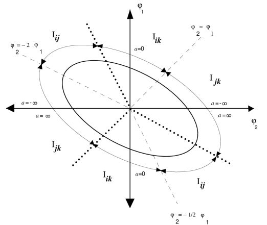
Figure 3:

Figure 4:

Figure 5a :

Figure 5b :