STRING FINE TUNING

G.Savvidy, K.Savvidy

Institut für Theoretische Physik der Universität Frankfurt,

D-6000 Frankfurt am Main 11,Fed.Rep.Germany

..hat man die eine,
die synthetische (Methode),
sehr vernachlässigt…
Jacob Steiner.

Abstract

We develop further a new geometrical model of a discretized string, proposed in [1] and establish its basic physical properties. The model can be considered as the natural extension of the usual Feynman amplitude of the random walks to random surfaces. Both amplitudes coinside in the case , when the surface degenerates into a single particle world line. We extend the model to open surfaces as well. The boundary contribution is proportional to the full length of the boundary and the coefficient of proportionality can be treated as a hopping parameter of the quarks. In the limit, when this parameter tends to infinity, the theory is essentially simplified. We prove that the contribution of a given triangulation to the partition function is finite and have found the explicit form for the upper bound. The question of the convergence of the full partition function remains open. In this model the string tension may vanish at the critical point, if the last one exists, and possess a nontrivial scaling limit. The model contains hidden fermionic variables and can be considered as an independent model of hadrons.

1 Introduction.

It is well known, that lattice regularisation of gauge theories can be used to define the theory non-perturbatively [3]. In analogy with this it is important to find non-perturbative regularisation of the string in order to understand its complicated dynamical properties. At the same time interacting random surfaces should play an important role in describing quantum fluctuations of the gauge systems at least in confining phase [3]. The purpose of this paper is to develop and to study a geometrical model of discretized string, which has been recently proposed in [1].

Definition of the random surfaces model by dynamical triangulation (DT) allows to investigate many interesting models [2-6]. In this approach continuum random surfaces are represented by triangulated surfaces. Then in order to describe statistical properties of two-dimensional surfaces, randomly immersed into d-dimensional space $R^{d}$, it remains to choose a suitable classical action. If the action is defined as the sum of the areas of the individual triangles, making up the surface- $A(S)$, then the partition function is ill defined, because the area action does not suppress ”spiky” configurations [2,15]. If the action is proportional to the length of all edges in a triangulation T, that is the gaussian model with the action $A(L)$, then the string tension does not scale at the critical point and the continuum limit is also questionable [7]. Therefore it is not clear, whether there is one or many universal classes of random surfaces, which are relevant for the solution of the problems, mentioned above.

One of the possible conclusions, which can be done from these results, consists in the fact, that in order to reach a non-trivial continuum limit the classical action of the DT random surfaces must be chosen in the way to fulfil appropriate scaling behaviour. We shall call this dynamical adjustment of the classical action to convenient scaling behaviour of the model as string fine tuning.

The question, which arises here, can be formulated in the following way: is there any simple principle, which allows to make a natural choice of the classical action for DT surfaces, prior to solving the model?

A new guiding principle was suggested in [1]. This geometrical principle demands, that two surfaces, distinguished by a small deformation of the shape in the embedding space, must have close actions, that is, these surfaces must have the same statistical weight.

This principle is very restrictive and allows only few possibilities. Let us for example consider area action $A(S)$ and gaussian action $A(L)$. In both cases the action is continuous with respect to a small deformation of the DT surface, when we change the coordinates of the vertexes of a given triangulation $T$. However, the continuity of the action $A$ in the space of all triangulations $\{T\}$ requires careful examination. Indeed, let us consider two triangulations $T_{1}$ and $T_{2}$ with different numbers of vertexes, $N_{1}$ and $N_{2}$, but with the same Euler characteristic. There always exists such a position of these vertexes, that these two surfaces geometrically coincide. Therefore the difference $\delta A=A^{T_{1}}-A^{T_{2}}$ must tend to zero in accordance with our principle and this must hold good independently of the number of vertexes. It is easy to check, that the area action $A(S)$ possesses the defined property, but the functional $A(L)$ does not [1]. Therefore the probability distribution in the space of all triangulations $\{T\}$ is continuous for the action $A(S)$ and is discontinuous for the action $A(L)$.

The question is, whether there are any new functionals with the same properties, that is, they are positive and continuous in the space of all triangulations $\{T\}$ and invariant under euclidean group of transformations. The answer is yes [1]. Steiner functional [11] had these desirable properties, except for the positivity. But it can be extended in a such a way, that it will fulfil positivity condition as well [1] (see below).

As a result we have an action, which is modified Steiner functional [1]

$$A(M)=1/2\sum_{<i,j>}|X_{i}-X_{j}|\cdot\Theta(\alpha_{i,j}),$$

where

$$\Theta(\alpha)=|\pi-\alpha|$$

and summation is over all edges $<X_{i},X_{j}>$ in triangulation T and $\alpha_{i,j}$ is the angle between the embedded neighbour triangles in $R^{d}$, having a common edge $<X_{i},X_{j}>$ (see Fig.1). This action indeed has desirable properties.

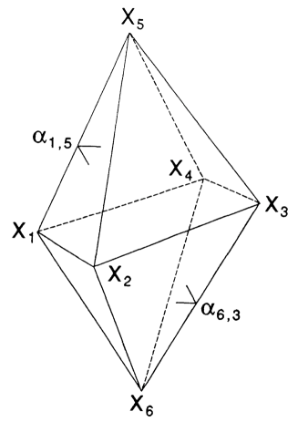
Figure 1: The $A(M)$ is equal to $A(M)=1/2\sum_{<i,j>}|X_{i}-X_{j}|\cdot|\pi-\alpha_{i,j}|$

.

Thus DT surfaces, weighted by the area action $A(S)$ or by this action $A(M)$, have continuous distribution of the statistical weights in the space of all triangulations $\{T\}$. From other side, a partition function of the DT surfaces is ill defined for the area action $A(S)$ and converges for the gaussian action $A(L)$. The first question, which arises here, is connected with the existence of the partition function for the theory with the action $A(M)$. In this article we will prove, that the contribution $Z_{T}$ of a given triangulation $T$ to the partition function $Z$ is finite. The upper bound, which we find out for these terms, does not permit us to state, that the full partition function exists, but we expect, that it is possible to improve this bound, because it is not the best. Therefore this geometrical model still can be considered as possible variety of discretised string.

At the beginning we shall present simple qualitative arguments, demonstrating the convergence of the partition function $Z$ [1]. The partition function of our surface model is

$$Z(\beta)=\sum_{oversurfaces}e^{-\beta\cdot A(M)}=\sum_{T\in\{T\}}Z_{T}(\beta).$$

The first argument is based on Minkowski inequality [10] (see also [9,12]), which tells, that on arbitrary surface the functional $A(M)$ is always greater, than the square root of the surface area

$$A^{2}(M)\geq 4\pi S,$$

and equality takes place only for sphere, that is, among all surfaces with fixed area, the sphere has minimal $A(M)$. From (3) one can conclude, that the convergence of the partition function is in any case better than for the area action, because

$$e^{-A}\leq e^{-\sqrt{4\pi S}},$$

and that the maximal distribution carries the surfaces, close to sphere. This fact has very elegant consequence: quasi-classical expansion, when $\beta\rightarrow\infty$, must be done around sphere. In that regime there is no big difference between area action and $A(M)$ action. This is especially valuable, because strong coupling expansion of the gauge theory on a lattice is described by the area action [3].

As we already explained, the action (1) is not exactly the Steiner functional, and inequality (3) was established only for convex surfaces. Initially the Steiner functional was written for convex surfaces and for them $\Theta$ is equal to $\pi-\alpha$ [11]. For our purposes we need a certain extension of the classical Steiner functional to all surfaces. The extension (1) is made up in a such a way, that the action is always positive and concave surfaces with the same area have larger action than the convex ones. Therefore, for the modified functional $A(M)$ inequality (3) takes place for all surfaces. The inequality (3) is very important for the physical interpretation of $A(M)$, because it establishes an absolute minimum of the functional $A(M)$ and guarantees, that the surfaces will not collapse with large probability to crumple surfaces. Note, that this extension also provides $\it locality$ of the classical action [1].

The next qualitative argument, displaying the convergence of the partition function, consists in the observation, that the Steiner functional for the convex surfaces geometrically is the $\it mean$ $\it size$ of the surface [12-14]

$$A(M)=\int L_{g}\ dg,$$

where $L_{g}$ is the length of the orthogonal projection of the surface T to the line $g$, which crosses the origin in $R^{d}$. $dg$ is the invariant measure of these lines [14-16] . For example, if $T$ is sphere, then $L_{g}=2R$ and $A(M)=4\pi R$ . It is easy to see from (4), that $A(M)$ increases with the diameter $\Delta$ of the surface (here $\Delta$ is the largest distance between two points on the surface), so the statistical weight of the surface decreases. For example, spiky configurations are strongly suppressed, because they have large size. In the case of area action, the action does not always increase with the diameter of the surface and the corresponding weights can even be constant.

In the next section we rigorously define the surface action $A(M)$ (1) [1]. We present the necessary geometrical properties of this functional and consider few examples. In fact, if the surface degenerates into single curve, the action $A(M)$ becomes proportional to a full length of the curve and transition amplitude coincides with the one for the Feynman path integral. This means that $A(M)$ is the natural extension of usual Feynman amplitude of the random walks to random surfaces.

If the surface has boundaries, ”created by virtual quarks or by external sources”, then the boundary part of the action is proportional to the full length of the boundary. The coefficient of proportionality can in principle be changed (see (2b)) and treated as the hopping-parameter of the quarks. The limit, in which this parameter tends to infinity, corresponds to pure QCD, otherwise we would have dynamical quarks. Here we use QCD terminology merely because random surfaces should describe the fluctuation of gauge degrees of freedom at least in confining phase, but certainly these results do not depend on the use of this analogy. In same sense one can consider this model as an independent theory.

In the third section we prove that the contribution $Z_{T}$ of a given triangulation $T$ to the partition function $Z$ is finite. At the begining we will find the following bound

$$Z_{T}\leq(Const\cdot 2^{|T|/2})^{d(|T|-1)}$$

where $|T|$ is the number of vertexes and $d$ is the dimention of the space. Then, using ”shape” coordinates [15], we improve this bound and find, that

$$Z_{T}\leq(Const)^{d(|T|-1)}\cdot(d(|T|-1))!$$

This bound does not permit to prove the convergence of the full partition function, but it is important to note, that the volume of the ”shape” coordinates was crudely estimated. Therefore we expect that it is possible to improve this bound. This section is more technical, but permits to clarify contents of the theory, particularly geometrical meaning of the extension (1).

The fourth section is devoted to the discussion of the critical behaviour of the model and we will show that the theorem of Ambjorn and Durhuus [7], concerning the non-vanishing of the string tension of the gaussian model, is not valid in our case, so the string tension may tend to zero at the critical point. In the last section we discuss possible extensions of this model and compare them with the gaussian one.

2 Geometrical and physical properties of $A(M)$

Let us consider closed surfaces in $R^{d}$, given by the mapping of the vertices of some fixed triangulation T into the euclidean space $R^{d}$ [2]. Triangulations T are defined as connected, two-dimensional abstract simplical complexes with fixed topology [2]. The surfaces to be identified with a piecewise linear surfaces embedded into $R^{d}$ (see fig.1). The coordinates of the vertexes in $R^{d}$ are denoted as $X_{i}^{\mu}$, where $\mu=1,..,d$ and $i=1,..,|T|$ . $|T|$ is the number of vertexes on T. We shall use the same letter T to denote the surface. The action is given by [1]

$$A(M)=1/2\sum_{<i,j>}|X_{i}-X_{j}|\cdot\Theta(\alpha_{i,j}),$$

where

$$\Theta(\alpha)=|\pi-\alpha|$$

and summation is over all edges $<X_{i},X_{j}>$ ( i and j are the nearest neighbours in T ), $\alpha_{i,j}$ is the angle between the embedded neighbour triangles in $R^{d}$ having a common edge $<X_{i},X_{j}>$. This expression essentially differs from the gaussian action $A(L)$, because here all lengths of the edges are directly multiplied by the corresponding angles $\Theta(\alpha_{i,j})$ (see fig.1). This means that the edges are weighted in a more complicated way compared to a gaussian model: sometimes they contribute in full,$\alpha\approx 0,2\pi$, sometimes they do not contribute at all, $\alpha\approx\pi$. This circumstance provides the action $A(M)$ by peculiar geometrical and physical properties.

As it was already explained, the module in (2) corresponds to a specific extension of the Steiner functional to all surfaces. The extension (1) coincides with the Steiner functional for convex surfaces and therefore inherits the same geometrical nature. At the same time, extension (1) provides relative suppression of the crumple surfaces, because for them $\alpha$ is close to zero or to $2\pi$, so $\Theta$ is in its maximum. Finally we have locality of the classical action.

To have some intuitive experience let us consider few examples. The action $A(M)$ has the dimension of the length and expresses, as it follows from the definition (1) and representation (4), the mean size of the surface. Therefore even when the surface degenerates into a thin tube, the action does not vanish, as it happens in the case of area action, because this tube has non zero size. If the surface degenerates into a single curve, then it is easy to see from the definition (1), that the action is proportional to the full length $L$ of that curve

$$A(M)=L/2\cdot\pi.$$

So $A(M)$ correctly weights degenerated surfaces, it is proportional to the full length of the curve, and the transition function coincides with the one for the Feynman path integral.This means that $A(M)$ is the natural extention of usual Feynman amplitude of the random walks to random surfaces. The area action is unable to describe such surfaces and the gaussian action ”over-count” these configurations.This leads to spikes, growing out of the surface in the model with area action, and to non-scaling behaviour of the string tension in the gaussian model [2,7].

The coefficient of proportionality on the right-hand side of (5a) coded the information about the way the surface squeezed into the curve. For example, if the surface collapsed and crumpled, then this coefficient increases and is equal to the number of crinkles

$$A(M)=L/2\cdot k\pi,$$

where $k$ is the number of crinkles.

Up to now we have considered only closed surfaces, but the definition (1) has natural meaning for the open surfaces as well. It is reasonable to take $\alpha_{i,j}$ on the boundary edges equal to zero or to $2\pi$. Then from the definition (1) it follows, that the boundary part of the action is proportional to the full length of the boundary

$$A(M)_{boundarycontribution}=L/2\cdot\pi,$$

where $L$ is the full length of the boundary. This fact has important physical consequence: the quark loop amplitude is proportional to the length of their world line. Let us consider an extension of the action (1), in which $\Theta$ satisfies to more general conditions [1]

$$\Theta(2\pi-\alpha)=\Theta(\alpha),$$

$$\Theta(\pi)=0,$$

$$\Theta(\alpha)\geq 0,$$

then we will get

$$A(M)_{boundarycontribution}=L/2\cdot\Theta(0).$$

So the full length of the boundary is multiplied by $\Theta(0)$. $\Theta(0)$ plays the role of the hopping-parameter of the quarks. In fact, if we take $\Theta(0)$ to be very large, then the probability of the quark loop creation tends to zero (see (6b) and one can treat $\Theta(0)$ as the logarythm of the quark masses. At the same time, in the limit $\Theta(0)\rightarrow\infty$ the string tension may have finite limit, because, as we will see in the next section, string tention is formed by fluctuations of the surface near $\alpha\approx\pi,\Theta(\pi)\approx 0$. These fluctuations do not disappear even if $\Theta(0)=\infty$ (see (2b). If so, then this limit corresponds to pure $QCD$, that is, quarks are not dynamical. When $\Theta(0)\rightarrow\pi$, then we will have dynamical quarks.

At the end of this section we would like to emphasise, that unless the action $A(M)$ has many different representations, we consider the expression (1) as more fundamental, because it is well defined for extremely large class of surfaces, including degenerate surfaces. The model is well defined in any dimension and for arbitrary topologies. Of course it coincides with other expressions in special cases.

It is also important to note, that this model can be considered as a sort of a theory with extrinsic curvature action [19,20,1].

3 The partition function

Partition function is defined usually as in [2]

$$Z(\beta)=\sum_{T\in\{T\}}\rho(T)\int e^{-\beta A(M)}\prod_{i\in T}dX_{i},$$

where $\{T\}$ denotes some set of closed triangulations T , $\rho(T)$ are their weights, $dX_{i}$ are the measures in $R^{d}$. One vertex $X_{f}^{\star}$ is fixed to remove translation invariant zero-mode and we should specify the summation weight $\rho(T)$ in the definition (7).This can be done as a consequence of our first geometrical principle. It demands, that the distribution of the statistical weights must be continuous in the space of all triangulations $\{T\}$.To satisfy this condition we must choose $\rho(T)=1$ .

Now we would like to prove, that the contribution of a given triangulation $T$ to the partition function is finite and would like to find the explicit form of the upper bound. With this aim, in our first approach we will successively perform the integration over all vertexes in T.

For a while let us denote the coordinates of the arbitrarily chosen vertex $X_{i}$ by $X$ and its nearest neighbour vertexes by $X_{1},..,X_{q}$. They are ordered cyclically around $X$ and $q$ is the order of $X$ (the number of ingoing edges). The vertex of the triangle, which lies opposite to the triangle $<X,X_{i},X_{i+1}>$ and has a common edge $<X_{i},X_{i+1}>$, we will denote by $Y_{j}$, where $j=1,..,p$ and $1\leq p\leq q$ (see fig.2).

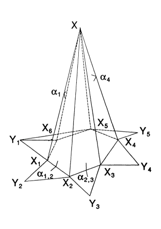
Figure 2: The $A(M)$ depends on $X$ through the length of the edges $|X-X_{i}|$ and through the compact angle variables $\alpha_{i}$ and $\alpha_{i,i+1}$ .

The part of the classical action $A(M)$ (1), which depends on $X$, has the form:

$$A(M)=A_{x}+A_{xy}+A,$$

$$A_{x}=\sum_{i=1}^{q}|X-X_{i}|\cdot\Theta(\alpha_{i}),$$

$$A_{xy}=\sum_{i=1}^{q}|X_{i}-X_{i+1}|\cdot\Theta(\alpha_{i,i+1}),$$

where

$$\Theta(\alpha_{i})=|\pi-\alpha_{i}|,$$

$$\Theta(\alpha_{i,i+1})=|\pi-\alpha_{i,i+1}|$$

and $X_{q+1}=X_{1}$. The $\alpha_{i}$ is the angle between two triangles, having common edge $<X,X_{i}>$ and $\alpha_{i,i+1}$ is the one with a common edge $<X_{i},X_{i+1}>$ (see Fig.2). This decomposition is very natural, because $A_{x}$ depends on $X$ through the length of the edges $|X-X_{i}|$ and through the corresponding compact angle variables $\alpha_{i}$. As far as $A_{xy}$ is concerned, it depends on $X$ only through the compact variables $\alpha_{i,i+1}$. The integral over $X$ has the form

$$Z(X_{i},Y_{j})=\int e^{-A_{x}-A_{xy}}dX,$$

where

$$e^{-A_{x}}\equiv g(X,X_{i}),$$

$$e^{-A_{xy}}\equiv f(X,X_{i},Y_{j}).$$

It seems reasonable to use the bound $e^{-A{xy}}\leq 1$ in (13) and then to prove the convergence of the remaining integral (see (16). But in that case the next integration over the nearest neighbour vertex $X_{i}$ will create difficulties, because $A_{xy}$ has few terms of the action with edge angles $\alpha_{i,i+1}$, which also belong to a vertex $X_{i}$ . These terms will be absolutely nessesary, when we will perform integration over $X_{i}$, because they allow to bind the sum of all edge angles, belonging to $X_{i}$, from below (see (19),(20)). So, we will treat the term $e^{-A_{xy}}$ in a more gentle way, that is we would like to find following expression for $Z$ after integration over $X$ in (13),

$$Z(X_{i},Y_{j})=Const\cdot e^{-A_{x^{*}y}},$$

where $X^{*}$ is an ”average” position of the vertex $X$. Following inequality takes place:

$$m\cdot e^{-A_{x}}\leq e^{-A{x}-A_{xy}}\leq M\cdot e^{-A_{x}},$$

in which $M(X_{i},Y_{j})$ and $m(X_{i},Y_{j})$ are the maximum and minimum of the function $f(X,X_{i},Y_{j})$ over $X$ at fixed $X_{i}$ and $Y_{j}$. The function $f(X,X_{i},Y_{j})$ continuously depends on $X$ through the compact angle variables $\alpha_{i,i+1}$, therefore the maximum and minimum actually exist (Weierstrass theorem). Now let us prove the convergence of the integral

$$Z(X_{i})=\int e^{-A_{x}}dX.$$

Let denote by $r$ the minimal radius of the sphere, which contains all vertexes $X_{1},..,X_{q}$ and choose the origin in the centre of that sphere. Then we will have

$$Z(X_{i})=\int_{|X|\leq 2r}e^{-A_{x}}dX+\int_{|X|\geq 2r}e^{-A_{x}}dX.$$

Inside sphere, in the first integral, one can bound the integrant by one

$$\int_{|X|\leq 2r}e^{-A_{x}}dX\leq{\pi^{d/2}\over\Gamma(1+d/2)}\cdot(2r)^{d}$$

and change every edge length $|X-X_{i}|$ by smaller quantity $|X|-r$ in the second integral

$$\int_{|X|\geq 2r}e^{-A_{x}}dX\leq\int_{|X|\geq 2r}e^{-(|X|-r)\sum_{i=1}^{q}\Theta(\alpha_{i})}dX.$$

We must bound the sum of all edge angles, belonging to vertex $X$, from below. The desirable answer is

$$0<\Theta_{min}\leq\sum_{i=1}^{q}\Theta(\alpha_{i})\leq q\pi.$$

The proof of this fact will be presented in separate place. It is important to note, that this number $\Theta_{min}$ does not depend on $r$ and $q$, but depends on proportion $k$, by which the integral (16) was divided into two parts (see (17)).For $d=3$ we get

$$\Theta_{min}=2\pi\cdot\sqrt{(1-k^{-2})},$$

and if $k=2$, as it was in (17),

$$\Theta_{min}=\pi\sqrt{3}.$$

Inserting (20a) in (19) we get

$$\int_{|X|\geq 2r}e^{-(|X|-r)\cdot\Theta_{min}}dX=$$

$${2\pi^{d/2}\over\Gamma(d/2)}\cdot e^{\Theta_{min}r}\cdot\int_{2r}^{\infty}e^{-|X|\Theta_{min}}(|X|)^{d-1}\,dX\leq\left(Const\over\Theta_{min}\right)^{d}.$$

The radius $r$ is always smaller than the sum of all distances between $X_{1},..,X_{q}$

$$r\leq\sum_{i=1}^{q}|X_{i}-X_{i+1}|,$$

thus

$$Z(X_{i})\leq\left[Const\sum_{i=1}^{q}|X_{i}-X_{i+1}|\right]^{d}$$

It is helpful to compare this bound with the same quantity for the model with area action [2]

$$Z(X_{i})=\int e^{-A_{x}(S)}dX\geq 1/{\left[Const\sum_{i=1}^{q}(X_{i}-X_{i+1})^{2}\right]^{d/2}}.$$

The difference consists in the fact, that in our case the weight function is equal to one in the region of order $r$, while for the model with area action the same region is of order $1/r$.

Because the last integral (23),(16) is finite, one can integrate inequality (15) over $X$

$$m\cdot Z(X_{i})\leq Z(X_{i},Y_{j})\leq M\cdot Z(X_{i}),$$

or

$$m\leq{Z(X_{i},Y_{j})\over Z(X_{i})}\leq M.$$

This relation is a direct analog of the classical formula from calculus

$$m\leq{\int_{-\infty}^{\infty}f(X)g(X)dX\over\int_{-\infty}^{\infty}g(X)dX}\leq M,$$

where $g(X)$ is an integrable function in $[-\infty,\infty]$ and $m\leq f(X)\leq M$, so

$$\int_{-\infty}^{\infty}f(X)g(X)dX=f(X^{\star})\int_{-\infty}^{\infty}g(X)dX.$$

The $f(X,X_{i},Y_{j})$ is continuous function of $X$ and takes all its values between $m(X_{i},Y_{j})$ and $M(X_{i},Y_{j})$ (Bolzano-Cauchy theorem), therefore there exists such a position of the vertex $X=X^{\star}$, for which

$$Z(X_{i},Y_{j})=f(X^{\star},X_{i},Y_{j})\cdot Z(X_{i}),$$

or

$$Z(X_{i},Y_{j})=e^{-\sum_{i=1}^{q}|X_{i}-X_{i+1}|\cdot\Theta(\alpha_{i,i+1}^{\star})}\cdot Z(X_{i}).$$

Using (23) we get

$$Z(X_{i},Y_{j})\leq e^{-\sum_{i=1}^{q}|X_{i}-X_{i+1}|\cdot\Theta(\alpha_{i,i+1}^{\star})}\cdot\left[Const\sum_{i=1}^{q}|X_{i}-X_{i+1}|\right]^{d},$$

where

$$\alpha_{i,i+1}^{\star}=\alpha_{i,i+1}(<X^{\star},X_{i},X_{i+1}>,<X_{i},X_{i+1},Y_{i}>)$$

So the quantity $Z(X_{i},Y_{j})$ is finite and we preserve the part of the action, which contains the edge angles $\alpha_{i,i+1}$. Now they can ”participate” in the subsequent integration over all $X_{i}$ and permit to bound the sum of all edge angles, belonging to $X_{i}$, from below, as it was already done for the vertex $X$ (19-21).

The main trouble consists in the fact, that the vertex $X^{\star}$ can in principle be settled down on infinity, because in that point $f(X,X_{i},Y_{j})=e^{-A_{xy}}$ is non zero and finite. The last circumstance insists on us to change slightly the strategy. We shall use another decomposition in (13)

$$Z(X_{i},Y_{j})=\int h^{2}dX,$$

where

$$h=e^{-(A_{x}+A_{xy})/2}.$$

Repeating calculations for the last decomposition, we will get

$$Z(X_{i},Y_{j})=h^{\star}\cdot\int hdX\leq Const\cdot h^{\star},$$

where

$$h^{\star}=e^{-(A_{x^{\star}}+A_{x^{\star}y})/2}=e^{-1/2\sum_{i=1}^{q}|X^{\star}-X_{i}|\cdot\Theta(\alpha_{i}^{\star})+|X_{i}-X_{i+1}|\cdot\Theta(\alpha_{i,i+1}^{\star})}$$

and

$$\alpha_{i}^{\star}=\alpha_{i}(<X^{\star},X_{i},X_{i-1}>,<X^{\star},X_{i},Y_{i+1}>).$$

Now the vertex $X^{\star}$ is sited on a finite distance from the vertexes $X_{i}$ and $Y_{j}$. In fact, the function $h(X,X_{i},Y_{j})=e^{(-A_{x}-A_{xy})/2}$ reaches the minimum at infinity, because at that point $|X^{\star}|=\infty$, the value of the $A_{x^{\star}}=\infty$ and thus $h^{\star}=0$. But the value of full integral (32) is strictly positive, therefore the ”average” vertex $X^{\star}$ cannot be at infinity (see (33)).

The final result of the integration over the vertex $X$ consists in three facts:

i)now two of the initial vertexes are fixed $X_{f}^{\star}$ and $X^{\star}$, but the position of the average vertex $X^{\star}$ depends on its neighbour vertexes $X_{i}$ and $Y_{j}$ ,

ii)the effective classical action does not change its own geometrical nature,that is all terms, belonging to the vertex $X^{\star}$, still remain (33),

iii)the effective action decreases by the factor two (33).

From (32) we get

$$\int e^{-A(M)}\prod_{i\in T\setminus X_{f}^{\star}}dX_{i}=$$

$$\int e^{-(A_{x^{\star}}+A_{x^{\star}y})/2}\cdot e^{-A-(A_{x}+A_{xy})/2}\cdot\prod_{i\in T\setminus X_{f}^{\star}}dX_{i}\leq$$

$$Const\cdot\int e^{-(A_{x^{\star}}+A_{x^{\star}y})/2}\cdot e^{-A}\prod_{i\in T\setminus X_{f}^{\star},X^{\star}}dX_{i}\leq$$

$$Const\cdot\int e^{-(A+A_{x^{\star}}+A_{x^{\star}y})/2}\prod_{i\in T\setminus X_{f}^{\star},X^{\star}}dX_{i},$$

Now it remains to integrate over the rest vertexes. Below we will assume, that the vertex $X^{\star}$ depends on $X_{i}$ and $Y_{j}$ in a such way, that it is always sited within the region of the sphere of radius $r$ (22), which contains all vertexes $X_{1},..,X_{q}$. Then every subsequent integration will change the exponent by the factor $1/2$, so finally we get

$$Z_{T}\leq(Const\cdot 2^{|T|/2})^{d(|T|-1)}\cdot e^{-A(M^{\star})/{2^{|T|-1}}},$$

where all vertexes in $A(M^{\star})$ are ”imaginary” and are situated on a finite distance from each other. The constant on the right-hand side of (36) depends only on d .

From (36) and (7) it follows, that

$$Z(\beta)\leq\sum_{T\in\{T\}}(Const\cdot 2^{|T|/2}/\beta)^{d(|T|-1)},$$

but this bound is not sufficient to prove the convergence of the full partition function. It is useful to compare this bound with the one in the gaussian model [19].

Let us return to our assumption of the ”week” dependence of the vervex $X^{\star}$ from its neighbours. To control this dependence we must take into account the fact that the full action $A(M)$ is the mean size of the surface and therefore $X^{\star}$ can not ”run” far away from the origin (which we will take in the fixed point $X_{f}^{\star}$). Explicit estimates are very fragile, because we must use a local and global properties of $A(M)$ at the same time.

In this place we came to a point, that the convergence can be proved only by using global character of $A(M)$. Indeed

$$A(M)\geq\Delta,$$

where $\Delta$ is the diameter of the surface (largest distance between two points on the surface) and let us define $R$

$$R=\sqrt{X^{2}_{1}+....+X^{2}_{|T|-1}}\leq\sqrt{(|T|-1)}\cdot\Delta,$$

where the origin is in the point $X_{f}^{\star}$. So we have

$$A(M)\geq R/\sqrt{(|T|-1)}$$

and therefore for $Z_{T}$ we will get

$$\int e^{-A(M)}\prod_{i\in T\setminus X_{f}^{\star}}dX_{i}\leq$$

$${2\pi^{d(|T|-1)/2}\over\Gamma(d(|T|-1)/2)}\cdot\int_{0}^{\infty}e^{-R/\sqrt{|T|-1}}R^{d(|T|-1)-1}\,dR=$$

$${2\pi^{d(|T|-1)/2}\over\Gamma(d(|T|-1)/2)}\cdot(|T|-1)^{d(|T|-1)/2}\cdot{(d(|T|-1))!\over d(|T|-1)}$$

The third possibility is to introduce a new coordinate system in which $A(M)$ is an independent variable. A remaning part of the variables we will take as angles $\vec{\alpha}$ or ”shape” variables [15] (they don’t coincide with $\alpha_{i,j}$) , so we have

$$\int\prod_{i\in T\setminus X_{f}^{\star}}dX_{i}=\int A(M)^{d(|T|-1)-1}\cdot J(\vec{\alpha})\,dM(A)\,d\vec{\alpha},$$

where $J(\vec{\alpha})$ is the Jacobean of this transformation. Integrating both sides over the $X^{\prime}s$ in $R^{d}$ with the condition, that for them $A(M)\leq A$, we will get

$$\int J(\vec{\alpha})\,d\vec{\alpha}=\int_{\leq A}\prod_{i\in T\setminus X_{f}^{\star}}\,dX_{i}/\int_{0}^{A}A(M)^{d(|T|-1)-1}\,dM(A).$$

Because every coordinates $X^{\prime}s$ are bounded at list in the region $0\leq|X_{i}|\leq A$, it follows, that

$$\int J(\vec{\alpha})\,d\vec{\alpha}\leq d(|T|-1)\cdot\left({\pi^{d/2}\over\Gamma(1+d/2)}\right)^{|T|-1}.$$

Therefore for full integral we will get

$$\int e^{-A(M)}\prod_{i\in T\setminus X_{f}^{\star}}dX_{i}=$$

$$\int e^{-A(M)}A(M)^{d(|T|-1)-1}\cdot J(\vec{\alpha})\,dM(A)\,d\vec{\alpha}\leq(d(|T|-1))!\left({\pi^{d/2}\over\Gamma(1+d/2)}\right)^{|T|-1}$$

By the same technic one can prove, that the contribution of a fixed triangulation to the loop Green functions are also finite, but this bound still leave the question of the full convergence open.

4 Loop Green functions

The loop Green functions can be defined as usually [2]:

$$G_{\beta}(\gamma_{1}...,\gamma_{n})=\sum_{T\in\{T\}}\rho(T)\int e^{-\beta A(M)}\prod_{i\in T\setminus\partial T}dX_{i}$$

where $\gamma_{1}...,\gamma_{n}$ are closed polygonal loops in $R^{d}$ with $k_{1}..,k_{n}$ corners, and $\{T\}$ denotes the set of triangulations with $n$ boundary components.

If the loop Green functions are finite for sufficiently large $\beta$, then one can define string tension [2]

$$\sigma(\beta)=-\lim_{R,L\rightarrow\infty}\ln G_{\beta}(\gamma_{R,L})/{RL},$$

where $\gamma_{R,L}$ is rectangle with sides of length $R$ and $L$. Ambjorn and Durhuus have proved, that string tension of the gaussian model does not vanish at the critical point, because the minimal surface dominates in the functional integral.Quantum fluctuation does not contribute and cannot lower the ”classical” string tension [7]. They found, that [7]

$$G_{\beta}(\gamma_{R,L})\leq e^{-2\beta RL}\cdot G_{\beta}(O_{R,L}).$$

The $G_{\beta}(O_{R,L})$ is the loop Green function, where the loop $\gamma_{R,T}$ is contracted into one point $O$. For this Green function they found the bound [7]

$$G_{\beta}(O_{R,L})\leq e^{C(\beta)\cdot(R+L)},$$

where $C(\beta)$ is finite for $\beta>\beta_{c}>0$, thus [7]

$$\sigma(\beta)\geq 2\beta.$$

and string tension does not vanish at $\beta_{c}$.

In our case we have, that

$$A(M_{R,L})=A_{min}(M_{R,L})+A(M,O_{R,L}),$$

where $A_{min}(M_{R,T})$ is the minimum of $A$ for the surfaces with rectangular boundary $\gamma_{R,L}$ and $A(M,O_{R,L})$ is the remaining part of the action. It is easy to see, that

$$A_{min}(M_{R,L})=2(R+L)\cdot\pi.$$

Inserting (42-43) in (37), we get

$$G_{\beta}(\gamma_{R,L})=e^{-\beta(R+L)\cdot\pi}\cdot G_{\beta}(O_{R,L}),$$

so the minimal surface does not contribute at all (compare with (39)). Only quantum fluctuations are important:

$$\sigma(\beta)=-\lim_{R,L\rightarrow\infty}\ln G_{\beta}(O_{R,L})/{RL}.$$

For the general model (2b) we will get

$$G_{\beta}(\gamma_{R,L})=e^{-\beta(R+L)\cdot\Theta(0)}\cdot G_{\beta}(O_{R,L}).$$

Let us consider the case, when $\Theta(0)\to\infty$. In this limit the theory is essentialy simplified. In fact, all fluctuations, in which the surface considerably crumpled, that is $\alpha$ is close to zero or to $2\pi$ and $e^{-A(M)}\to 0$, are strongly suppressed. Nevertheless, in this limit the surface with the boundary $\gamma_{R,L}$ can fluctuate near the angles $\alpha\approx\pi$, where $\Theta(\alpha)$ is close to zero. Now one can estimate contribution of such fluctuations to the loop Green function

$$G_{\beta}^{T}(\gamma_{R,L})\approx a^{T}\cdot e^{-\sigma_{T}(\beta)\cdot RL}.$$

The difference with the gaussian model consists in slower decrease of the series expansion (37). To convince of that let us use the inequality

$$A(M)\leq(\sum_{<i,j>}|X_{i}-X_{j}|)\cdot(\sum_{<i,j>}\Theta(\alpha_{i,j}))\leq\sum_{<i,j>}|X_{i}-X_{j}|\cdot 3\pi(|T|-Euler\cdot charac.),$$

so for torus

$$e^{-3\pi|T|\cdot A^{T}(L)}\leq e^{-A^{T}(M)}$$

Therefore the string tension may have nontrivial scaling limit in this theory.

5 Discussion

It is useful to compare (1) with the gaussian model. For that let us consider the action

$$A=\sum_{<i,j>}(X_{i}-X_{j})^{2}(1+g\cos(\alpha_{i,j})),$$

where $g$ is the coupling constant $0\leq g\leq 1$. If $g=0$, then this model coincides with gaussian one and, if $g=1$, it coinsides with (1), (2b), where

$$\Theta(\alpha)=1+\cos(\alpha),$$

just in (46) we have the squares of the lengths.

When $g\neq 1$, the edges contribute with the weights, variating in the region $[(1-g)(X_{i}-X_{j})^{2};(1+g)(X_{i}-X_{j})^{2}]$. These weights do not vanish for all values of the angle $\alpha_{i,j}$,

$$e^{-(1+g)\sum_{<i,j>}(X_{i}-X_{j})^{2}}\leq e^{-A}\leq e^{-(1-g)\sum_{<i,j>}(X_{i}-X_{j})^{2}}$$

The critical temperatures for these boundary models are equal to $\beta_{c}/(1+g)$ and $\beta_{c}/(1-g)$ respectively.The critical exponents are the same ones.

For the most interesting point $g=1$ the weight function can vanish, $\Theta(\pi)=0$ (see (47),(46)), and does not permit us to find the bound. Exactly the same property ensures the continuity of the $A(M)$ in the space of all triangulations [1], that is why the model was examined separatelly.

The model, in which boundary contribution can variate (see (6b)) , has the form

$$A=\sum_{<i,j>}(X_{i}-X_{j})^{2}(1+\cos(\alpha_{i,j}))/{(1-g\cos(\alpha_{i,j}))},$$

where

$$\Theta(\alpha)=1+\cos(\alpha)/{1-g\cos(\alpha)}.$$

The quark loop amplitude is proportional to

$$e^{-\beta\cdot\Theta(0)\cdot L},$$

where

$$\Theta(0)=2/(1-g).$$

Pure $QCD$ corresponds to $g=1$. The last two models can help to perform analytical calculations and Monte-Carlo simulations. They are probably in the same universal class.

In the forthcoming publication we shall present more details concerning the inequality (3), which plays crucial role in this theory and establishes an absolute minimum of the Steiner functional $A(M)$. On the plane it reduces to the well known isoperimetric inequality [8]. The isoperimetric inequality has very long history [8-10] and in the case of a curve on the plane it states, that $L^{2}\geq 4\pi S$, where $L$ is the perimeter of the curve and $S$ is the enclosed area, equality takes place only for circle. As it already was mentioned,the inequality (3) is also reduced to equality only for the sphere. In this theory the sphere plays the role of instanton [1,17,18]. The decomposition (42) has also deep geometrical origin and is connected with linear property of $A(M)$.

Finally let us project $A(M)$ onto one- and two-dimensional spaces. In $R^{2}$ the image of the squeezed surface is reduced to a polygon with the vertexes $X_{1},..,X_{|T|}$. The action $A(M)$ becomes proportional to the length of the ”shadow” polygon sides, but the difference with the gaussian model is that in this case only sides, attached to round curves, are distributed (the surface squeezed without crinkles). In principle one can consider this picture as the new version of the gaussian model in $2d$. In $R^{1}$ $A(M)$ is reduced to the diameter $r$ of the vertexes.

We gratefully acknowledge conversations with R.Ambartzumian, I.Batalin,E.Floratos, G.Flume, A.Kaidalov, B.Müller, H.Nielsen and G.Sukiasian.

One of the authors (G.S.) is thankful to R.Ambartzumian, who twenty years ago introduced him into the beautiful Buffon’s problem of the needle and problems of geometrical probabilities, to W.Greiner for discussions and warm hospitality at Frankfurt University and to E.Binz for the useful comments and help during his stay at Mannheim University. This work was done under financial support of Alexander von Humboldt Foundation.

References

1. R.V.Ambartzumian,G.K.Savvidy,K.G.Savvidy,G.S.Sukiasian. Phys.Lett.B275(1992)99.

2. J.Ambjorn,D.Durhuus,J.Frohlich.Nucl.Phys.B257 (FS14) (1985) 433.

3. K.Wilson.Phis.Rev.D10(1974)3445.

4. A.Billoire,D.J.Gross,E.Marinari. Phys.Lett.B139(1984)75.

5. V.A.Kazakov. Phys.Lett.B150(1985)282.

6. F.David.Nucl.Phys.B257 (FS14) (1985)45.

7. J.Ambjorn,D.Durhuus.Phys.Lett.B188(1987)253.

8. Zenodor.${\Pi\epsilon\rho\iota}$ ${\iota\sigma o\pi\epsilon\rho\iota\mu\epsilon\tau\rho\omega\nu}$ ${\sigma\chi\eta\mu\alpha\tau\omega\nu}.$ 150 B.C.

9. J.Steiner. Über Maximum und Minimum bei den Figuren in der Ebene, auf der Kugelfläche    
und im Raume überhaupt.  Gesammelte Werke. Band.2(Berlin,1882), S.177.


10. H.Minkowski. Volumen und Oberfläche.Math.Ann.B57(1903)447.

11. J.Steiner. Über parallele Flächen.Gesammelte Werke. Band.2 (Berlin,1882), S.171-176.

12. W.Blaschke. Kreis und Kugel,(Berlin,1956).

13. A.Cauchy. Ḿemoire sur la rectification des courbes et la quadrature des surfaces courbes.
Mem. Acad. Sci. Paris 22 (1850) 3.

14.L.A.Santalo.Integral geometry and geometric probability, (Reading,Mass.Addison.Wesley,1976).

15. R.V.Ambartzumian. Combinatorial integral geometry, (Chichester.J.Wiley and Sons,1982).

16. S.S.Chern. Differential geometry and integral geometry.
in:Proc.Internat.Congr.Math., Edinburgh, 1958 (Cambridge Univ.Press.,1960) p.441-449.

17. B.Biran,E.G.Floratos,G.K.Savvidy.Phys.Lett.B198(1988)328.

18. G.K.Savvidy. Symplectic and large-N gauge theories.In:
Vacuum structure in intense fields, eds. H.M.Fried and B.Muller (ASI Series B255,1991) p.415.

19. J.Ambjorn, B.Durhuus, J.Fröhlich and P.Orland.Nucl.Phys.B270(1986)457.

20. J.Ambjorn, B.Durhuus, J.Fröhlich and T.Jonsson.Nucl.Phys.B290 (1987)480.
J.Ambjorn, B.Durhuus and T.Jonsson. Nucl.Phys.B316(1989)516.
J.Ambjorn, A.Irbäck, J.Jurkiewiecz and B.Petersson. The theory of dynamical random surfaces
with extrinsic curvature. NBI-HE-92-40.