Numerical study of curvature perturbations in a brane-world inflation at high-energies

Abstract

We study the evolution of scalar curvature perturbations in a brane-world inflation model in a 5D Anti-de Sitter spacetime. The inflaton perturbations are confined to a 4D brane but they are coupled to the 5D bulk metric perturbations. We numerically solve full coupled equations for the inflaton perturbations and the 5D metric perturbations using Hawkins-Lidsey inflationary model. At an initial time, we assume that the bulk is unperturbed. We find that the inflaton perturbations at high energies are strongly coupled to the bulk metric perturbations even on subhorizon scales, leading to the suppression of the amplitude of the comoving curvature perturbations at a horizon crossing. This indicates that the linear perturbations of the inflaton field does not obey the usual 4D Klein-Gordon equation due to the coupling to 5D gravitational field on small scales and it is required to quantise the coupled brane-bulk system in a consistent way in order to calculate the spectrum of the scalar perturbations in a brane-world inflation.

1 Introduction

Our view of how our Universe may be described within a higher-dimensional spacetime has been revolutionised via brane-world models [1] (see, c.g., [2, 3, 4] for review). A simple way to study the effects of the higher-dimensional gravity on inflation models is to consider a 4D inflaton field confined to the brane in the context of the Randall-Sundrum model [5]. Work to date has concentrated mainly on deriving corrections to the standard 4D result by assuming that 5D metric perturbations generated by the inflaton perturbations can be neglected. Then the modification of spectrum is coming from the modified Friedmann equation. Although a lot of interesting results have been obtained in this direction [6, 7], it remains to see the consistency of neglecting the bulk metric perturbations. The analysis of the evolution of gravitational waves in this model has revealed that the creation of massive graviton modes in the bulk is as important as the modification of the Friedmann equation [8]. In fact, these two higher-dimensional effects cancel out to give a nearly identical spectrum with the conventional 4D models for the stochastic background of gravitational waves in the radiation dominated universe [9]. This highlights the importance of taking into account the higher-dimensional effects consistently.

The study of the effects of bulk metric perturbations has been initiated in Ref. [10, 11] (see [12] for a different approach). Using the approximation that the geometry of the brane is approximated by de Sitter spacetime for a slow-roll inflation, the bulk metric perturbations sourced by inflaton fluctuations on the brane were calculated. It turns out that the inflaton fluctuations excite an infinite ladder of massive modes of bulk metric perturbations. Then Ref. [11] tried to estimate the effects of the backreaction of bulk metric perturbations. Assuming that the inflaton field behaves in the same ways as 4D models on sufficiently small scales at the 0-th order of slow-roll parameters, the corrections to the evolution of inflaton perturbations at the first order of slow-roll parameters were calculated. Unlike in 4D models where the slow-roll corrections can be completely ignored on sub-horizon scales, the slow-roll corrections play a role even on sub-horizon scales, yielding the change of the amplitude at a horizon crossing. This result may not be so surprising as the bulk metric perturbations are strongly coupled to inflaton perturbations on small scales where gravity becomes 5D. However, this indicates that we should carefully check the validity of using the 4D formula just by modifying the background Friedmann equations.

This paper focuses on the classical evolution of inflaton perturbations coupled to bulk metric perturbations. We do not assume de Sitter geometry on the brane and we take into account the backreaction of inflaton dynamics consistently. This entails a numerical analysis to solve the coupled system directly. We investigate whether the inflaton perturbations behave as free massless fields on small scales.

The structure of this paper is as follows. In section II, we set up basic equations to describe the evolution of inflaton perturbations coupled to metric perturbations. We use the Hawkins-Lidsey model of the inflation on the brane where the background solution is derived analytically [13]. The Gaussian-normal coordinate is used to solve the perturbations. Section III is devoted to the numerical scheme. In section IV, we explain initial conditions and boundary conditions. Then we study the evolution of the comoving curvature perturbations, which are directly related to observables.

2 Basic equations

2.1 Background spacetime

We consider the Randall-Sundrum single-brane model [14]. In this model, a 3D spatial hypersurface is embedded in a 5D anti-de Sitter (AdS₅) space-time with a negative cosmological constant $\Lambda_{5}$. The 5D Einstein equations in the bulk are given by

$${}^{(5)}G_{AB}+\Lambda_{5}{}^{(5)}g_{AB}=0.$$ (1)

The cosmological constant is related with the curvature scale of the AdS₅ space-time $\mu$ as $\Lambda_{5}=-6\mu^{2}$. The embedded brane has a tension $\lambda$ given by $\kappa_{5}^{2}\lambda=6\mu$. Here $\kappa_{5}$ denotes the 5D gravitational constant which can be rewritten using the 5D Planck mass $M_{5}$ as $\kappa_{5}^{2}=8\pi/M_{5}^{3}$. On the other hand, we use $\kappa_{4}$ as 4D one defined as $\kappa_{4}^{2}=8\pi/M_{\rm pl}^{2}$ which is related with $\kappa_{5}$ as $\kappa_{4}^{2}=\mu\kappa_{5}^{2}$, where $M_{\rm pl}$ is the 4D Planck mass. The induced metric on the brane is defined as

$$g_{AB}={}^{(5)}g_{AB}-n_{A}n_{B},$$ (2)

where $n^{A}$ denotes the unit normal vector to the brane. The energy-momentum tensor $T_{\mu\nu}$ on the brane and a brane tension $-\lambda g_{\mu\nu}$ produce the jump in the extrinsic curvature at the brane;

$$K^{\mu}{}_{\nu}{}^{+}-K^{\mu}{}_{\nu}{}^{-}=2K^{\mu}{}_{\nu}{}^{+}=-\kappa_{5}^{2}\left[T^{\mu}{}_{\nu}-\frac{1}{3}g^{\mu}{}_{\nu}(T-\lambda)\right],$$ (3)

where we imposed the $Z_{2}$ symmetry on the brane and the extrinsic curvature is defined by $K_{\mu\nu}=g_{\mu}{}^{C}g_{\nu}{}^{D}{}^{(5)}\nabla_{C}n_{D}$. According to Ref. [15], the effective Einstein equation for the induced metric on the brane is obtained as

$${}^{(4)}G_{\mu\nu}=\kappa_{4}^{2}T_{\mu\nu}+\kappa_{5}^{4}\Pi_{\mu\nu}-E_{\mu\nu},$$ (4)

where $\Pi_{\mu\nu}$ is the quadratic terms of the energy-momentum tensor,

$$\Pi_{\mu\nu}=-\frac{1}{4}T_{\mu\alpha}T_{\nu}{}^{\alpha}+\frac{1}{12}TT_{\mu\nu}+\frac{1}{8}g_{\mu\nu}T_{\alpha\beta}T^{\alpha\beta}-\frac{1}{24}g_{\mu\nu}T^{2},$$ (5)

and $E_{\mu\nu}$ is the electric part of 5D Weyl tensor $C_{ABCD}$,

$$E_{\mu\nu}=C^{E}{}_{AFB}n_{E}n^{F}g_{\mu}{}^{A}g_{\nu}{}^{B}.$$ (6)

We assume that the matter content confined to the brane is described by a perfect fluid whose energy-momentum tensor is given by

$$T^{\mu}{}_{\nu}={\rm diag}(-\rho,p,p,p),$$ (7)

where $\rho$ and $p$ denote the energy density and the pressure of matter on the brane, respectively. In this paper, we use the Gaussian-Normal (GN) coordinate. The metric is given by [16]

$$ds^{2}=-n^{2}(y,t)dt^{2}+a^{2}(y,t)\delta_{ij}dx^{i}dx^{j}+b^{2}(y,t)dy^{2}.$$ (8)

Here the warp function $a(y,t)$ and the lapse function $n(y,t)$ are obtained in [16] as

$$a(y,t) =a_{0}(t)\left\{\cosh\mu y-\left(1+\frac{\kappa_{5}^{2}\rho}{6\mu}\right)\sinh\mu y\right\},$$ (9)

$$n(y,t) =\cosh\mu y-\left\{1-\frac{\kappa_{5}^{2}}{6\mu}(2\rho+3p)\right\}\sinh\mu y,$$ (10)

where $a_{0}$ is the scale factor on the brane, and we can set $b(y,t)=1$ without a loss of generality. The scale factor is determined by the Friedmann equation and the energy conservation law as

$$H^{2} =\frac{\kappa_{4}^{2}}{3}\rho\left(1+\frac{\rho}{2\lambda}\right),$$ (11)

$$\dot{\rho} =-3(p+\rho)H.$$ (12)

In this coordinate, the brane is located at $y=y_{\rm b}=0$. Note that, in this coordinate, there is a coordinate singularity at the finite distance from the brane,

$$y_{\rm c}=\frac{1}{\mu}\coth^{-1}\left(\frac{H}{\mu}\right),$$ (13)

where the warp function vanishes $a(y_{\rm c},t)=0$. The location of the coordinate singularity $y_{\rm c}$ agrees with the Cauchy horizon of the AdS₅ spacetime [17]. We will come back to this issue later.

In this paper, we consider a scalar field on the brane. The scalar field satisfies the equation of motion

$$\ddot{\phi}+3H\dot{\phi}+V^{\prime}(\phi)=0,$$ (14)

where $V(\phi)$ denotes the potential of the scalar field. We use a model proposed by Hawkins-Lidsey as an inflaton model on the brane to avoid numerical integrations of the background equations [13]. The potential for inflaton is given by

$$V(\phi)=\frac{\lambda}{3}(6-C^{2}){\rm cosech}^{2}\left(\frac{\sqrt{2\pi}C}{M_{\rm pl}}\phi\right),$$ (15)

where $C$ is constant. An advantage of this potential is that an exact solution for the scale factor is known

$$a_{0}(t)=\left[(C^{2}\mu t+1)^{2}-1\right]^{1/C^{2}}.$$ (16)

The energy density and pressure of the scalar field can be calculated as

$$\rho =\frac{2\lambda}{(C^{2}\mu t+1)^{2}-1},$$ (17)

$$p =\frac{2\lambda}{3}(C^{2}-3)\frac{1}{(C^{2}\mu t+1)^{2}-1}.$$ (18)

Thus the effective equation of state $w$ becomes

$$w=\frac{p}{\rho}=-1+\frac{C^{2}}{3}.$$ (19)

Then for small $C^{2}$, a slow-roll inflation is realized, which is a generalisation of the power-law inflation.

2.2 Scalar perturbations

2.2.1 Equations in the bulk

Now let us consider the scalar perturbations. There are several ways to calculate the scalar perturbations in a AdS₅ spacetime. Here we describe an approach based on a master variable [18, 19]. Using the generalized 5D longitudinal gauge, the perturbed spacetime is given by

$$ds^{2} = -n(y,t)^{2}(1+2A)dt^{2}+a(y,t)^{2}(1+2{\cal R})\delta_{ij}dx^{i}dx^{j}$$ (20)

$$+(1+2A_{yy})dy^{2}+n(y,t)A_{y}dydt.$$

It was shown that the solution for metric perturbations can be derived from a master variable $\Omega$ as

$$A =-\frac{1}{6a}\left\{\left(2\Omega^{\prime\prime}-\frac{n^{\prime}}{n}\Omega^{\prime}\right)+\frac{1}{n^{2}}\left(\ddot{\Omega}-\frac{\dot{n}}{n}\dot{\Omega}\right)-\mu^{2}\Omega\right\}\,,$$ (21)

$$A_{y} =\frac{1}{na}\left(\dot{\Omega}^{\prime}-\frac{n^{\prime}}{n}\dot{\Omega}\right)\,,$$ (22)

$$A_{yy} =\frac{1}{6a}\left\{\left(\Omega^{\prime\prime}-2\frac{n^{\prime}}{n}\Omega^{\prime}\right)+\frac{2}{n^{2}}\left(\ddot{\Omega}-\frac{\dot{n}}{n}\dot{\Omega}\right)+\mu^{2}\Omega\right\}\,,$$ (23)

$${\cal R} =\frac{1}{6a}\left\{\left(\Omega^{\prime\prime}+\frac{n^{\prime}}{n}\Omega^{\prime}\right)+\frac{1}{n^{2}}\left(-\ddot{\Omega}+\frac{\dot{n}}{n}\dot{\Omega}\right)-2\mu^{2}\Omega\right\}\,,$$ (24)

as long as the master variable $\Omega$ in the bulk satisfies a wave equation given by

$$-\left(\frac{1}{na^{3}}\dot{\Omega}\right)^{\cdot}+\left(\frac{n}{a^{3}}\Omega^{\prime}\right)^{\prime}+\left(\mu^{2}+\frac{\nabla^{2}}{a^{2}}\right)\frac{n}{a^{3}}\Omega=0\,,$$ (25)

where a prime and a dot denote the derivatives with respect to $y$ and $t$, respectively.

2.2.2 Boundary conditions

In this section, we derive the evolution equation for inflaton perturbations coupled to the master variable. See Refs. [10, 20, 21, 22, 23] and references therein for earlier works. We begin with the effective Einstein equations on the brane [15]. The perturbed effective Einstein equations are given by

$${}^{(4)}\delta G_{\mu\nu}=\kappa_{4}^{2}\delta T_{\mu\nu}+\kappa_{5}^{4}\delta\Pi_{\mu\nu}-\delta E_{\mu\nu}.$$ (26)

The perturbed Einstein tensor is given by [21]

$${}^{(4)}\delta G^{0}{}_{0} =6H\left(-\dot{\cal R}_{\rm b}+HA_{\rm b}\right)+\frac{2}{a_{0}^{2}}\nabla^{2}{\cal R}_{\rm b}\;,$$ (27)

$${}^{(4)}\delta G^{0}{}_{i} =-2(HA_{\rm b}-\dot{\cal R}_{\rm b})_{,i}\;,$$ (28)

$${}^{(4)}\delta G^{i}{}_{j} =\delta^{i}{}_{j}{}^{(4)}\delta G_{T}+\left(\delta G_{TF}{}^{,i}{}_{,j}-\frac{1}{3}\delta^{i}{}_{j}\delta G_{TF}{}^{,k}{}_{,k}\right)\;,$$ (29)

where

$${}^{(4)}\delta G_{T} =2\left\{(3H^{2}+2\dot{H})A_{\rm b}+H\dot{A}_{\rm b}-\ddot{\cal R}_{\rm b}-3H\dot{\cal R}_{\rm b}+\frac{1}{3a_{0}^{2}}\nabla^{2}({\cal R}_{\rm b}+A_{\rm b})\right\},$$ (30)

$${}^{(4)}\delta G_{TF} =-\frac{1}{a_{0}^{2}}({\cal R}_{\rm b}+A_{\rm b}).$$ (31)

The subscript b denotes a quantity evaluated on the brane. We can parameterize the projected Weyl tensor $\delta E_{\mu\nu}$ as an effective fluid;

$$\delta E^{0}{}_{0} =\kappa_{4}^{2}\delta\rho_{\cal E}~{},$$ (32)

$$\delta E^{0}{}_{i} =-\kappa_{4}^{2}\delta q_{{\cal E},i}~{},$$ (33)

$$\delta E^{i}{}_{j} =-\kappa_{4}^{2}(\delta p_{\cal E}\delta^{i}{}_{j}+\delta\pi_{\cal E}{}^{i}{}_{j})~{},$$ (34)

where

$$\delta\pi_{\cal E}{}^{i}{}_{j}=\delta\pi_{\cal E}{}^{,i}{}_{,j}-\frac{1}{3}\delta^{i}{}_{j}\delta\pi_{\cal E}{}^{,k}{}_{,k}~{}.$$ (35)

The Weyl fluid satisfies the radiation-like equation-of-state $\delta p_{\cal E}=\delta\rho_{\cal E}/3$. The perturbed energy-momentum tensor $\delta T_{\mu\nu}$ is defined as

$$\delta T^{0}{}_{0} =-\delta\rho~{},$$ (36)

$$\delta T^{0}{}_{i} =\delta q_{,i}~{},$$ (37)

$$\delta T^{i}{}_{j} =\delta p\delta^{i}{}_{j}~{}.$$ (38)

Throughout this paper, we focus on the perturbations of the scalar field. Thus the anisotropic stress $\delta\pi^{i}{}_{j}$ on the brane vanishes. The quadratic energy-momentum tensor $\delta\Pi_{\mu\nu}$ is calculated as [21]

$$\delta\Pi^{0}{}_{0} =-\frac{1}{6}\rho\delta\rho~{},$$ (39)

$$\delta\Pi^{0}{}_{i} =\frac{1}{6}\rho\delta q_{,i}~{},$$ (40)

$$\delta\Pi^{i}{}_{j} =\frac{1}{6}\left\{(\rho+p)\delta\rho+\rho\delta p\right\}\delta^{i}{}_{j}~{}.$$ (41)

All perturbative quantities can be expanded by scalar harmonic functions $e^{i\mathbf{k}\cdot\mathbf{x}}$, which enables us to replace the operator $\nabla^{2}$ by $-k^{2}$. Then, from the effective Einstein equations (26), we can derive the evolution equations for the perturbative quantities as [23]

$$-\frac{1}{2}\kappa_{5}^{2}{\cal H}\delta\rho =3H(\dot{{\cal R}_{\rm b}}-HA_{\rm b})+\frac{k^{2}}{a_{0}^{2}}{\cal R}_{\rm b}-\frac{1}{2}\kappa_{4}^{2}\delta\rho_{{\cal E}},$$ (42)

$$-\frac{1}{2}\kappa_{5}^{2}{\cal H}\delta p =-\ddot{\cal R}_{\rm b}-H\left(3-\frac{\dot{H}}{{\cal H}^{2}}\right)\dot{{\cal R}}_{\rm b}+H\dot{A}_{\rm b}+\left(2\dot{H}+3H^{2}-\frac{H^{2}\dot{H}}{{\cal H}^{2}}\right)A_{\rm b}$$ (43)

$$-\frac{1}{3}\frac{k^{2}}{a_{0}^{2}}A_{\rm b}-\frac{1}{3}\left(1-\frac{\dot{H}}{{\cal H}^{2}}\right)\frac{k^{2}}{a_{0}^{2}}{\cal R}_{\rm b}-\frac{1}{6}\left(1+\frac{\dot{H}}{{\cal H}^{2}}\right)\kappa_{4}^{2}\delta\rho_{{\cal E}},$$

$$-\frac{1}{2}\kappa_{5}^{2}{\cal H}\delta q =\dot{{\cal R}}_{\rm b}-HA_{\rm b}-\frac{1}{2}\kappa_{4}^{2}\delta q_{{\cal E}},$$ (44)

$$0 =\frac{1}{a_{0}^{2}}(A_{\rm b}+{\cal R}_{\rm b})+\kappa_{4}^{2}\delta\pi_{\cal E},$$ (45)

where we defined

$$\mathcal{H}\equiv\left(\frac{a^{\prime}}{a}\right)_{\rm b}=-\mu\sqrt{1+\left(\frac{H}{\mu}\right)^{2}},$$ (46)

and used the relation $p+\rho=2\dot{H}/\kappa_{5}^{2}{\cal H}$ derived from Eqs. (11) and (12). Ref. [22] showed that the components of the perturbative Weyl tensor $\delta\rho_{\cal E},\delta q_{\cal E},\delta\pi_{\cal E}$ can be written in terms of the master variable $\Omega$ as

$$\kappa_{4}^{2}\delta\rho_{\cal E} =\left(\frac{k^{4}\Omega}{3a_{0}^{5}}\right)_{\rm b},$$ (47)

$$\kappa_{4}^{2}\delta q_{{\cal E}} =-\frac{k^{2}}{3a_{0}^{3}}\left(H\Omega-\dot{\Omega}\right)_{\rm b},$$ (48)

$$\kappa_{4}^{2}\delta\pi_{{\cal E}} =\frac{1}{6a_{0}^{3}}\left\{3\ddot{\Omega}-3H\dot{\Omega}+\frac{k^{2}}{a_{0}^{2}}\Omega-3\left(\frac{n^{\prime}}{n}-\frac{a^{\prime}}{a}\right)\Omega^{\prime}\right\}_{\rm b}.$$ (49)

The perturbed energy-momentum tensor is calculated as

$$\delta\rho =-\dot{\phi}^{2}A_{\rm b}+\dot{\phi}\delta\dot{\phi}+V^{\prime}(\phi)\delta\phi,$$ (50)

$$\delta p =-\dot{\phi}^{2}A_{\rm b}+\dot{\phi}\delta\dot{\phi}-V^{\prime}(\phi)\delta\phi,$$ (51)

$$\delta q =-\dot{\phi}\delta\phi.$$ (52)

The equation of motion for the scalar field perturbations is derived from the conservation law $\nabla_{\mu}\delta T^{\mu}{}_{\nu}=0$ as

$$\delta\ddot{\phi}+3H\delta\dot{\phi}+\frac{k^{2}}{a_{0}^{2}}\delta\phi=-V^{\prime\prime}(\phi)\delta\phi-3\dot{\phi}\dot{{\cal R}}_{\rm b}+\dot{\phi}\dot{A}_{\rm b}-2V^{\prime}(\phi)A_{\rm b}.$$ (53)

Now we introduce a gauge-invariant variable, the Mukhanov-Sasaki variable, defined as [24]

$$Q\equiv\delta\phi-\frac{\dot{\phi}}{H}{\cal R}_{\rm b}.$$ (54)

Substituting this definition into Eq. (53) and using the effective Einstein equations, we can derive the evolution equation for $Q$ as

$$\ddot{Q}+3H\dot{Q}+\frac{k^{2}}{a_{0}^{2}}Q+\left\{\frac{\ddot{H}}{H}-2\frac{\dot{H}}{H}\frac{V^{\prime}(\phi)}{\dot{\phi}}-2\left(\frac{\dot{H}}{H}\right)^{2}+V^{\prime\prime}(\phi)\right\}Q=J(\Omega),$$ (55)

where

$$J(\Omega)=-\frac{\dot{\phi}}{H}\left[\left(-\frac{\dot{H}}{H}+\frac{\ddot{H}}{2\dot{H}}\right)\kappa_{4}^{2}\delta q_{{\cal E}}+\frac{1}{3}\left(1-\frac{\dot{H}}{2{\cal H}^{2}}\right)\kappa_{4}^{2}\delta\rho_{{\cal E}}+\frac{1}{3}k^{2}\kappa_{4}^{2}\delta\pi_{{\cal E}}+\frac{1}{3}\frac{\dot{H}}{{\cal H}^{2}}\frac{k^{2}}{a_{0}^{2}}{\cal R}_{\rm b}\right].$$ (56)

Here the left-hand side of Eq. (55) is completely the same as the 4D cosmology while $J(\Omega)$ describes the the effect of the bulk metric perturbations. Using Eq. (25), the curvature perturbations (24) evaluated at the brane ${\cal R}_{\rm b}$ can be expressed in terms of $\Omega$ and its first-order derivatives as

$${\cal R}_{\rm b}=\frac{1}{6a_{0}}\left(3{\cal H}\Omega^{\prime}-3H\dot{\Omega}-3\mu^{2}\Omega+\frac{k^{2}}{a_{0}^{2}}\Omega\right)_{\rm b}.$$ (57)

From the $(0,i)$ component of the effective Einstein equation (44), we can relate $Q$ and $\Omega$ as

$$Q=\frac{1}{\kappa_{5}^{2}\dot{\phi}a_{0}}\left[\dot{\Omega}^{\prime}-{\cal H}\dot{\Omega}-\frac{\dot{H}}{H{\cal H}}\left({\cal H}\Omega^{\prime}-\mu^{2}\Omega+\frac{k^{2}}{3a_{0}^{2}}\Omega\right)\right]_{\rm b},$$ (58)

which gives a non-local boundary condition for $\Omega$. Alternatively, we can combine Eqs.(42) and (44) to get

$$a_{0}\kappa_{5}^{2}(\delta\rho-3H\delta q)=-\frac{k^{2}}{a_{0}^{2}}\left(\Omega^{\prime}-\frac{a^{\prime}}{a}\Omega\right)_{\rm b}.$$ (59)

Then using Eqs.(50) and (52) and rewriting $\delta\phi$ by $Q$, we obtain

$$\kappa_{5}^{2}a_{0}\dot{\phi}^{2}\left(\frac{H}{\dot{\phi}}Q\right)^{\cdot}=-\frac{k^{2}}{a_{0}^{2}}\left\{\frac{\kappa_{5}^{2}\dot{\phi}^{2}}{6}\left(\dot{\Omega}-H\Omega\right)+H\left(\Omega^{\prime}-\frac{a^{\prime}}{a}\Omega\right)\right\}_{\rm b}.$$ (60)

In summary, the master equation (25), the Mukhanov-Sasaki equation (55) with a source (56) and the junction condition (58) or (60) form a closed system for the coupled inflaton and metric perturbations.

Note that, combining Eqs. (42) - (44), one can derive a boundary condition for $\Omega$ which does not include $Q$ [25]. This boundary condition is equivalent to choose (55) and (58) as boundary conditions.

3 Numerical scheme

In this subsection, we briefly discuss the numerical scheme to solve the equations. First of all, in order to avoid the effect from the coordinate singularity at $y=y_{\rm c}$ in the GN coordinate, we introduce an artificial cutoff (regulator) boundary in the bulk at $y=y_{\rm reg}=\gamma y_{\rm c}$. The constant $\gamma$ controls the position of the regulator brane. Since the regulator brane should be far from the physical brane and $\gamma<1$, we set $\gamma=0.99$ in our numerical simulations. We discuss the boundary condition at the regulator brane in the next section.

In this paper, the numerical calculations of this system were carried out by employing the pseudo-spectral method [26]. The master variable $\Omega(t,y)$ is decomposed by the Tchebychev polynomials defined as

$$T_{n}(\xi)\equiv\cos(n\cos^{-1}\xi)\;\;{\rm for}\;\;-1\leq\xi\leq 1,$$ (61)

which is a polynomial function of $\xi$ of order $n$. Here the variable $\xi$ is related to the GN coordinate $y$. To implement the pseudo-spectral method, we must transform a spatial coordinate $y$ in the GN coordinate by

$$y=\frac{1}{2}\left\{\left(y_{\rm reg}-y_{\rm b}\right)\xi+\left(y_{\rm reg}+y_{\rm b}\right)\right\},$$ (62)

so that the locations of both the physical and the regulator branes are kept fixed and the spatial coordinate $y$ is projected to the compact domain $-1\leq\xi\leq 1$. Adopting this coordinate system, the quantity $\Omega(t,\xi)$ is first transformed into the Tchebychev space through the relation,

$$\Omega(t,\xi)=\sum^{N}_{n=0}\widetilde{\Omega}_{n}(t)T_{n}(\xi),$$ (63)

where we set $N=64$ or $128$. We then discretize the $\xi$-axis to the $N+1$ points (collocation points) using the inhomogeneous grid $\xi_{n}=\cos(n\pi/N)$ called Gauss-Lobatto collocation points. With this grid, the fast Fourier transformation can be applied to perform the transformation between the amplitude $\Omega(t,\xi)$ and the coefficients $\widetilde{\Omega}_{n}(t)$. Then the master equation (25) rewritten in the new coordinates are decomposed into a set of ordinary differential equations for $\widetilde{\Omega}_{n}(t)$. For the temporal evolution of $\widetilde{\Omega}_{n}(t)$ and $Q(t)$ satisfying Eq.(55), we use Adams-Bashforth-Moulton method with the predictor-corrector scheme. Further technical details of the numerical scheme is summarized in the appendix of Ref. [9].

4 Evolution of curvature perturbations

4.1 Initial conditions and boundary conditions

The boundary condition at the brane is given by the junction condition Eq. (58) or Eq. (60). At the regulator brane, we use a Dirichlet boundary condition

$$\Omega|_{y=y_{\rm reg}}=0.$$ (64)

This is because the analysis in de Sitter brane background [10, 11] suggests that the inflaton fluctuation excites the bound states that decays quickly away from the brane. If we focus on this bound state the result should not be sensitive to the location of the regulator brane. We will check this fact numerically later. Different boundary conditions from Eq. (64) may produce reflection waves from a regulator brane, which affect the evolution of Q. A proper boundary condition should be imposed on the past Cauchy horizon. This requires a quantisation of 5D metric perturbations in the bulk, which will turn out to be a highly non-trivial problem due to the coupling to the inflaton perturbations.

In 4D cases, $Q$ satisfies

$$\ddot{Q}+3H\dot{Q}+\frac{k^{2}}{a_{0}^{2}}Q=0,$$ (65)

on small scales since $k^{2}$ term is dominant over the mass term induced by the dynamics of the inflaton [see (55)]. Thus the solution on small scales is given by simple plane waves and we can choose the usual 4D Bunch-Davis vacuum state, which specifies an appropriate phase and normalization. On the other hand, in the present 5D case, it is not guaranteed that the perturbed inflaton field obeys the usual 4D Klein-Gordon equation due to the coupling to the bulk metric perturbations, which is described by $J(\Omega)$ in the right-hand side of Eq. (55). In order to obtain the appropriate initial conditions for $Q(t)$, we again need a quantisation of the coupled system of the inflaton perturbations on a brane and 5D metric perturbations in the bulk.

The aim of this paper is to check whether we can neglect $J(\Omega)$ on small scales or not. If this term could be neglected on the small scales, the quantity $a_{0}Q$ would behave just as plane waves with a constant amplitude as in the standard 4D cases. We call the solution of Eq. (55) with $J(\Omega)=0$ or, equivalently, Eq. (65) on small scales 4D solutions. If the solutions for the coupled equations agree with 4D solutions, we can assume that the inflaton perturbation behaves as a free massless field without taking into account the effect of 5D metric perturbations, which is the assumption made in literatures.

For this purpose, we take the simplest possible initial conditions for $\Omega(y,t)$ and then specify initial conditions for $Q(t)$ so that they are consistent with the junction condition (60). We set $\Omega(y,t_{i})=0$, $\dot{\Omega}(y,t_{i})=0$ and $Q(t_{i})=1$. Then the time-derivative of $Q(t)$ is determined from the junction condition (60).

Note that our initial conditions do not give standard qunatum vacuum state for 4D solutions. They are merely references to see the effects of $J(\Omega)$ on a classical evolution of $Q(t)$.

4.2 Evolution of curvature perturbations

We solve numerically the wave equation for the bulk metric perturbations (25) in the GN coordinates with the junction condition (60) supplemented by the evolution equation for inflaton perturbations (55) . We set the parameter of the Hawkins-Lidsey model as $C=0.1$ and the initial time for the simulations as $\mu t_{i}=40$. At the initial time, the Hubble scale is given by

$$\frac{H(t_{i})}{\mu}\approx 2.92.$$ (66)

Thus we are considering high-energy region $H/\mu>1$.

The observable is the comoving curvature perturbation defined by

$${\cal R}_{\rm c}\equiv-\frac{H}{\dot{\phi}}Q.$$ (67)

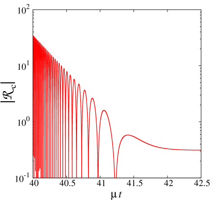
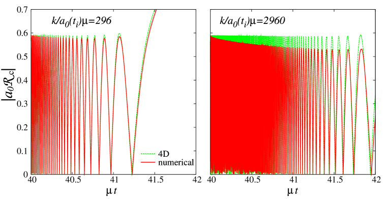
We focus on the dynamics of this quantity. Fig. 1 shows the behaviour of curvature perturbations for $k/\mu=5$ which corresponds to $k/a_{0}(t_{i})\mu\approx 296$. The curvature perturbations ${\cal R}_{c}$ becomes constant on super-horizon scales, which has been shown to be valid even in brane world models [27]. On sub-horizon scales, while ${\cal R}_{c}\propto 1/a_{0}$ in the 4D cosmology, a suppression of the amplitude is observed in the brane-world model, which is due to the coupling to the bulk metric perturbations. In Fig. 2, we compare the amplitude of ${\cal R}_{c}$ obtained in numerical simulations with the one obtained by neglecting the coupling to the bulk metric perturbations, i.e. $J(\Omega)=0$ in Eq. (55). While the difference is very small for the long-wavelength modes (left panel; $k/a_{0}(t_{i})\mu=296$), the suppression becomes significant for the short-wavelength modes (right panel; $k/a_{0}(t_{i})\mu=2960$). Due to this, the spectrum of ${\cal R}_{\rm c}$ just before the horizon crossing acquires a scale dependence as is shown in Fig. 3. Perturbations with larger wavenumber stay on sub-horizon scales for a longer time than those with smaller wavenumber, so they receive more suppression.

Figure 1: The evolution of curvature perturbations ${\cal R}_{c}$ in the inflationary epoch. We set $C=0.1$, $\mu t_{\rm i}=40$ and $k/\mu=5$ which corresponds to $k/a_{0}(t_{i})\mu\approx 296$.

Figure 2: The curvature perturbations (multiplied by the scale factor) in the inflationary epoch for a long-wavelength mode (left; $k/a_{0}(t_{i})\mu\approx 296$) and for a short-wavelength mode (right; $k/a_{0}(t_{i})\mu\approx 2960$). The solid lines represent numerical results and the dashed lines show the 4D predictions obtained by neglecting the coupling to the bulk metric perturbations, that is, by solving Eq. (55) with $J(\Omega)=0$. We set $C=0.1$ and $\mu t_{i}=40$.

Figure 3: The scale dependence of the curvature perturbations evaluated just before the horizon crossing. The horizontal axis represents the physical scale of perturbations evaluated at the initial time $\mu t_{i}=40$. We estimated the ratio $|{\cal R}^{\rm 5D}_{\rm c}/{\cal R}^{\rm 4D}_{\rm c}|$ for each wave number where ${\cal R}^{\rm 5D}_{\rm c}$ is the curvature perturbation in the brane world model and ${\cal R}^{\rm 4D}_{\rm c}$ is the one in a 4D model with the identical background dynamics.

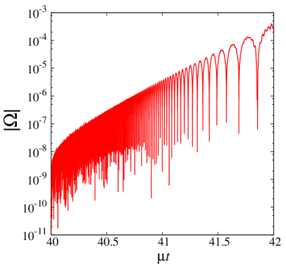
The suppression of the amplitude $\mathcal{R}_{\rm c}$ under horizon may be understood as the excitation of metric perturbations. The suppression of the amplitude of $Q$ is transferred into the enhancement of the metric perturbations $\Omega$ in the bulk, which is shown in the left panel of Fig. 4.

Here we comment on the reason why we evaluated $\mathcal{R}_{\rm c}$ just before the horizon crossing. In the 4D case, we can choose the Bunch-Davis vacuum as an initial condition. Hence we can determine the amplitude and phase of the inflaton perturbations and obtain the spectrum of $\mathcal{R}_{\rm c}$ without any ambiguities. On the contrary, in the present 5D case, the initial conditions cannot be determined without quantising the coupled system. Even in the classical level, the junction condition (58) or (60) restricts our choice of the initial conditions. On superhorizon scales, the initial phase of the perturbations essentially determines its final amplitude after the horizon crossing because the phase determines the amplitude of the growing mode solution on large scales. Then we get an unphysical k-dependence of the curvature perturbations evaluated on superhorizon scales due to the restricted choice of $dQ/dt$ for given $k$. On the other hand, the initial phase is not important when we evaluate the amplitude of the curvature perturbations on small scales. Our aim is to see how $J(\Omega)$ term changes the amplitude of $Q$ in comparison with the 4D solution for various $k$ on small scales. Therefore we chose to calculate the spectrum below the horizon scales.

Figure 4: Left : The bulk metric perturbation $\Omega$ evaluated on the brane. Right : The snapshot of $\Omega$ at $\mu t=41.0$. At this time, the coordinate singularity in the bulk is located at $\mu y_{c}(41.0)\approx 0.34$. We set $C=0.1$, $\mu t_{i}=40$, $k/a_{0}(t_{i})\mu=2960$.

4.3 Check of numerical calculations

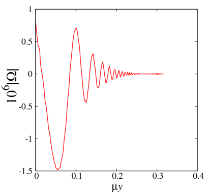
In this section, we first check the assumption of introducing a regulator. As expected from the previous work, $\Omega$ decays fast away from the brane as is shown in the right panel of Fig. 4. This justifies the use of boundary condition $\Omega(y_{\rm reg},t)=0$. In addition, thanks to this behaviour of $\Omega$, the evolution of the curvature perturbations does not depend on the location of the regulator. In fact, even at late times when the information from the regulator brane comes into the brane, the behaviour of the curvature perturbations does not change. Thus our result is not obscured by the regulator brane nor the existence of the coordinate singularity of the GN coordinate.

Finally, we check the accuracy of our numerical simulations by checking the constraint equations derived from the Einstein equations. These equations can be generally expressed as

$$\mathcal{L}(t)\equiv\sum_{k}C_{k}(t)f_{k}(t)=0,$$ (68)

where

$$f_{k}(t)=\{\ddot{\mathcal{R}}_{\rm b},\dot{\mathcal{R}}_{\rm b},\mathcal{R}_{\rm b},\dot{A}_{\rm b},A_{\rm b},\delta\rho_{\mathcal{E}},\delta q_{\mathcal{E}},\delta\pi_{\mathcal{E}}\},$$ (69)

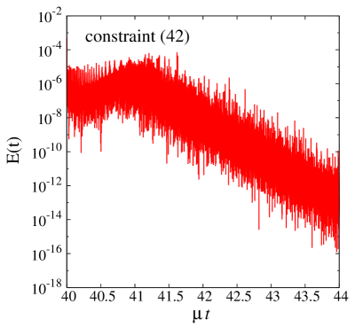
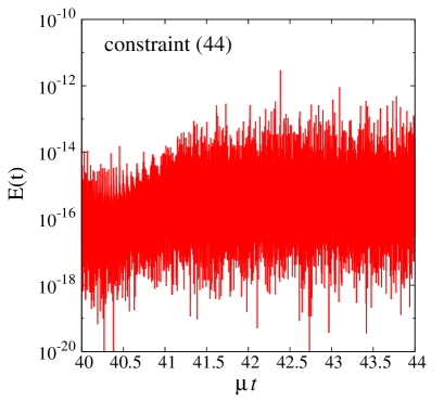
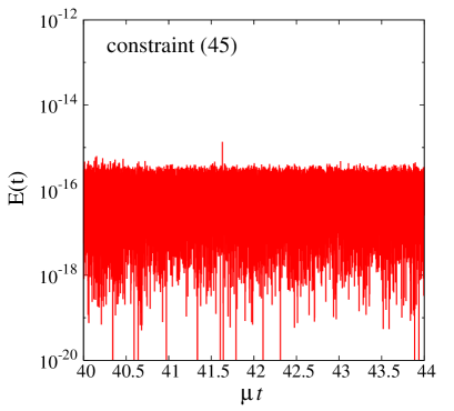
and $C_{k}(t)$ is a set of their coefficients. We calculated the relative error for the constraint equations (42) (44) and (45) as

$$E(t)=\frac{|\mathcal{L}(t)|}{\max_{k}|C_{k}(t)f_{k}(t)|}.$$ (70)

Note that the constraint equation (43) contains higher derivative terms of $\Omega$ like $\ddot{\Omega}^{\prime}$, which are not solved in our simulations. Hence it is impossible to evaluate the numerical accuracy of (43) from our numerical simulation. In fact, if we rewrite the higher-derivative terms of $\Omega$ by $Q$ using Eq. (58), Eq. (43) becomes an identity.

Fig. 5 shows that the relative error of Eq. (42) is suppressed to less than $10^{-5}$ and Eqs. (44) and (45) are very precisely satisfied, indicating that our numerical scheme for solving the coupling system (25) and (55) is reliable. Note that the constraint equation (45) has a different character from the others, which measures the numerical accuracy of the master equation (25) on the brane.

Figure 5: The numerical errors of constraint equations (42)[upper-left], (44)[upper-right] and (45)[lower]. These plots are results of calculations for $k/a_{0}(t_{i})\mu=296$.

5 Conclusion

In this paper, we studied the evolution of the curvature perturbations in a brane-world inflation model where an inflaton is living on a single brane in a 5D AdS spacetime. We used the Hawkins-Lidsey model of the inflaton potential which enables us to derive the background solutions analytically. We solved the full coupled evolution equations for the inflaton perturbations described by the Mukhanov-Sasaki variable and the bulk metric perturbations described by the master variable. This is the first numerical result for the evolution of scalar curvature perturbations in a brane-world that consistently takes into account the backreaction of the metric perturbations.

We used the GN coordinate to describe the bulk spacetime that has a coordinate singularity. Then we are forced to introduce a regulator brane to cut the spacetime. We have checked that the evolution of curvature perturbations is insensitive to the location of the regulator. This is because the bulk metric perturbations decay fast away from the brane. We adopted the simplest possible initial condition for $\Omega$ by taking $\Omega=0$ and $\dot{\Omega}=0$ at an initial time. Then we fix $Q$ so that the boundary condition is consistent. In order to check whether we can consistently neglect the coupling to bulk metric perturbations described by $J(\Omega)$ in Mukhanov-Sasaki equation (55) or not, we followed the subsequent evolution of curvature perturbations numerically.

The evolution of curvature perturbations showed a suppression of the amplitude compared with the conventional 4D model even on sub-horizon scales. This means that it is impossible to neglect a coupling to gravity even on small scales due to the coupling to the higher-dimensional gravity through $J(\Omega)$. The suppression of the amplitude may be understood as a loss of energy due to the excitation of the bulk metric perturbations as we took the initial condition that $\Omega(y,t_{i})=0$ and $\dot{\Omega}(y,t_{i})=0$. On super-horizon scales, the curvature perturbations become constant, which confirms the fact that the constancy of the curvature perturbations is independent of gravitational theory for adiabatic perturbations [27].

Our result suggests that an usual assumption that the inflaton perturbations (the Mukhanov-Sasaki variable) approach to a free massless field on small scales cannot be applied in a brane world models on small scales at high energies. Then the spectrum becomes sensitive to initial conditions not only for the inflaton perturbations but also for bulk metric perturbations. In this sense, we should not take the result Fig. 3 at face value because this result is based on a special choice of initial conditions. In order to determine the initial conditions without ambiguity, it is required to quantise the coupled brane (inflaton)-bulk (metric perturbations) system in a consistent manner along the line of [28]. This is an outstanding open question to be addressed in order to derive the spectrum of the inflaton perturbations in a brane-world.

References

- [1] K. Akama, Lect. Notes Phys., 176, 267 (1982) V.A. Rubakov and M.E. Shaposhnikov, Phys. Lett. B 125 (1983) 136
- [2] D. Langlois, 2003 Prog. Theor. Phys. Suppl. 148 181 [arXiv:hep-th/0209261].
- [3] R. Maartens, 2004 Living Rev. Rel. 7 7.
- [4] P. Brax, C. van de Bruck and A.C. Davis, 2004 Rept. Prog. Phys. 67 2183 [arXiv:hep-th/0404011].
- [5] R. Maartens, D. Wands, B. A. Bassett and I. Heard, 2000 Phys. Rev. D 62 041301 [arXiv:hep-ph/9912464].
- [6] E. Ramirez and A. R. Liddle, 2004 Phys. Rev. D 69 083522 [arXiv:astro-ph/0309608]. D. Seery and A. Taylor, 2005 Phys. Rev. D 71 063508 [arXiv:astro-ph/0309512]; G. Calcagni, 2003 JCAP 0311 009 [arXiv:hep-ph/0310304]; 2004 JCAP 0406 002 [arXiv:hep-ph/0312246].
- [7] A. Liddle and A. N. Taylor, 2002 Phys. Rev. D 65 041301; A. R. Liddle and A. J. Smith, 2003 Phys. Rev. D 68 061301; S. Tsujikawa and A. R. Liddle, 2004 JCAP 0403 001.
- [8] T. Hiramatsu, K. Koyama and A. Taruya, 2004 Phys. Lett. B 578 269 [arXiv:hep-th/0308072]; T. Hiramatsu, K. Koyama and A. Taruya, 2005 Phys. Lett. B 609 133 [arXiv:hep-th/0410247]; T. Kobayashi and T. Tanaka, 2005 Phys. Rev. D 71 124028 [arXiv:hep-th/0505065]. T. Kobayashi and T. Tanaka, 2006 Phys. Rev. D 73 044005 [arXiv:hep-th/0511186]; T. Kobayashi, 2006 Phys. Rev. D 73 124031 [arXiv:hep-th/0602168]; K. Ichiki and K. Nakamura, 2004 Phys. Rev. D 70 064017 [arXiv:hep-th/0310282]; S. S. Seahra, [arXiv:hep-th/0602194].
- [9] T. Hiramatsu, 2006 Phys. Rev. D 73 084008 [arXiv:hep-th/0601105];
- [10] K. Koyama, D. Langlois, R. Maartens and D. Wands, 2004 JCAP 0411 002 [arXiv:hep-th/0408222].
- [11] K. Koyama, S. Mizuno and D. Wands, 2005 JCAP 0508 009 [arXiv:hep-th/0506102].
- [12] C. de Rham, 2005 Phys. Rev. D 71 024015 [arXiv:hep-th/0411021].
- [13] R. M. Hawkins and J. E. Lidsey, 2001 Phys. Rev. D 63 041301 [arXiv:gr-qc/0011060].
- [14] L. Randall and R. Sundrum, 1999 Phys. Rev. Lett. 83 4690.
- [15] T. Shiromizu, K. i. Maeda and M. Sasaki, 2000 Phys. Rev. D 62 024012 [arXiv:gr-qc/9910076].
- [16] P. Binetruy, C. Deffayet, U. Ellwanger and D. Langlois, 2000 Phys. Lett. B 477 285 [arXiv:hep-th/9910219].
- [17] S. Mukohyama, T. Shiromizu and K. i. Maeda, 2000 Phys. Rev. D 62 024028 [arXiv:gr-qc/9912287].
- [18] S. Mukohyama, 2000 Phys. Rev. D 62 084015.
- [19] H. Kodama, A. Ishibashi and O. Seto, 2000 Phys. Rev. D 62 064022.
- [20] D. Langlois, R. Maartens, M. Sasaki and D. Wands, 2001 Phys. Rev. D 63 084009 [arXiv:hep-th/0012044];
- [21] H. A. Bridgman, K. A. Malik and D. Wands, 2002 Phys. Rev. D 65 043502 [arXiv:astro-ph/0107245];
- [22] C. Deffayet, 2002 Phys. Rev. D 66 103504;
- [23] K. Koyama, 2004 JCAP 0409 010 [arXiv:astro-ph/0407263].
- [24] M. Sasaki, 1986 Prog. Theor. Phys. 76 1036; V. F. Mukhanov, 1988 Sov. Phys. JETP 67 1297 [1988 Zh. Eksp. Teor. Fiz. 94N7 1]; V. F. Mukhanov, H. A. Feldman and R. H. Brandenberger, 1992 Phys. Rept. 215 203.
- [25] C. Deffayet, 2005 Phys. Rev. D 71 023520 [arXiv:hep-th/0409302].
- [26] C. Canuto, M. Y. Hussaini, A. Quarteroni and T. A. Zang, 1988 Spectral Methods in Fluid Dynamics, Springer Verlag.
- [27] D. Wands, K. A. Malik, D. H. Lyth and A. R. Liddle, 2000 Phys. Rev. D 62 043527 [arXiv:astro-ph/0003278].
- [28] H. Yoshiguchi and K. Koyama, 2004 Phys. Rev. D 70 043513 [arXiv:hep-th/0403097]; K. Koyama, A. Mennim and D. Wands, 2005 Phys. Rev. D 72 064001 [arXiv:hep-th/0504201].