Towards Inflation and Accelerating Cosmologies
in String-Generated Gravity Models

The string $\alpha^{\prime}$-correction to the usual Einstein action comprises a Gauss-Bonnet integrand multiplied by non-trivial functions of the modulus field $\chi$ and/or the dilaton field $\phi$. We discuss how the presence of such terms in the four dimensional effective action can explain several novel phenomena, such as a four-dimensional flat Friedmann-Robertson-Walker universe undergoing a cosmic inflation at the early epoch, as well as a cosmic acceleration at late times. The model predicts, during inflation, spectra of both density perturbations and gravitational waves that may fall well within the experimental bounds. The model therefore provides a unified approach for explaining the early and late time accelerating phases of the universe.

String/M theory has the prospect of unification of all interactions (see $\!{}^{{\bf?}}$ for a review), providing inter-relationships between quantum mechanics and general relativity. The hope is that the ultimate theory of Nature contains a fundamental and simple, concise relation between close-by and far-away, and past and future. However, string theory, in which great progress was made in the 80’s and 90’s, has not been developed to the stage where the full theory may be employed to construct a detailed cosmology, explaining the evolution of our universe from an epoch near the Planck scale ($\sim{10}^{-33}\,{\rm cm}$) to the presently accessible largest scale ($\sim{10}^{28}\,{\rm cm}$).

The assumptions which make string cosmology a challenging subject are the existence of (yet unobserved) extra dimensions and supersymmetry. Modern (super)string theory or M theory has additional features: it now goes beyond the perturbative approach $\!{}^{{\bf?},{\bf?}}$ popularised in the $80$’s and $90$’s and takes into account the effects due to fluxes, branes, singularities and non-trivial cycles in the extra dimensions. M theory provides new avenues for studying the theory of inflation or cosmic acceleration via flux $\!{}^{{\bf?}}$ or time-dependent $\!{}^{{\bf?}}$ compactifications.

The heterotic string theory after its discovery in 1985 $\!{}^{{\bf?},{\bf?}}$ appeared to be the string theorist’s dream as something like the real world. Only in 1995, there came a breakthrough, not in finding the right version to describe the physical world but in understanding the connections among various versions of string theory, which are related to each other by various string dualities $\!{}^{{\bf?}}$. It is therefore not necessary that all five versions of string theory to be equally relevant in a cosmological context. The four-dimensional effective action of our interest here is given by

$$S=\int d^{4}{x}\sqrt{-g}\bigg{[}\frac{1}{2\kappa^{2}}R-{\gamma}\,(\Delta\chi)^{2}-V(\chi)-\zeta\,(\Delta\phi)^{2}+\frac{1}{8}[\lambda(\phi)-\xi(\chi)]{\cal R}^{2}_{GB}\bigg{]},$$ (1)

where $\kappa$ is the inverse Planck mass $m_{\rm Pl}^{-1}=(8\pi G_{N})^{1/2}$ and ${{\cal R}^{2}_{GB}}\equiv R^{2}-4R_{\mu\nu}R^{\mu\nu}+R_{\mu\nu\rho\chi}R^{\mu\nu\rho\chi}$ is the Gauss-Bonnet (GB) integrand. Here $\phi$ may be viewed as a dilaton, which has no potential, whereas $\chi$ is an ordinary scalar (or inflaton field) which, in particular cases, could be a modulus field associated with the overall size of extra dimensions. In a known example of heterotic string compactification $\!{}^{{\bf?},{\bf?}}$, $\lambda(\phi)=\lambda_{1}\,e^{\phi}+\cdots$ and $\xi(\chi)\propto(\ln(2)-\frac{2\pi}{3}\cosh(\chi))+\cdots$ ($\chi$ is the real part of the common volume modulus). Unfortunately, we do not have a precise knowledge about $V(\chi)$; any such potential may take into account the supersymmetry breaking non-perturbative effects $\!{}^{{\bf?}}$. It may well be that the potential is a function of both $\chi$ and $\phi$, so $V(\chi)\to V(\chi,\phi)$.

Nojiri et al. $\!{}^{{\bf?}}$ examined a special (exact) solution for the system (1) with the choice $V(\chi)=V_{0}\,{\rm e}^{-\chi/\chi_{0}}$ and $\xi(\chi)=\xi_{0}{\rm e}^{\chi/\chi_{0}}$, deleting the $\phi$-dependent terms. The analysis was extended in $\!{}^{{\bf?}}$ (see also $\!{}^{{\bf?}}$) by introducing higher (than second order) curvature corrections, but in the $\chi$=const background. A more general solution, in a fixed dilaton background, $\dot{\phi}=0$, was given in $\!{}^{{\bf?}}$. It was explained there how the model (1) can explain a relaxation of vacuum energy (or effective potential) to a small value (exponentially close to zero) after a sufficiently large number of e-folds of expansion, providing a possible solution to both inflation and cosmological constant problems.

For simplicity, we shall start our discussion by neglecting all the dilaton related terms. We find it convenient to define the following variables (in the units $\kappa=1$):

$$X\equiv{\gamma}\,({\dot{\chi}}/{H})^{2},\quad Y\equiv{V(\chi)}/{H^{2}},\quad U\equiv\xi(\chi)H^{2}\quad\varepsilon\equiv{\dot{H}}/{H^{2}}={H^{\prime}}/{H},$$ (2)

where the dot (prime) denotes a derivative w.r.t. the proper time $t$ (number of e-folds, $N=\int H\,{dt}=\ln(a(t)/a_{0})$). Note that $N$ is a monotonically increasing function of the scale factor, $a(t)$, or the proper time $t$, but its sign depends on the assumption of what the scale $a_{0}$ represents. If $a_{0}$ is the present value of the scale factor, then $N$ is negative in the past, $a(t)<a_{0}$.

In the absence of the Gauss-Bonnet coupling (so $U=0$), the equations of motion are given by $Y=3+\varepsilon$ and $X=-\varepsilon$. These are remarkably simple! However, different choice of $\varepsilon$ implies different $Y$ and hence different $V(\chi)$, and so is the equation of state (EOS) parameter $w$, which is defined by $w=-2\varepsilon/{3}-1$. Is it then all worthy?

In the past, many authors have considered cosmological solutions with various ad hoc choices of the potential, e.g. chaotic potential $V(\chi)=V_{0}+\frac{1}{2}m^{2}\chi^{2}$, exponential potential $V(\chi)=V_{0}\,e^{-p\,\chi}$, inverse power-law potential $V(\chi)=\Lambda^{4}(\chi_{0}/\chi)^{n}$ ($n\geq 2$), the axion-potential $V(\chi)=\Lambda^{4}(c\pm\cos(\chi/\chi_{0}))$, and so on. The models with exponential and inverse power-law potentials possess some interesting features at late times, such as the cosmological attractors $\!{}^{{\bf?},{\bf?}}$. Though it may be desirable to construct a cosmological model that gives rise to

$$w\approx-1,$$ (3)

for the model to work, the field $\chi$ must relax its potential energy after inflation down to a sufficiently low value, possibly very close to the present value of dark energy, $\Lambda_{vac}\sim(10^{-3}\,{\text{eV}})^{4}$. Do all of the above potentials possess such feature? The answer is soundly no! An exponential potential is perhaps the best choice but it is more plausible that the coupling constant $p$ is a function of the field $\chi$ itself, or the number of e-folds, $N\equiv|\ln(a_{f}/a_{i})|$.

For generality, we assume that $\xi(\chi)\neq 0$, without specifying its sign at this stage. In an accelerating universe, the Gauss-Bonnet term is positive, i.e., ${\cal R}_{GB}^{2}=24\frac{\dot{a}^{2}\ddot{a}}{a^{3}}>0$. The effective potential, which may be given by $\Lambda(\chi)\equiv V(\chi)-\frac{1}{8}\,\xi(\chi)R_{GB}^{2}$, can be (exponentially) small for $V(\chi)\approx\frac{1}{8}\,\xi(\chi)R_{GB}^{2}$. We find it convenient to impose the condition $\!{}^{{\bf?},{\bf?}}$

$$\Lambda(\chi)\equiv H^{2}(3+\varepsilon),$$ (4)

so that $\Lambda(\chi)\geq 0$ for $\varepsilon\geq-3$ or equivalently when the EOS parameter $w\leq 1$. There is now only one free parameter in the model, which may be fixed either by allowing one of the variables in (2) to take a fixed (but arbitrary) value or by making an appropriate ansatz. Here we consider two physically motivated cases. First consider the case of power-law inflation, for which

$$a(t)\equiv e^{\omega(t)}\equiv\left(c_{0}t+t_{1}\right)^{-1/\varepsilon_{0}},$$ (5)

where $c_{0}$ and $t_{1}$ are arbitrary constants. This actually implies that $\varepsilon\equiv\dot{H}/H^{2}=\varepsilon_{0}$. For $\varepsilon_{0}<0$, $c_{0}>0$ and $t_{1}$ may be set zero, but, for $\varepsilon_{0}>0$, one may take $c_{0}<0$ and set $t_{1}=t_{\infty}$, just to ensure that the scale factor grows with $t$ in either case. With (5), we find $H\propto e^{\varepsilon_{0}N}$ and $\xi(\chi)H^{2}=c_{2}\,e^{\alpha_{+}N}+c_{3}\,e^{\alpha_{-}N}$, where $\alpha_{\pm}=\frac{1}{2}\left(\varepsilon_{0}-5\pm\sqrt{9(\varepsilon_{0}+3)^{2}-32}\right)$. For the reality of $\alpha_{\pm}$, it is required that $\varepsilon_{0}>-1.11$ or $\varepsilon_{0}<-4.88$; we rule out the latter as it implies $w>1$.

Spurred on by this example, we make no assumption about the form of scale factor, and instead consider the ansatz that during a given epoch we may make the approximation

$$U\equiv\xi(\chi)H^{2}\equiv e^{\alpha_{0}+\alpha N},$$ (6)

where $\alpha_{0}$ and $\alpha$ are arbitrary at this stage. This allows us to write $\varepsilon$ in a closed form:

$$\varepsilon=\beta\tanh\beta(N+N_{1})-\hat{\beta}\quad\Rightarrow H\propto\cosh\beta(N+N_{1})\,e^{-\hat{\beta}\,N},$$ (7)

where $N_{1}$ is a free parameter, $\hat{\beta}\equiv(16+\alpha)/{4}$ and $\beta\equiv\frac{1}{4}\,\sqrt{9\alpha(\alpha+8)+208}$. Initially, $N$ may take a large negative value, $N\equiv\ln(a/a_{0})\ll 0$. As we wish to obtain an inflationary epoch with sufficiently large number of e-folds of expansion, say $65$ e-folds, it is reasonable to take $N_{1}\sim{\cal O}(65)$. For $\Delta N\equiv N+N_{1}\lesssim 0$, the universe is not accelerating, but it starts to accelerate ($\varepsilon>-1$) for $\Delta N\gtrsim 0.2$. The solution where $-6<\alpha<-4$ (or $-2<\alpha<1$) is accelerating with the EOS parameter $w\geq-1$; of course, the solution where $\alpha<-6$ (or $\alpha>1$) is also accelerating but in this case, since $\varepsilon>0$ or $X<0$ (cf figure 1), $\chi$ may behaves as a phantom field.

The scalar field potential may be given by

$$V(\chi)=H^{2}\left(3+\varepsilon+3(\varepsilon+1)U\right).$$ (8)

Note that at the start of inflation, $\varepsilon\approx-1$ (or $w\approx-1/3$), the GB term is not contributing; inflation can be mainly due to the potential. One may express (8) in terms of the scalar field $\chi$, although it involves a somewhat complicated relation between $N$ and $\chi$, namely,

$$\gamma{\chi^{\prime}}^{\,2}=-\frac{1}{2}\left[\alpha(\alpha-1)-2({\hat{\beta}}^{2}+\beta^{2})+(\alpha-2)\hat{\beta}+(2\beta-\alpha\beta+4\hat{\beta}\beta)\tanh(\beta\Delta N)\right]U$$

$$\quad+\,\hat{\beta}-\beta\tanh(\beta\Delta N).$$ (9)

After a certain number of e-folds of expansion, i.e., $\beta\Delta N\gtrsim 2$, this simplifies to

$$\gamma{\chi^{\prime}}^{\,2}\to\frac{e^{\alpha_{0}}}{2}(\alpha+2\hat{\beta}-2\beta)(1-\alpha+\hat{\beta}-\beta)e^{\alpha N}+\hat{\beta}-\beta\equiv x_{0}(\alpha)$$ (10)

Especially, for $\alpha=1$, we get $\hat{\beta}=\beta$ and hence $\chi^{\prime}\simeq 0$ when $\beta\Delta N\gtrsim 2$, i.e., the time-variation of the field $\chi$ or its rolling with $N$ is negligibly small. In this case $\Lambda(\chi)$ acts purely as a cosmological constant term. Note that $\hat{\beta}=\beta$ is obtained also for $\alpha=-6$, but in this case $\chi$ may behave as a phantom field unless $\xi(\chi)$ is chosen to be negative or the coefficient $e^{\alpha_{0}}$ is exponentially small, $\alpha_{0}\to-\infty$. In the limit $U\ll 1$, so that the Gauss-Bonnet correction is small and is not dominating the dynamics, the potential is well approximated by $V(\chi)\propto H^{2}\propto e^{2(\beta-\hat{\beta})N}\equiv V_{0}\,e^{-p\,\chi}$ where $p\equiv 2(\hat{\beta}-\beta)\lambda_{0}$ and $\lambda_{0}=\sqrt{\frac{\gamma}{x_{0}(\alpha)}}=|\chi^{\prime}|_{\beta\Delta N>2}$. Furthermore, we get $\Lambda(\chi)=\Lambda_{0}\,e^{-p\,\chi}$, which is valid for any value of $\alpha$ (or $N$) but satisfying $\beta\Delta N>2$.

Figure 1: The $\Delta N$ - $\alpha$ phase space. The almost horizontal line with $\varepsilon=-3$ separates the regions between $\Lambda(\chi)>0$ and $\Lambda(\chi)<0$. Here we have set ${\alpha_{0}}=\ln(0.5)$. The region with $\varepsilon<-3$ (or $\Lambda(\chi)<0$) is physically less relevant as it implies $w>1$. Only the lines with $\varepsilon>-1$ fall in the accelerating region. For $-6\leq\alpha\leq-4$, $V(\chi)$ is always non-negative; $V(\sigma)\geq 0$ may be required in order that the vacuum becomes a possible ground state.

For a canonically normalized field $\chi$ such that $K(\chi)=\frac{1}{2}\dot{\chi}^{\,2}$, the exponential potential $\Lambda=\Lambda_{0}\,e^{-p\,\chi}$ with $p=p(\chi)$ possesses some interesting cosmological features $\!{}^{{\bf?}}$, which are unavailable if $p$ is a constant. Notably, one would require $p<\sqrt{2}$ to obtain an inflationary solution, where as $p>\sqrt{6}$ may be required after inflation in order for the potential energy not to dominate the energy content of the universe, satisfying the necleosynthesis bound, namely $p^{2}>n/{\Omega_{\chi}^{\rm max}}$, where $n=3$ ($4$) for matter (radiation). The nucleosysthesis bound is not violated for $(\hat{\beta}-\beta)\lambda_{0}\gtrsim\sqrt{5}$, given that $\Omega_{\chi}^{\rm max}\lesssim 0.2$. Though the model studied in $\!{}^{{\bf?}}$, namely, $V(\chi)=\Lambda^{4}\left(e^{-\,P\chi}+e^{-\,Q\chi}\right)$, did not work satisfactorily, as it required $P>5.5$ (and $Q<0.8$) in order to satisfy a constraint coming from the nucleosynthesis bounds on $\Omega_{\chi}$, a scalar potential as a sum of two (or more) exponential terms of different slopes may be interesting from some other reasons, for example, it gives rise to more than one period of cosmic acceleration $\!{}^{{\bf?},{\bf?}}$.

Let us now return to the discussion related to (7). The scale factor of the universe after inflation would naturally become much larger than its initial value, but it is smaller than $a_{0}$, i.e. the present value, so $-{\cal O}(1)\lesssim N<0$. Our approximation (6) that $U$ be given by a single exponential term may break down at some intermediate epoch (cf Fig 2). Sometime later, $U$ may be approximated by the term $\propto e^{\hat{\alpha}N}$. The solution is then given by (7), with $\alpha$ and $N_{1}$ replaced by $\hat{\alpha}$ and $N_{0}$, respectively. For $N+N_{0}\lesssim 0$, the universe is in a deceleration phase which implies that inflation must have stopped during the intermediate epoch. As $N$ crosses $N_{0}$, or when $N+N_{0}>0$, the universe may begin to accelerate for the second time.

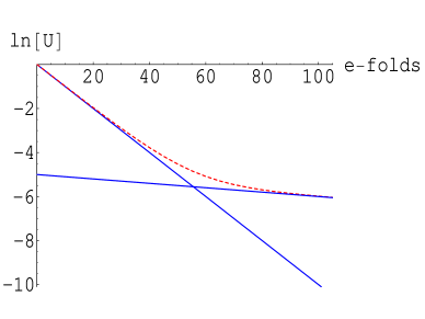
Figure 2: The qualitative behavior of the product $\xi(\chi)H^{2}\equiv U(\chi)=e^{\alpha_{0}+\alpha N}+e^{\alpha_{1}+\hat{\alpha}N}$ (dotted line) as a function of the number of e-folds, with $\alpha=-0.1$, $\hat{\alpha}=-0.01$, $\alpha_{0}=0$ and $\alpha_{1}=-5$. The time-variation of the coupling function $U(\chi)$ may be large at early times (before the end of inflation), but it is nearly constant at late times.

For $a(t)\sim a_{0}$, we get $N\sim 0$ and hence $\Delta\chi\propto\Delta N$; the constant of proportionality may be small. This implies that, after inflation, even if $\hat{\alpha}$ is very different from unity, the time-variation of $\chi$ may be small, unless we do not demand a large number of e-folds of expansion. It is also possible that after inflation the field $\chi$ stabilises (i.e. no significant rolling with $N$) and the late time acceleration is due to slow rolling of the field $\phi$. Later we will discuss about this possibility. Below we discuss the result of cosmological perturbations for a single scalar field $\chi$.

It is generally believed that during inflation the inflaton and graviton field undergo quantum-mechanical fluctuations $\!{}^{{\bf?}}$, leading to scalar (density) and tensor (gravity waves) fluctuations, which in turn would give rise to significant effects on the large-scale structures of the universe at the present epoch. In turn, it may be hoped that the spectra of perturbations provide a potentially powerful test of the inflationary hypothesis. In this respect, one may ask whether the solution of the type (7) can generate scalar perturbations of the desired magnitudes, like $\delta_{H}\equiv\delta\rho/\rho\sim 2\times{10}^{-5}$ and $n\simeq 0.95$. The spectral index (or tilt parameter) is given by

$$n\simeq 1-4\epsilon+2\eta,$$ (11)

where $\epsilon\equiv 2(\ln H)^{\prime}/{\chi^{\prime}}^{\,2}$ and $\eta\equiv 2\left[H^{\prime\prime}/H-(\ln H)^{\prime}(\ln\chi^{\prime})^{\prime}\right]/{\chi^{\prime}}^{\,2}$. We note that inflationary predictions with $\xi(\chi)\neq 0$ can be significantly different from those with $\xi(\chi)=0$ (see $\!{}^{{\bf?}}$ for discussions on the related theme). In our model, a spectral index of magnitude $n\simeq 0.95$ may be obtained with $\alpha\simeq-5.964$ or with $\alpha\sim[-0.04,0.04]$ (cf figure 3). Furthermore, for $\alpha\approx-6$ and $\alpha\gtrsim 0$, the tensor-to-scalar ratio may be negligibly small, $r\equiv A_{T}/A_{S}\ll 0.4$ $\!{}^{{\bf?}}$.

Figure 3: The contour plot of $\alpha$ and $u$ ($\equiv\exp(\alpha_{0})$), showing the value of the spectral index $n=1-4\epsilon+2\eta$ in the range $[0.93,0.97]$; $n$ is independent of the value of $u$ for a large negative value of $\alpha$ ($<-4$)

The acceleration of the universe at late times $\!{}^{{\bf?}}$ is a surprising and enormously influential result. It is worthwhile to know if the dilaton plays a special role in the present accelerated phase of the universe. So far we discussed the result with no $\phi$-dependent terms in the action, or that $\dot{\phi}\simeq 0$. In the presence of $\phi$-dependent terms, one may introduce two more variables:

$$\Phi\equiv\lambda(\phi)H^{2},\quad W\equiv\zeta\,({\dot{\phi}}/{H})^{2}.$$ (12)

First consider the case $\zeta=0$, for which there is no kinetic term for $\phi$. $\Phi$ is assumed to be positive; of course, its time variation must be small at late times so as not to conflict with ground based solar system tests of GR. Here we do not impose any condition like (4). Especially, for $U=\Phi$, for which $\phi$ is behaving similarly as $\chi$ and hence $f\equiv\lambda(\phi)-\xi(\chi)=0$, we find $\!{}^{{\bf?}}$

$$X=-(\ln U)^{\prime},\quad Y=3+(\ln U)^{\prime}/2,\quad\varepsilon=(\ln U)^{\prime}/2.$$ (13)

The solution $U\propto e^{\alpha N}$ leads to an accelerated expansion of the universe for $\alpha>-2$; in particular, for $\alpha=-0.09$, we get $\varepsilon=-0.045$ and hence $w=-0.97$. According to the recent WMAP result $\!{}^{{\bf?}}$, putting together all the experiments, the measured value of the dark energy EOS parameter is $w_{DE}=-\,1.06_{-\,0.08}^{+\,0.13}$. For the above solution, it is required that $\alpha=0.18_{+\,0.24}^{-\,0.39}$. Especially, for $\alpha=0$, the effect is similar to that of a cosmological constant term, $w_{\Lambda}=-1$.

In the case $\zeta\neq 0$, the field equations are solved explicitly, for example, with $U=\Phi={\rm const}\equiv\Phi_{0}$. Then, there exist three branches of solution: the first branch is given by $\varepsilon=\sqrt{6}\tanh(\sqrt{6}(N+N_{0}))-3$ and $W=-3\Phi_{0}(1+2\varepsilon)$. For this solution the universe enters into an accelerating phase for $N+N_{0}\gtrsim 0.22$. In particular, for $N+N_{0}\gtrsim 2$, the deceleration parameter $q$ is almost constant, $q\equiv-\,a\ddot{a}/{\dot{a}}^{2}=-1-\varepsilon\simeq 0-0.45$. Furthermore, we get $W\simeq 0.3\Phi_{0}$, so that, for $\Phi_{0}>0$, $\phi$ behaves as a canonical scalar. Either both of the other two branches support an accelerating phase with $w>-1$, or only one of the branches supports inflation with $w<-1$.

Finally consider a situation near the analytic minimum where $V(\chi)\simeq 0$. In this case a cosmic acceleration at late times may arise due to slow rolling of the field $\phi$ and/or $\xi$:

$$\dot{\chi}\equiv\sqrt{\frac{|\chi_{0}|}{\gamma}}\,H,\quad\dot{\phi}=\sqrt{\frac{|\phi_{0}|}{\zeta}}\,H\left(\frac{a_{0}}{a}\right)^{m/2}\equiv\sqrt{\frac{|\phi_{o}|}{\zeta}}\,H\,e^{-mN/2},$$ (14)

where $\chi_{0}$, $\phi_{0}$ and $m$ are arbitrary at this stage. The solution is given by

$$\Xi\equiv\dot{\chi}H\frac{d\xi(\chi)}{d\chi}=\frac{4\chi_{0}(\chi_{0}-3)+2\chi_{0}\phi_{0}(m-2)e^{-mN}}{3\left(4\chi_{0}+(4-m)\phi_{0}\,e^{-mN}\right)},$$

$$\Psi\equiv\dot{\phi}H\frac{d\lambda(\phi)}{d\phi}=\frac{1}{3}\,\frac{(m+4)\chi_{0}\phi_{0}+(m-4){\phi_{0}}^{2}\left(3-e^{-mN}\right)}{4\chi_{0}\,e^{mN}+(4-m)\phi_{0}},$$

$$\varepsilon=-1+\frac{(m-4)\phi_{0}\,e^{-mN}-4\chi_{0}}{3+\chi_{0}+\phi_{0}\,e^{-mN}}.$$ (15)

The solution may be modelled such that $\ln(1+z)=|\Delta N|=\ln(a_{f}/a_{i})$, where $z$ is the red-shift factor. The number of e-folds $\Delta N\sim 0.7$ when $z$ drops from $1$ to $0$. For simplicity, let us assume that $\chi_{0}\simeq 0$, so that $\chi$ stabilises. Then the solution (Towards Inflation and Accelerating Cosmologies in String-Generated Gravity Models) can support a transition between phantom-like phase ($\varepsilon>0$) and standard (non-phantom) phase ($\varepsilon<0$), especially, for $m\geq 5$. However, if $\phi$ stabilises ($\dot{\phi}=0$) before $\chi$ stabilises, then we find $\varepsilon\simeq-1-4\chi_{0}/(3+\chi_{0})$; with $\chi_{0}>0$, as such the case for a canonical $\chi$, the solution is not accelerating since $\varepsilon>-1$. However, if both scalars $\phi$ and $\chi$ are (slowly) rolling with time, it is possible that the EOS parameter $w<-1/3$, although its value is more sensitive to the choice of the parameters $\chi_{0}$ and $\phi_{0}$.

In summary, we have shown that the string $\alpha^{\prime}$-correction to the usual gravitational action of general relativity of the Gauss-Bonnet form plays an important and interesting role in explaining the early and late time accelerating phases of the universe, with singularity-free solutions. For constant dilaton phase of the standard scenario, the model can predict during inflation spectra of both density perturbations and gravitational waves that may fall well within the experimental bounds. It is hoped that the results in this paper help for explaining both the inflation and the cosmic acceleration at late times. For completeness, in particular, in order to study the transition between deceleration and acceleration, one may have to include matter field which is also the constituent that we know dominates the universe during deceleration (see $\!{}^{{\bf?}}$ for a work in this direction). In the presence of a barotropic fluid (matter/radiation), one defines an effective EOS parameter, $w_{eff}$, which may differ from the $w$ obeyed by a source of dark energy alone, like the scalar potential, $V(\chi)$, or by some exotic source of dark energy such as K-inflaton.

Acknowledgement This work was supported in part by the Marsden fund of the Royal Society of New Zealand. I acknowledge helpful discussions and e-mail correspondences with Shin’ichi Nojiri, Sergei Odintsov and M. Sami during the course of this project.

References

References

- [1] K.R. Dienes, Phys. Rept. 287, 447 (1997).
- [2] P. Candelas, G. T. Horowitz, A. Strominger and E. Witten, Nucl. Phys. B 258, 46 (1985).
- [3] D. J. Gross, J. A. Harvey, E. J. Martinec and R. Rohm, Phys. Rev. Lett. 54, 502 (1985).
- [4] S. Kachru, R. Kallosh, A. Linde and S. P. Trivedi, Phys. Rev. D 68, 046005 (2003).
-
[5]
C.M. Chen, P.M. Ho, I.P. Neupane, N. Ohta and J. Wang,
JHEP 0310, 058 (2003);
K. i. Maeda and N. Ohta,
Phys. Rev. D 71, 063520 (2005);
I.P. Neupane and D. L. Wiltshire, Phys. Lett. B 619, 201 (2005); ibid Phys. Rev. D 72, 083509 (2005). - [6] A. Sen, Nucl. Phys. Proc. Suppl. 58, 5 (1997).
- [7] I. Antoniadis, E. Gava and K. S. Narain, Phys. Lett. B 283, 209 (1992).
- [8] I. Antoniadis, J. Rizos and K. Tamvakis, Nucl. Phys. B 415, 497 (1994).
- [9] S. Nojiri, S.D. Odintsov and M. Sasaki, Phys. Rev. D 71, 123509 (2005).
- [10] M. Sami, A. Toporensky, P.V. Tretjakov and S. Tsujikawa, Phys. Lett. B 619, 193 (2005).
- [11] G. Calcagni, S. Tsujikawa and M. Sami, Class. Quant. Grav. 22, 3977 (2005).
- [12] I.P. Neupane and B.M.N. Carter, hep-th/0510109 (to appear in PLB).
-
[13]
P.G. Ferreira and M. Joyce,
Phys. Rev. Lett. 79, 4740 (1997);
E.J. Copeland, A.R. Liddle and D. Wands, Phys. Rev. D 57, 4686 (1998). - [14] P.J. Steinhardt, L.M. Wang and I. Zlatev, Phys. Rev. D 59, 123504 (1999).
- [15] I.P. Neupane and B.M.N. Carter, hep-th/0512262 (to appear in JCAP).
- [16] H. Tashiro, T. Chiba and M. Sasaki, Class. Quant. Grav. 21, 1761 (2004).
- [17] T. Barreiro, E.J. Copeland and N.J. Nunes, Phys. Rev. D 61, 127301 (2000).
-
[18]
I.P. Neupane,
Class. Quant. Grav. 21, 4383 (2004); ibid
Mod. Phys. Lett. A 19, 1093 (2004);
L. Jarv, T. Mohaupt and F. Saueressig,
JCAP 0408, 016 (2004);
F.C. Carvalho and A. Saa, Phys. Rev. D 70, 087302 (2004). -
[19]
A.D. Linde,
Phys. Lett. B 116, 335 (1982);
A.A. Starobinsky, Phys. Lett. B 117, 175 (1982);
V.F. Mukhanov, H.A. Feldman and R.H. Brandenberger, Phys. Rept. 215, 203 (1992); E.D. Stewart and D.H. Lyth, Phys. Lett. B 302, 171 (1993). -
[20]
J.c. Hwang and H. Noh,
Phys. Rev. D 61, 043511 (2000);
C. Cartier, J.c. Hwang and E.J. Copeland, Phys. Rev. D 64, 103504 (2001);
S. Tsujikawa, R. Brandenberger and F. Finelli, Phys. Rev. D 66, 083513 (2002). -
[21]
C.L. Bennett et al,
Astrophys. J. Suppl. 148, 1 (2003);
D.N. Spergel et al [WMAP Collaboration], Astrophys. J. Suppl. 148, 175 (2003);
A.G. Riess et al [Supernova Search Team Collaboration], Astrophys. J. 607, 665 (2004). - [22] I.P. Neupane, hep-th/0602097.
-
[23]
D.N. Spergel et al, astro-ph/0603449;
http://lambda.gsfc.nasa.gov/product/map/dr2/params/ocdm-w-all.cfm - [24] B. McInnes, Nucl. Phys. B 718, 55 (2005).
- [25] S. Nojiri and S.D. Odintsov, Phys. Lett. B 631, 1 (2005).
- [26] I.Y. Aref’eva and A.S. Koshelev, hep-th/0605085.
- [27] L. Perivolaropoulos, JCAP 0510, 001 (2005); I. Brevik, gr-qc/0601100.
-
[28]
H. Wei and R.G. Cai,
Phys. Lett. B 634, 9 (2006);
Z.G. Huang, H.Q. Lu and W. Fang, hep-th/0604160. - [29] S. Nojiri, S.D. Odintsov and M. Sami, hep-th/0605039.