Bulk Singularities and the Effective Cosmological Constant
for Higher Co-dimension Branes

Abstract

We study a general configuration of parallel branes having co-dimension $\geq 2$ situated inside a compact $d$-dimensional bulk space within the framework of a scalar and flux field coupled to gravity in $D$ dimensions, such as arises in the bosonic part of some $D$-dimensional supergravities. A general relation is derived which relates the induced curvature of the observable noncompact $n$ dimensions to the asymptotic behaviour of the bulk fields near the brane positions. For compactifications down to $n=D-d$ dimensions we explicitly solve the bulk field equations to obtain the near-brane asymptotics, and by so doing relate the $n$-dimensional induced curvature to physical near-brane properties. In the special case where the bulk geometry remains nonsingular (or only conically singular) at the brane positions our analysis shows that the resulting $n$ dimensions must be flat. As an application of these results we specialize to $n=4$ and $D=6$ and derive a new class of solutions to chiral 6D supergravity for which the noncompact 4 dimensions have de Sitter or anti-de Sitter geometry.

I Introduction

In four dimensions the twin requirements of general covariance and the Lorentz-invariance of the vacuum imply that the vacuum energy inevitably appears to gravity like a 4D cosmological constant, with a vacuum energy, $\rho$, corresponding to a cosmological constant of order $\Lambda=8\pi G\rho$ (where $G$ here denotes Newton’s constant). The cosmological constant problem ccreview refers to the huge mismatch between the large vacuum energy expected from the known quantum zero-point fluctuations and the very small upper limit on (or the observed value for) the cosmological constant coming from cosmology.

Higher dimensional theories are of interest for the cosmological constant problem because they offer the possibility that the gravitational influence of a 4D vacuum energy need not be a 4D cosmological constant. In particular, within a higher-dimensional context the possibility exists that the gravitational response of a large 4D vacuum energy might be to curve the extra dimensions rather than the observable four, raising the hope that a large vacuum energy need not lead to a large 4D cosmological constant. The introduction of branes into the picture considerably sharpens this hope, since solutions exist to the higher-dimensional field equations for which the effective 4D cosmological constant vanishes even though they are sourced by large 4D energy configurations (typically large brane tensions).

In recent years these observations have stimulated several proposals to realize this possibility in a concrete way precursors ; codim1 ; carroll ; sled , all with the theme that large 4D energy densities need not imply a strongly-curved 4D geometry within a brane-world picture. Although this is arguably a step forward, it is not the end of the story since the mere existence of such solutions does not directly address the issues of fine-tuning which underly the cosmological constant problem. These issues come in several forms, either to do with the stability of the solution under the quantum renormalization of the underlying parameters, or to do with stability of the time evolution of the solutions against perturbations in the initial conditions (for a review of some of these concerns see TAMU ).

One of the key questions underlying these naturalness issues asks: What conditions must be required of the various source brane configurations in order to make the observed 4 dimensions flat? This question is crucial for addressing the fine-tuning issue because one must always be on guard against hidden fine tunings. In particular, if the properties of various branes must be carefully adjusted (or adjusted relative to one another) then it is the stability of this particular adjustment (against renormalization, say) which must be established in order to solve the cosmological constant problem. Indeed the main criticisms to proposals precursors ; codim1 ; carroll ; sled fall into this category codim1x ; carrollx ; sledx (see also TAMU ; update ).

It is our purpose in this paper to provide a general answer to this question for a scalar-tensor-flux field equations arising in $D$-dimensional supergravity theories, for solutions having $n$ maximally-symmetric dimensions that are sourced by branes having co-dimension $\geq 2$. (The case of co-dimension 1 – as appropriate for Randall-Sundrum models RS , for instance – differs from other co-dimensions and is presently better understood codim1x .) We defer to a later paper the discussion of the naturalness issues associated with the quantum corrections to, and the stability of, the solutions presented here.

For these systems we obtain the following results:

• We derive a general expression, eq. (8), which relates (a particular average over the extra dimensions of) the curvature of the maximally-symmetric $n$ dimensions to the asymptotic form taken by the bulk metric very close to the source branes. Our expression generalizes similar expressions which have been derived, either for 6D supergravities in the co-dimension 2 case GGP or for higher-dimensional non-supersymmetric gravity ML . Our result also applies to FRW-like time-dependent geometries for which the $n$ maximally-symmetric dimensions are spatial, in which case the spatial curvature is related to both the near-brane asymptotic forms and to contributions from spatial slices in the remote past and future.

• We provide a very general classification of the near-brane form taken by the bulk fields near their sources. Using arguments in the spirit of the BKL analysis of time-dependence near singularities BKL we show that in the near-brane limit the higher-dimensional supergravity fields have a power-law dependence on the proper distance, $r$, from the branes. We show that the bulk fields are very generically singular near the branes, and that the bulk field equations impose Kasner-like relations, eqs. (17) and (19), amongst these powers, which strongly restrict the kinds of powers (and so also the singularities) which arise.

• Combining the above two points allows an identification of how the curvature of the large $n$ dimensions depends on the asymptotic powers which govern the asymptotic near-brane behaviour of the bulk fields. This relation shows that the large $n$ dimensions must be flat in the absence of singularities within the extra dimensions (or if these singularities are only conical). In the more generic case of singular configurations we find that a flat $n$ dimensions requires either the extra-dimensional warp factor, $W$, or the dilaton, $e^{\varphi}$, must grow like an inverse power of $r$ as the brane is approached (i.e. as $r\to 0$). (In our conventions $e^{\varphi}\ll 1$ corresponds to weak coupling in string theory.)

• As an application we specialize the above results to the case of 6D supergravity compactified to 4 dimensions, and use them to show the existence of a new class of solutions for which the maximally-symmetric 4 dimensions are de Sitter-like (or anti-de Sitter-like), unlike all of those which are presently known.

Our presentation is organized in the following way. The next section sets up the supergravity equations of interest and their compactification to $n$ maximally-symmetric dimensions. It is here that we derive the key relationship, eq. (8), relating the $n$-dimensional curvature to the asymptotics of bulk fields near the source-brane singularities. Section III then examines the relevant near-brane asymptotic forms for the bulk fields, and derives the power-law behaviour which the bulk equations dictate. These are then used in the results of Section II to more directly relate the $n$-dimensional curvature to the power-law dependence of the bulk fields in the near-brane limit. Finally, Section IV specializes to 6D supergravity compactified to 4 maximally-symmetric dimensions, and shows how to use the previous two sections to generalize the class of 6D solutions to include those having de Sitter-like and anti-de Sitter-like 4-dimensional slices.

II The Curvature-Asymptotics Connection

In this section we summarize the field equations of interest, which are the bosonic parts of the equations of motion for many higher-dimensional supergravities. We also here specialize the fields appearing in these equations to the most general configurations which are maximally symmetric in (3+1) non-compact dimensions, as is appropriate for describing the warped compactifications of interest. We allow these solutions to have singularities (more about which below) at various points within the extra dimensions corresponding to the positions of various branes having co-dimension $\geq 2$. Our goal in so doing is to establish a general connection, eq. (8), between the curvature of the noncompact 4D geometry and the asymptotic behaviour of the bulk fields in the vicinity of the various branes.

II.1 The Field Equations

Our starting point is the following action in $D$ spacetime dimensions

$$S=-\int{\rm d}^{D}x\sqrt{-g}\left[\frac{1}{2\kappa^{2}}\,g^{MN}\Bigl{(}R_{MN}+\partial_{M}\varphi\,\partial_{N}\varphi\Bigr{)}+\frac{1}{2}\sum_{r}\frac{1}{(p_{r}+1)!}e^{-p_{r}\varphi}F_{r}^{2}+{\cal A}\,e^{\varphi}\right]\,,$$ (1)

where $\kappa^{2}=8\pi G$ denotes the higher-dimensional Newton constant and ${\cal A}$ is a dimensional constant. The fields $F_{r}$ are the $(p_{r}+1)$-form field strengths for a collection of $p_{r}$-form gauge potentials, $A_{r}$, and $F^{2}=F_{M_{1}..M_{p_{r}+1}}F^{M_{1}..M_{p_{r}+1}}$. When ${\cal A}=0$ this is sufficiently general to encompass the bosonic parts of a variety of higher-dimensional, ungauged supergravity lagrangian densities HiDSugra . When ${\cal A}\neq 0$ the dilaton potential has the form found in chiral 6D supergravity NS .

The field equations obtained from this action are:

$$\Box\,\varphi-\kappa^{2}{\cal A}\,e^{\varphi}+\kappa^{2}\sum_{r}\frac{p_{r}}{2(p_{r}+1)!}e^{-p_{r}\varphi}F_{r}^{2}=0\qquad\hbox{(dilaton)}$$

$$\nabla_{M}\Bigl{(}e^{-p_{r}\varphi}\,F_{r}^{MN\ldots Q}\Bigr{)}+(\hbox{CS terms})=0\qquad\hbox{($p_{r}$-form)}$$ (2)

$$R_{MN}+\partial_{M}\varphi\,\partial_{N}\varphi+\kappa^{2}\sum_{r}\frac{1}{p_{r}!}e^{-p_{r}\varphi}\left[F_{r}^{2}\right]_{MN}+\frac{2}{D-2}\,(\Box\,\varphi)\,g_{MN}=0\qquad\hbox{(Einstein)}\,,$$

where ‘(CS terms)’ denotes terms arising from any Chern-Simons terms within the definition of $F_{(r)}$, and we define

$$\left[F^{2}\right]_{MN}=F^{\hskip 7.0ptP\ldots R}_{M}F_{NP\ldots R}\,.$$ (3)

The ability to write the term proportional to $g_{MN}$ in the Einstein equation in terms of $\Box\varphi$ is a consequence of the particular powers of $e^{\varphi}$ which pre-multiply each of the terms in the action, (1). This choice corresponds to the existence of a scaling symmetry of the classical field equations, according to which

$$g_{MN}\to\omega\,g_{MN}\quad\hbox{and}\quad e^{\varphi}\to\omega^{-1}\,e^{\varphi}\,,$$ (4)

with constant $\omega$ and the field strengths, $F_{r}$, not transforming. Although this is not a symmetry of the action, which transforms as $S\to\omega^{(D-2)/2}S$, it does take solutions of the classical equations into one another.

II.2 Maximally-Symmetric Compactifications

We seek solutions to these equations for which $n$ dimensions are maximally symmetric and $d=D-n$ are not. In most applications we have in mind $n=4$, corresponding to having 3+1 maximally-symmetric directions and $d=D-4$ static, compact euclidean dimensions. But our analysis is general enough also to include (with minor modifications) situations of interest to cosmology for which there are $n=3$ maximally-symmetric spatial dimensions and $d=D-4$ time-dependent, compact dimensions.

To this end divide the $D$ coordinates $x^{M}$, $M=1...D$, into $n$ maximally-symmetric coordinates, $x^{\mu}$, $\mu=1...n$, and the remaining $d=D-n$ coordinates, $y^{i}$, $i=n+1...d$. We use the metric ansatz which follows from maximal symmetry:

$${\rm d}s^{2}=\hat{g}_{MN}\,{\rm d}x^{M}\,{\rm d}x^{N}=W^{2}(y)\,g_{\mu\nu}(x)\,{\rm d}x^{\mu}\,{\rm d}x^{\nu}+\tilde{g}_{ij}(y)\,{\rm d}y^{i}{\rm d}y^{j}\,,$$ (5)

where $g_{\mu\nu}$ is an $n$-dimensional maximally symmetric metric and $\tilde{g}_{ij}$ a generic $d$-dimensional metric. Throughout this section, we use the convention that hats denote objects constructed from the full $D$-dimenional metric $\hat{g}_{MN}$, while tildes denote objects constructed from the metric $\tilde{g}_{ij}$. Tensors without hats or tildes are constructed from the metric $g_{\mu\nu}$.

With these conventions the Einstein equation, eq. (II.1), specialized to the maximally-symmetric directions reads

$$\hat{R}_{\mu\nu}+\frac{2}{D-2}(\hat{\Box}\varphi)\hat{g}_{\mu\nu}=0\,,$$ (6)

where we use that maximal symmetry implies $\partial_{\mu}\varphi=0$ and $F_{r}^{\mu N..P}=0$ (and so $\left[F^{2}_{r}\right]_{\mu\nu}=0$).

II.3 Relating Curvature to Bulk Asymptotics

Using the metric ansatz, (5), we may write

$$\hat{g}_{\mu\nu}=W^{2}g_{\mu\nu}\,,\qquad\hat{R}_{\mu\nu}=R_{\mu\nu}+\frac{1}{n}(W^{2-n}\tilde{\nabla}^{2}W^{n})\,g_{\mu\nu}\quad\hbox{and}\quad\hat{\Box}\varphi=W^{-n}\tilde{\nabla}_{i}(W^{n}\tilde{g}^{ij}\partial_{j}\varphi)\,,$$ (7)

where $\tilde{\nabla}^{2}=\tilde{g}^{ij}\tilde{\nabla}_{i}\tilde{\nabla}_{j}$. Since maximal symmetry implies $R_{\mu\nu}=(R/n)\,g_{\mu\nu}$, these equations allow eq. (6) to be simplified to

$$\frac{1}{n}\,W^{n-2}\,R=-\tilde{\nabla}_{i}\left[W^{n}\tilde{g}^{ij}\partial_{j}\left(\,\ln W+\frac{2\,\varphi}{D-2}\right)\right]\,.$$ (8)

This last equation represents the main result of this section, and is a generalization to arbitrary dimensions of a similar result in 6 dimensions derived in ref. GGP .

The significance of eq. (8) is most easily seen once it is integrated over the compact $d$ dimensions and Gauss’ Law is used to rewrite the right-hand side as a surface term:

$$\frac{1}{n}\int_{M}{\rm d}^{d}y\;\sqrt{\tilde{g}}\,W^{n-2}\,R=-\sum_{\alpha}\int_{\Sigma_{\alpha}}{\rm d}^{d-1}y\;\sqrt{\tilde{g}}\,{N}_{i}\left[W^{n}\tilde{g}^{ij}\partial_{j}\left(\,\ln W+\frac{2\,\varphi}{D-2}\right)\right]\,,$$ (9)

where ${N}_{i}$ is an outward-pointing normal, with $\tilde{g}^{ij}{N}_{i}{N}_{j}=1$. (If time is one of the $d$ dimensions then the surface terms must include spacelike surfaces in the remote future and past, for which $\tilde{g}^{ij}N_{i}N_{j}=-1$.) If there are no singularities or boundaries in the dimensions being integrated then the right-hand side vanishes, leading to the conclusion that the product $W^{n-2}\,R$ integrates to zero. Since $R$ is constant and $W^{n-2}$ is strictly positive, this immediately implies $R=0$, as concluded for 6D in ref. GGP .

Our interest in what follows is the case where the right-hand side of eq. (8) does have singularities corresponding to the presence of various source branes situated throughout the extra dimensions. In this case eq. (8) still carries content provided we excise a small volume about the positions of each singularity, thereby leaving a co-dimension-1 boundary, $\Sigma_{\alpha}$, which surrounds each of the various brane positions. In this case eq. (9) directly relates the curvature of the maximally-symmetric $d$ dimensions to the sum over the contributions to the right-hand side of the boundary contributions from each surface $\Sigma_{\alpha}$. Since these surfaces are chosen to be close to the source branes, these surface contributions can be simplified using the asymptotic forms taken by the bulk fields in the immediate vicinity of these sources. After a brief digression concerning the possible existence of horizons in these geometries, we return in the next section to identify what these asymptotic forms must be.

Horizon formation

It is possible that for certain choices of brane sources horizons form at some finite proper distance from the branes GerochTraschen . We investigate here the situations for when this can occur, since such horizons could have implications for the crucial sum rule, eq. (9). We consider three possible cases:

1. If $n>1$ and one of the $x$ coordinates is time, then the assumption of maximal symmetry implies the metric, $g_{\mu\nu}$, has either an $ISO(n-1,1)$, $SO(n,1)$ or $SO(n-1,2)$ isometry group. Such a symmetry group precludes the formation of horizons.

2. If $n>1$ and one of the $y$ coordinates is time, then a horizon could be present in the bulk, but this does not in itself interfere with the validity of the above formula (9). Rather, it might instead imply that both spacelike and timelike boundaries will contribute on its RHS.

3. In the special case $n=1$ we have $R=0$ trivially, leading to the stronger statement that the divergence on the RHS of (9) vanishes. In this case the sum rule (9) breaks down in the presence of a horizon because the signature of the $\tilde{g}$ metric changes at the horizon and so Gauss’ Law is no longer well defined.

III Near-Brane Solutions

In this section we identify the general asymptotic form taken by the bulk fields in the immediate vicinity of any source branes, with an eye to its use in eq. (9) of the previous section. We are able to keep our analysis quite general by arguing that these asymptotic forms are given by powers of the distance from the source for co-dimension $>2$ (or possibly logs for co-dimension 2) with the powers determined by explicitly solving the bulk equations. Assuming these equations are dominated near the branes by the contributions of the kinetic terms they may be integrated quite generally, leading to solutions corresponding to Kasner-like Kasner near-brane geometries. Given these solutions the validity of the assumption that kinetic terms dominate can be checked a posteori. Our arguments closely resemble similar arguments used long ago BKL to identify the time-dependence of spacetimes in the vicinity of space-like singularities.

III.1 Asymptotic Near-Brane Geometries

To this end we assume that the dilaton field, $\varphi$, and the metric near the brane have the form

$$\varphi\approx q\ln r\quad\hbox{and}\quad{\rm d}s^{2}\approx r^{2w}\,g_{\mu\nu}(x)\,{\rm d}x^{\mu}\,{\rm d}x^{\nu}+{\rm d}r^{2}+r^{2\alpha}f_{ab}(z)\,{\rm d}z^{a}{\rm d}z^{b}\,,$$ (10)

where $w$, $\alpha$ and $q$ are constants. With respect to our initial metric ansatz, eq. (5), we see that this corresponds to the choices

$$W(y)=r^{w}\qquad\hbox{and}\qquad\tilde{g}_{ij}{\rm d}y^{i}{\rm d}y^{j}={\rm d}r^{2}+r^{2\alpha}f_{ab}{\rm d}z^{a}{\rm d}z^{b},$$ (11)

where $\{y^{i}\}=\{r,z^{a}\}$. If the supergravity of interest is regarded as describing the low-energy limit of a perturbative string theory then our conventions are such that $e^{\varphi}\to 0$ represents the limit of weak string coupling. We see that if $q<0$ then the region of small $r$ lies beyond the domain of the weak-coupling approximation.

We imagine the brane location to be given by $r=0$ and the coordinate $r$ is then seen to represent the proper distance away from the brane. With this choice a surface having proper radius $r$ has an area which varies with $r$ like $r^{\alpha(d-1)}$, and so this area only grows with increasing $r$ if $\alpha>0$. The geometry in general has a curvature singularity at $r=0$, except for the special case $\alpha=1$ for which the singularity can be smooth (or purely conical).

Finally, we specialize for simplicity to the case where there is only one non-vanishing gauge flux which we take to be for a $p$-form potential whose field strength is $F$. With a Freund-Rubin ansatz FreundRubin in mind we also specialize to $p=d-1$ and take $F$ proportional to the volume form of the $d$-dimensional metric $\tilde{g}_{ij}$. Near $r=0$, we assume

$$F^{ra_{1}\dots a_{p}}\sim r^{\gamma}.$$ (12)

With these assumptions, we now determine the powers $\alpha$, $w$, $q$ and $\gamma$ by solving the field equations in the region $r\approx 0$. We do so by neglecting the contributions of fluxes or the dilaton potential in the dilaton and Einstein equations, and by neglecting any Chern-Simons contributions to the equations for the background $p$-form gauge potential. Once we find the solutions we return to verify that the neglect of these terms is indeed justified.

The $p$-form equation gives the condition

$$0=\partial_{r}\Bigl{(}\sqrt{\hat{g}}e^{-p\varphi}F^{rz_{1}\ldots z_{p}}\Bigr{)}\sim\partial_{r}\Bigl{[}r^{wn+\alpha(d-1)-pq+\gamma}\Bigr{]}$$ (13)

which leads (when $p=d-1$) to the condition $\gamma=(q-\alpha)(d-1)-wn$, and so

$$F^{2}\sim r^{2q(d-1)-2wn}\,.$$ (14)

Consider next the dilaton equation. We first note that

$$\hat{\Box}\varphi=\frac{1}{\sqrt{\hat{g}}}\partial_{M}\left(\sqrt{\hat{g}}\,\hat{g}^{MN}\,\partial_{N}\varphi\right)\sim q[nw+\alpha(d-1)-1]\,r^{-2}.$$ (15)

For comparison, the other terms in the dilaton equation of motion depend on $r$ as follows:

$$e^{-p\varphi}F^{2}\sim r^{q(d-1)-2wn}\qquad\hbox{and}\qquad e^{\varphi}\sim r^{q}.$$ (16)

Thus, provided $q>-2$ and $q(d-1)-2wn>-2$ (whose domains of validity we explore below) all of the terms in the dilaton equation are subdominant to $\hat{\Box}\varphi$, and so may be neglected. The dilaton therefore effectively satisfies $\hat{\Box}\varphi=0$ near $r=0$, and so from eq. (15) we see that this requires

$$nw+\alpha(d-1)=1.$$ (17)

Next consider the $rr$-component of the Einstein equation. Given the assumed asymptotic form for the metric, we calculate

$$\hat{R}_{rr} = [-wn+nw^{2}+(\alpha^{2}-\alpha)(d-1)]\,r^{-2}$$ (18)

$$= [nw^{2}+\alpha^{2}(d-1)-1]\,r^{-2}.$$

As before, we find that the $F^{2}$ term is subdominant if $q(d-1)-2wn>-2$. The $rr$-Einstein equation therefore gives the additional constraint

$$nw^{2}+\alpha^{2}(d-1)+q^{2}=1.$$ (19)

Notice that this equation restricts the ranges of $w$, $\alpha$ and $q$ to be

$$-\frac{1}{\sqrt{n}}\leq w\leq\frac{1}{\sqrt{n}}\,,\quad-\frac{1}{\sqrt{d-1}}\leq\alpha\leq\frac{1}{\sqrt{d-1}}\,\quad\hbox{and}\quad-1\leq q\leq 1\,.$$ (20)

In particular it allows a regular solution (or one having a conical singularity) – i.e. one having $\alpha=1$ – only if $d=2$ and $q=w=0$.

The Einstein equations in the maximally symmetric dimensions can be similarly evaluated using the assumed asymptotic form for the metric. The contribution of the induced $n$-dimensional curvature tensor contributes to this equation subdominantly in $r$, and so is not constrained to leading order. (In general, evaluating this equation to subdominant order in $r$ relates the $n$-dimensional curvature to the time-evolution of the exponents $\alpha$, $w$ and $q$.) The leading term vanishes as a consequence of eq. (17), and so does not impose any new conditions. Neither do the Einstein equations in the $z^{a}$ directions.

The net summary of the bulk field equations on the parameters $\alpha$, $w$ and $q$ is therefore given by the two Kasner-like conditions (17) and (19). These two conditions therefore allow a one-parameter family (parameterized, say, by $q$) of solutions in the vicinity of any given singularity. Notice that the symmetry of these conditions under $q\to-q$ implies that for any given asymptotic solution there is a new one which can be obtained from the first through the weak-to-strong-coupling replacement $e^{\varphi}\to e^{-\varphi}$.

Regarding these singularities as brane sources, the one-parameter set of asymptotic bulk configurations presumably corresponds to a one-parameter choice which is possible for the couplings of the brane to bulk fields. For instance, at the lowest-derivative level considered here this is plausibly related to the choice of dilaton coupling, such as if the brane action were to take the $D$-brane form

$$S_{b}=-T\int{\rm d}^{n}\xi\;\sqrt{-h}\,e^{\lambda\varphi}\,,$$ (21)

where $\xi^{\mu}$ represent coordinates on the brane world-volume, $T$ is the brane tension, $h_{\mu\nu}$ is the induced metric on the brane. Here the choice for $\lambda$ (which is a known function of brane dimension for $D$-branes) plausibly determines the value of $q$, and so the value of this parameter is not determined purely from the bulk equations of motion.

We must now go back to ask whether the Kasner-like conditions (17) and (19) are consistent with the requirements $q>-2$ and $q(d-1)-2wn>-2$. The first inequality clearly follows from the last of eqs. (20), and so is automatic for the solutions of interest. By contrast, constraints (17) and (19) are not sufficient to ensure that the second inequality is satisfied, however, as is seen by using eq. (17) to rewrite it as $q+2\,\alpha\geq 0$. This is clearly not satisfied by the choices $\alpha=0$, $w=1/n$ and $q=-\sqrt{1-1/n}$. Since its violation requires either $\alpha$ or $q$ to be negative, it necessarily involves either surfaces, $\Sigma_{\alpha}$, whose area does not grow with their radius ($\alpha<0$) or the breakdown of the perturbative supergravity approximation ($q<0$). We exclude such solutions in what follows.

While the requirement $q>-2$ is on solid ground, one might wonder about the other inequality: $\Xi\equiv q(d-1)-2wn>-2$. In fact, by the equations of motion and the assumed asymptotic form for the various fields, the choice $\Xi<-2$ is not consistent with the requirement that there be a nonvanishing flux in the extra dimensions. Similarly, the choice $\Xi=-2$ is also inconsistent if, as before, we require that $\alpha\geq 0$.

III.2 Asymptotics and Curvature

We now use the above expressions to evaluate the combination of bulk fields which appears on the right-hand side of eq. (9). The surface quantity which appears there is

$$f_{\alpha}\equiv-\int_{\Sigma_{\alpha}}d^{d-1}y\left.\sqrt{\tilde{g}}\,{N}_{i}\left[W^{n}\tilde{g}^{ij}\partial_{j}\left(\,\ln W+\frac{2\,\varphi}{D-2}\right)\right]\right|_{\Sigma_{\alpha}}\,,$$ (22)

and so evaluating this using $N_{i}\,{\rm d}y^{i}=-{\rm d}r$ (since the outward-pointing normal points towards the brane at $r=0$) and the asymptotic forms given above we find

$$\sum_{\alpha}f_{\alpha}\sim\sum_{\alpha}\lim_{r\to 0}\left(w_{\alpha}+\frac{2\,q_{\alpha}}{D-2}\right)\,c_{\alpha}\,r^{\alpha_{\alpha}(d-1)+nw_{\alpha}-1}=\sum_{\alpha}c_{\alpha}\left(w_{\alpha}+\frac{2\,q_{\alpha}}{D-2}\right)\,,$$ (23)

where the last equality uses eq. (17). The positive constants $c_{\alpha}$ are defined by the condition $\int_{\Sigma_{\alpha}}d^{d-1}y\sqrt{\tilde{g}}\,W^{n}\sim c_{\alpha}\,r^{\alpha_{\alpha}(d-1)+nw_{\alpha}}$.

It is the sign (or vanishing) of the sum in eq. (23) which governs the sign (or vanishing) of the maximally-symmetric $n$-dimensional curvature. Several points here are noteworthy.

• $f_{\alpha}$ always vanishes for any source at which the bulk equations are nonsingular (or only has a conical singularity), because $w_{\alpha}=q_{\alpha}=0$ at any such point. Consequently the maximally-symmetric large $n$ dimensions must be flat in the absence of any extra-dimensional brane sources at whose positions the bulk fields are singular.

• The $n$-dimensional curvature can vanish even if $f_{\alpha}\neq 0$ provided that the sum of the $f_{\alpha}$’s over all of the sources vanishes. However such a cancellation requires some of the $f_{\alpha}$’s to be negative, and this shows that at there must exist some sources for which the warping becomes singular ($w_{\alpha}<0$) or for which the weak-coupling dilaton expansion fails ($q_{\alpha}<0$).

IV 6D De Sitter solutions

We next use the above results to construct a new class of solutions to 6D supergravity which go beyond the known solutions GGP ; Other6DSolns by having 4 maximally-symmetric dimensions which are not flat (see 6DdSnonSUSY for a recent discussion of similar solutions in the non-supersymmetric context).

IV.1 Equations of motion

The action, eq. (1), includes as a particular case that of 6D supergravity coupled to various gauge multiplets HiDSugra , corresponding to the choices $D=6$ and $p_{i}=1,2$. In the 6D case ${\cal A}=0$ for ungauged supergravities 6DSugra , while ${\cal A}=2g^{2}/\kappa^{4}\equiv\hat{g}^{2}/8$ for chiral gauged supergravity NS . For the remainder of this section we focus on compactifications to 4 dimensions in the chiral gauged case in the presence of a 2-form flux, $F_{MN}$, for which $d=2$, $n=4$ and $p=1$.

The equations of motion obtained with these choices are

$$\Box\varphi+\frac{\kappa^{2}}{4}e^{-\varphi}F_{MN}F^{MN}-\frac{\kappa^{2}\hat{g}^{2}}{8}e^{\varphi}=0$$ (24)

$$\nabla_{M}\left(e^{-\varphi}F^{MN}\right)=0$$ (25)

$$R_{MN}+\partial_{M}\varphi\partial_{N}\varphi+\kappa^{2}e^{-\varphi}F_{MP}F_{N}^{P}+\frac{1}{2}(\Box\varphi)g_{MN}=0.$$ (26)

Following ref. GGP we now make the following ansatz for the metric

$${\rm d}s^{2}=\hat{g}_{MN}\,{\rm d}x^{M}{\rm d}x^{N}=W^{2}q_{\mu\nu}\,{\rm d}x^{\mu}{\rm d}x^{\nu}+a^{2}{\rm d}\theta^{2}+a^{2}W^{8}{\rm d}\eta^{2},$$ (27)

where the coordinates $(\eta,\theta)$ parameterize the 2 internal dimensions and $q_{\mu\nu}$ is a maximally-symmetric 4D metric. (In what follows we take $q_{\mu\nu}$ to be the 4D de Sitter metric having Hubble constant $H$. The anti-de Sitter case can be obtained from the final results by taking $H^{2}\to-H^{2}$.) We assume axial symmetry by requiring $W$, $a$ and $\varphi$ to be functions only of $\eta$. The gauge potential is taken to have the monopole form $A=A_{\theta}(\eta)\,{\rm d}\theta$, and so the only nonzero component of $F$ is $F_{\eta\theta}(\eta)$.

We next write the ordinary differential equations which determine the unknown functions $\varphi$, $a$ and $W$ and the unknown constant $H$. To this end, writing the (Maxwell) equation for $F_{MN}$ as $\partial_{M}(\sqrt{-g}\,e^{-\varphi}F^{MN})=0$ implies $({e^{-\varphi}F_{\eta\theta}}/{a^{2}})^{\prime}=0$, where primes denote differentiation with respect to $\eta$. Integrating gives

$$F_{\eta\theta}=Q\,a^{2}e^{\varphi},$$ (28)

where $Q$ is an integration constant, and so in particular $F_{MN}F^{MN}=2Q^{2}e^{2\varphi}/W^{8}$.

Using $\hat{\Box}\varphi=\varphi^{\prime\prime}/(a^{2}W^{8})$ the equation of motion for the dilaton similarly becomes

$$\varphi^{\prime\prime}+\frac{\kappa^{2}}{2}Q^{2}a^{2}e^{\varphi}-\frac{\kappa^{2}\hat{g}^{2}}{8}a^{2}W^{8}e^{\varphi}=0.$$ (29)

Finally, the Einstein equations are obtained using the following expression for the nonzero components of the Ricci tensor:

$$\hat{R}_{\mu\nu} = q_{\mu\nu}\left[\frac{1}{a^{2}W^{8}}\Bigl{[}WW^{\prime\prime}-(W^{\prime})^{2}\Bigr{]}-3H^{2}\,\right]$$

$$\hat{R}_{\theta\theta} = \frac{aa^{\prime\prime}-(a^{\prime})^{2}}{a^{2}W^{8}}$$ (30)

$$\hat{R}_{\eta\eta} = \frac{1}{a^{2}W^{2}}\Bigl{[}aW^{2}a^{\prime\prime}+4a^{2}WW^{\prime\prime}-W^{2}(a^{\prime})^{2}-8\,aWa^{\prime}W^{\prime}-16\,a^{2}(W^{\prime})^{2}\Bigr{]}\,.$$

Two of the corresponding Einstein equations become

$$(\mu\nu):\quad\frac{W^{\prime\prime}}{W}-\frac{(W^{\prime})^{2}}{W^{2}}-3\,H^{2}a^{2}W^{6}+\frac{1}{2}\,\varphi^{\prime\prime}=0$$ (31)

$$(\theta\theta):\quad\frac{a^{\prime\prime}}{a}-\frac{(a^{\prime})^{2}}{a^{2}}+\kappa^{2}Q^{2}\,a^{2}e^{\varphi}+\frac{1}{2}\,\varphi^{\prime\prime}=0$$ (32)

while use of the $\eta\eta$ component of the Einstein tensor

$$\hat{G}_{\eta\eta}=\frac{2}{\,aW^{2}}\Bigl{[}3H^{2}a^{3}W^{8}-2Wa^{\prime}W^{\prime}-3\,a(W^{\prime})^{2}\Bigr{]}\,,$$ (33)

allows the third to be written

$$(\eta\eta):\quad 6\,H^{2}a^{2}W^{6}-\frac{4\,a^{\prime}W^{\prime}}{aW}-\frac{6(W^{\prime})^{2}}{W^{2}}+\frac{1}{2}\,(\varphi^{\prime})^{2}+\frac{\kappa^{2}}{2}Q^{2}\,a^{2}e^{\varphi}-\frac{\kappa^{2}\hat{g}^{2}}{8}\,a^{2}W^{8}e^{\varphi}=0\,.$$ (34)

For numerical purposes we use eqs. (29), (31) and (32) to determine $\varphi^{\prime\prime}$, $a^{\prime\prime}$ and $W^{\prime\prime}$ as a function of $\varphi$, $a$, $W$, $\varphi^{\prime}$, $a^{\prime}$ and $W^{\prime}$, and by stepping forward in $\eta$ generate a solution as a function of $\eta$. By contrast, eq. (34) must be read as a constraint rather than an evolution equation because it contains no second derivatives. The consistency of this constraint with the evolution equations is guaranteed (as usual) by general covariance and the Bianchi identities. Evaluating this constraint at the ‘initial’ point, $\eta=\eta_{0}$, gives $H$ in terms of the assumed initial conditions.

IV.2 Solutions

A general class of solutions to the field equations obtained using these ansätze is found in ref. GGP , which (using their conventions for which $\kappa^{2}=\frac{1}{2}$ and $\hat{g}=4g/\kappa^{2}=8g$) has the form

$$e^{\varphi} = W^{-2}e^{-\lambda_{3}\eta}$$

$$W^{4} = \left(\frac{Q\lambda_{2}}{4g\lambda_{1}}\right)\frac{\cosh[\lambda_{1}(\eta-\eta_{1})]}{\cosh[\lambda_{2}(\eta-\eta_{2})]}$$ (35)

$$a^{-4} = \left(\frac{gQ^{3}}{\lambda_{1}^{3}\lambda_{2}}\right)e^{-2\lambda_{3}\eta}\cosh^{3}[\lambda_{1}(\eta-\eta_{1})]\cosh[\lambda_{2}(\eta-\eta_{2})]$$

$$\hbox{and}\qquad F = \left(\frac{Qa^{2}}{W^{2}}\right)e^{-\lambda_{3}\eta}\,{\rm d}\eta\wedge{\rm d}\theta\,.$$

Here $\lambda_{i}$, $\eta_{i}$ and $\hat{q}$ are integration constants, which are subject to the constraint $\lambda_{2}^{2}=\lambda_{1}^{2}+\lambda_{3}^{2}$. For all of these solutions the 4D metric is flat: $q_{\mu\nu}=\eta_{\mu\nu}$.

These solutions have at most two singularities, and these are located at $\eta\to\pm\infty$. Locally changing coordinates to the local proper distance, $\eta\to r_{\pm}$ with ${\rm d}r_{\pm}=\mp aW^{4}\,{\rm d}\eta$, brings the singularities at $\eta\to\pm\infty$ to $r_{\pm}=0$, and shows that these solutions have the asymptotic form described in the previous sections — i.e. eqs. (10) and (12) — with the powers GGPplus

$$\alpha_{\pm}=\frac{\lambda_{2}+3\lambda_{1}\mp 2\lambda_{3}}{5\lambda_{2}-\lambda_{1}\mp 2\lambda_{3}}\,,\quad w_{\pm}=\frac{\lambda_{2}-\lambda_{1}}{5\lambda_{2}-\lambda_{1}\mp 2\lambda_{3}}\quad\hbox{and}\quad q_{\pm}=-\frac{2(\lambda_{2}-\lambda_{1}\mp 2\lambda_{3})}{5\lambda_{2}-\lambda_{1}\mp 2\lambda_{3}}\,.$$ (36)

As is easily verified, these satisfy the Kasner-like conditions, eqs. (17) and (19), which for $n=4$ and $d=2$ reduce to $\alpha_{\pm}+4w_{\pm}=1$ and $\alpha_{\pm}^{2}+4w_{\pm}^{2}+q_{\pm}^{2}=1$. As discussed in more detail in ref. GGPplus , the above expressions imply that the curvature has a singular limit as $r_{\pm}\to 0$ unless $\lambda_{1}=\lambda_{2}$ (and so also $\lambda_{3}=0$), in which case these singularities become conical.

Notice that eq. (9) relating brane asymptotics to the curvature of the 4D space in this case specializes to

$$3H^{2}\int_{-\infty}^{\infty}{\rm d}\eta\;a^{2}\,W^{6}=\left[\left(\,\ln W+\frac{\varphi}{2}\right)^{\prime}\right]_{\eta=-\infty}^{\eta=+\infty}\,.$$ (37)

Simplifying the right-hand side using the relation $e^{\varphi}=W^{-2}e^{-\lambda_{3}\eta}$ implies $\left(\ln W+\frac{1}{2}\varphi\right)^{\prime}=-\frac{1}{2}\,\lambda_{3}$, which vanishes only for the conical-singularity case. However we see that the right-hand side of eq. (37) nevertheless vanishes once summed over the two singularities, consistent with the flatness of the 4D geometries.

IV.3 New Solutions

We now turn to the construction of more general solutions to the same field equations, but with the right-hand side of eq. (37) nonzero and so for which the maximally-symmetric 4D geometries are not flat. Although we could do so by directly integrating the field equations as given above, we instead follow ref. GGP and regard these equations as coming from the following equivalent Lagrangian

$$L=\Bigl{[}(\varphi^{\prime})^{2}-8(\ln W)^{\prime}(\ln a)^{\prime}-12[(\ln W)^{\prime}]^{2}\Bigr{]}N^{-1}-Na^{2}e^{\varphi}\left(\kappa^{2}Q^{2}-\frac{\kappa^{2}\hat{g}^{2}}{4}W^{8}+12H^{2}W^{6}e^{-\varphi}\right)\,.$$ (38)

This agrees with the form used in GGP when $H=0$. We temporarily re-introduce here the ‘lapse’ function, $g_{\eta\eta}=N^{2}a^{2}W^{8}$, which we may choose coordinates to reset to unity after it has been varied in the action. Varying with respect to $N$ gives the constraint equation (34) where we set $N=1$ after variation.

The equivalent Lagrangian simplifies if we diagonalize the ‘kinetic’ terms, by defining the new variables $x$, $y$ and $z$ using

$$\varphi=\frac{1}{2}(x-y-2z)\,,\quad\ln W=\frac{1}{4}(y-x)\quad\hbox{and}\quad\ln a=\frac{1}{4}(3x+y+2z)\,.$$ (39)

In terms of these variables the Lagrangian becomes

$$L=(x^{\prime})^{2}-(y^{\prime})^{2}+(z^{\prime})^{2}-\kappa^{2}Q^{2}\,e^{2x}+\frac{\hat{g}^{2}\kappa^{2}}{4}\,e^{2y}-12H^{2}\,e^{2y+z}\,.$$ (40)

We have set $N=1$ but continue to keep in mind its role in determining the constraint. The ‘potential’ terms simplify further if we also redefine

$$X = \frac{1}{2}\ln(\kappa^{2}Q^{2})+x$$

$$Y = \frac{1}{2}\ln(\hat{g}^{2}\kappa^{2}/4)+y$$ (41)

$$Z = \ln(48|H^{2}|/\hat{g}^{2}\kappa^{2})+z$$

and so

$$L=(X^{\prime})^{2}-(Y^{\prime})^{2}+(Z^{\prime})^{2}-e^{2X}+e^{2Y}-\epsilon e^{2Y+Z}\,.$$ (42)

where $\epsilon=+1$ for de Sitter and $-1$ for anti-de Sitter solutions. We now integrate the equations of motion obtained from this lagrangian to obtain explicit solutions for the extra-dimensional geometries. Since $X$ has the equation of motion

$$X^{\prime\prime}+e^{2X}=0$$ (43)

it decouples from the other variables. Its equation can be directly integrated to give

$$(X^{\prime})^{2}+e^{2X}=\lambda_{1}^{2},$$ (44)

and so $e^{-X}=\lambda_{1}^{-1}\cosh[\lambda_{1}(\eta-\eta_{1})]$. The remaining two nontrivial equations of motion become in these variables

$$Y^{\prime\prime}+e^{2Y}-\epsilon e^{2Y+Z}=0$$

$$Z^{\prime\prime}+\frac{\epsilon}{2}\,e^{2Y+Z}=0\,,$$ (45)

along with the constraint $\lambda_{1}^{2}-(Y^{\prime})^{2}+(Z^{\prime})^{2}-e^{2Y}+\epsilon e^{2Y+Z}=0$, whose solutions we obtain numerically below.

In terms of these variables the asymptotic behaviour of the solutions assumed in previous sections near the singularities is linear in $\eta$. For example, using eqs. (39) and (IV.3) to write $X$ in terms of $\varphi$ and $W$, and then using the asymptotic forms given by eqs. (10) and (11), we see

$$2X=\varphi+2\ln a+\ln\left(\kappa^{2}Q^{2}\right)\approx(q_{\pm}+2\alpha_{\pm})\ln r_{\pm}\approx\mp(q_{\pm}+2\alpha_{\pm})\eta,$$ (46)

where in the last step we have used that $\eta\approx\mp\ln r_{\pm}$ in the asymptotic region $\eta\rightarrow\pm\infty$. Alternatively, from the exact solution for $X$ it is clear that

$$\lim_{\eta\rightarrow\pm\infty}X\rightarrow\mp\lambda_{1}\,\eta\,,$$ (47)

where we take $\lambda_{1}>0$, corresponding to the condition found earlier that $(q_{\pm}+2\alpha_{\pm})\geq 0$. For the other dependent variables we may similarly write

$$\lim_{\eta\rightarrow\pm\infty}Y \rightarrow \mp\lambda_{2}^{\pm}\,\eta,$$

$$\lim_{\eta\rightarrow\pm\infty}Z \rightarrow \mp\lambda_{3}^{\pm}\,\eta,$$ (48)

with independent constants $\lambda_{i}^{\pm}$ at $\eta\to\pm\infty$. By substituting these asymptotic forms into the differential equations, eqs. (IV.3), we immediately obtain the two constraints $\lambda_{2}^{\pm}>0$ and $(2\lambda_{2}^{\pm}+\lambda_{3}^{\pm})>0$. Note that there is no restriction on the sign of $\lambda_{3}^{\pm}$. Finally, the Kasner-like condition in the asymptotic region also imposes the following constraint on these constants: $(\lambda_{2}^{\pm})^{2}=\lambda_{1}^{2}+(\lambda_{3}^{\pm})^{2}$.

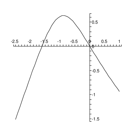
Figure 1: Typical behaviour of $Y$ as a function of $\eta$ for de Sitter solutions ($\epsilon=+1$). The function interpolates between two asymptotically linear regimes. The gradient is always positive as $\eta\rightarrow-\infty$ and negative as $\eta\rightarrow+\infty$.

Figure 2: Typical behaviour of $Z$ as a function of $\eta$ for de Sitter solutions ($\epsilon=+1$). The solutions are asymptotically linear with different gradients. For a suitable choice of initial data the gradient can change sign as in Fig. 2.

The solutions of ref. GGP discussed above satisfy these condition in the special case where $\lambda_{3}^{\pm}=\pm|\lambda_{3}|$, and in this case we know the 4D geometries are flat. In general, however, both the parameters $\lambda_{3}^{\pm}$ are not determined by the one constant $\lambda_{3}$, and so in the general case the sum $\sum_{\pm}f_{\pm}$ does not vanish, leading (c.f. eq. (9)) to the conclusion that the corresponding 4D geometries cannot be flat. We have been unable to obtain analytic solutions to these equations, but there is no obstruction to their integration. They can be solved numerically leading to numerical profiles such as those given in figures (2) and (2).

V Discussion

In this paper our focus has been on solutions to the field equations of the coupled dilaton/$p$-form/Einstein equations of some $D$-dimensional supergravities, for which $n$ of the dimensions are maximally symmetric. Such solutions could arise, for instance, in compactifications from $D$ to $n$ dimensions within a Kaluza-Klein scenario.

Our main result in this paper is to provide a fairly general relation between the curvature of the maximally symmetric $n$ dimensions in terms of the (potentially singular) asymptotic behaviour of the various fields in the vicinity of any brane sources which may be situated about the internal $d=D-n$ dimensions. This relationship allows an explicit connection to be made between this curvature and the properties of the branes which source the geometry. It is only once this connection is made explicit that it becomes possible to address whether the existence of flat solutions requires a technically unnatural fine-tuning of brane properties.

In particular, we use this connection in chiral 6D gauged supergravity to show the existence of compactifications to 4D de Sitter and anti-de Sitter geometries having arbitrary curvature. Since the curvature can be arbitrary it can in particular be small, implying that these new solutions can be obtained by small perturbations from the previously-known flat solutions. Since many of the flat solutions, such as those described by the rugby ball of ref. sled , are known to have positive tensions it follows that at least some of these new solutions can also be sourced by branes having physically reasonable properties.

The existence of such solutions certainly complicates a self-tuning solution of the cosmological constant problem along the lines of Ref. sled in several ways because it shows that maximal symmetry in 4 dimensions is insufficient to guarantee these dimensions must be flat. This means that there are now two ways in which perturbations on a brane might destabilize a flat solution: either by starting a time-dependent runaway or by generating a maximally-symmetric but curved 4 dimensions. The key issue which remains is whether the choices of brane properties which exclude these two options are stable under renormalization. The results of this paper provide the prerequisite for answering this issue, because they show that the magnitude of the effective cosmological constant problem is determined by the asymptotic form of the bulk fields, which are in turn fixed by the properties of the brane action which we renormalize.

For instance, let us suppose that the branes do not couple to the dilaton, so that $\lambda=0$ in equation (21), and suppose that this condition were preserved under quantum corrections (something which must be explicitly checked). In this case we anticipate that the boundary condition for the dilaton near each brane should be $\varphi^{\prime}=0$, and so $q_{\pm}=0$. However in such a case the 6D Kasner conditions demand that the only allowed solutions are those describing conical branes, and for these our sum-rule implies the only maximally symmetric solution is Minkowski. Thus if we start out in one of the conical GGP solutions and perturbation (like renormalization or a phase transition on one brane) changes the effective brane tension without growing a dilaton coupling, then the de Sitter and anti-de Sitter minima discovered here cannot be reached. Furthermore the system cannot evolve to one of the other non-conical GGP solutions unless some nontrivial dilaton coupling develops. In such a case it is likely that the system evolves towards an as-yet-undiscovered time-dependent runaway solution. If so, the central question would become how fast the runaway is, and can it successfully describe the observed Dark Energy? We intend to return to these questions in a subsequent publication.