A novel braneworld model with a bulk scalar field

Abstract

We consider a new braneworld model with a bulk scalar field coupled to gravity. The bulk scalar action is inspired by the proposed low energy effective action around the tachyon vacuum. A class of warped geometries representing solutions of this Einstein-scalar system for a specific scalar potential is found. The geometry is non singular with a decaying warp factor and a negative Ricci curvature. The solution of the hierarchy problem is obtained using this type of warping. Though qualitatively similar to the usual Randall–Sundrum I model there are interesting quantitative differences. Additionally, in the RS-II set up the graviton zero mode as well as spin half massless fermions are found to be localised on the brane.

I Introduction

The study of extra dimensions (D $>$ 4) has been of considerable interest to theoretical physicists ever since Kaluza-Klein introduced them in their attempt to unify gravity with electromagnetism kk . Over the last few decades, the notion of extra dimensions has been discussed with renewed enthusiasm in the context of string theory string where their presence is inevitable. More recently, attention has shifted toward the braneworld picture - in which our four dimensional universe (3-brane) is viewed as an embedded hypersurface in a higher dimensional bulk spacetime. In the now-popular Randall-Sundrum models (known as RS I and RS II) rs of warped (nonfactorisable) spacetimes the extra dimensions exist, can be compact or non-compact, but the usual schemes of compactification are replaced by the notion of localisation of fields on the brane. The RS-I model provides us with a solution of the gauge hierarchy problem whereas RS-II shows us how the higher dimensional gravity can still reproduce Newtonian gravity on the brane. Several problems exist with the RS models, some of which have been tackled by introducing appropriate modifications modrs .

In the RS models, the bulk is essentially vacuum but with a negative (five dimensional) cosmological constant (AdS spacetime). This leads to a problem of stability of the branes – a matter of concern in the two–brane (RS I) scenario. To remedy this, bulk fields are introduced, in particular, a scalar field with a potential radion . A bulk scalar also provides us with a way of generating the braneworld as a domain wall in five dimensions–these are the so–called thick branes. The last few years has seen much work being carried out on diverse aspects of such braneworld models with variety of bulk field configurations rs ; thick . In the context of such newer models with bulk fields, issues such as localisation of various types of matter fields loc ; gravloc ; fermiloc , cosmological consequences cosmo and particle phenomenology in the braneworld context particle have been addressed to some extent. Further consequences of new types of bulk matter and their resulting effects still remains an open arena of research.

Recently there has been a lot of activity on a newly proposed scalar field theory - namely ‘tachyon matter’ arising in the context of string theory sen . Briefly, one can say that open string tachyons (attached to D–branes and reflecting D–brane instability), residing on the unstable (tachyonic) maximum of the tachyon potential can acquire a vacuum expectation value (condensate) and roll down to a stable configuration. The energy of such a tachyon condensate has been calculated in string field theory. The effective action thus obtained is somewhat uncommon due to its special form. It is completely different from the usual scalar field action and resembles, in some sense, a Born–Infeld type action bi . Though proposed by several authors independently tachyon its physical consequences have been analysed in greater detail recently by Sen sen . It has been shown that such a scalar field might play a role in cosmology in the context of dark matter/energy. This is because the effective energy–momentum tensor can be shown to be equivalent to that of noninteracting, nonrotating dust tachycosmo . Since, currently, there is no unique, experimentally verifiable choice for bulk matter, it is surely useful to explore various possibilities newbulk . This has motivated us to consider the tachyon condensate as a bulk field coupled to gravity and study its effects on the geometry. It is worth mentioning here that one might also visualise the tachyon condensate action as a new type of scalar field action without making any particular reference to string theory as such. The dynamics of this scalar field, both classical and quantum is of interest in its own right and has been investigated from this standpoint too.

The bulk geometry is taken to be non-factorisable (warped). We first obtain an exact solution of the full set of Einstein-scalar equations with a given scalar potential. Thereafter, we address the hierarchy problem in a RSI set-up. In the subsequent section, we analyse the graviton zero mode and demonstrate its localisation in RSII set-up. Finally, we concentrate on fermion (massless) localisation and conclude with a summary of the results obtained.

II The model and the exact solution

Let us begin with the action for the bulk scalar field sen given by

$$S_{T}=\alpha_{T}\int d^{5}x\sqrt{-g}V(T)\sqrt{1+g^{MN}\partial_{M}T\partial_{N}T}$$ (1)

where $\alpha_{T}$ is an arbitrary constant, $g_{MN}$ being the five dimensional metric. The scalar field is represented by T and V(T) corresponds to its potential. The constant $\alpha_{T}$ can take either positive or negative values. The energy momentum tensor corresponding to the above action is given by :

$$T_{MN}^{(T)}=\frac{\alpha_{T}}{2}\left[g_{MN}V(T)\sqrt{1+(\nabla T)^{2}}-\frac{V(T)}{\sqrt{1+(\nabla T)^{2}}}\partial_{M}T\partial_{N}T\right]$$ (2)

For an appropriate choice of $\alpha_{T}$ and V(T) it is possible to keep the geometry, produced by the above action along with gravity, unaltered with respect to the signature change of $\alpha_{T}$. Note the unusual form of the action - the potential is multiplied with a square root function containing the metric and derivatives of the scalar field. This inherent novelty of the action has generated a lot of activity. The full five dimensional action will also contain an Einstein–Hilbert term along with the contributions from the brane vacuum energies.

The action of the model is

$$S = S_{G}+S_{T}+S_{B}$$ (3)

$$S_{G} = 2M^{3}\int\sqrt{-g}Rd^{5}x$$ (4)

$$S_{B} = -\int\sum_{j}\tau_{(j)}\sqrt{-\tilde{g}^{(j)}}d^{4}x$$ (5)

where $\tilde{g}_{\mu\nu}^{(j)}$ is the induced metric on the brane and $\tau_{(j)}$ is the vacuum energy density of the brane located at $\sigma=\sigma_{j}$. There are two branes in RSI set-up and a single brane in RSII set-up. Variation of the total action w.r.t. $g_{MN}$ leads to the Einstein–scalar equation and that w.r.t. T gives rise to the scalar field equation.

We assume a line element, in the five dimensional bulk, of the form:

$$ds^{2}=e^{-2f(\sigma)}(\eta_{\mu\nu}dx^{\mu}dx^{\nu})+d\sigma^{2}$$ (6)

The warp factor f($\sigma$) and the scalar field T are considered to be function of $\sigma$ only. With these ansatz, the Einstein-scalar equation reduces to the following system of coupled, nonlinear ordinary differential equations :

$${f^{\prime}}^{2} = \frac{a}{2}\frac{V(T)}{\sqrt{1+T^{\prime 2}}}$$ (7)

$$f^{\prime\prime} = -aV(T)\frac{T^{\prime 2}}{\sqrt{1+T^{\prime 2}}}+\frac{1}{12M^{3}}\sum_{j}\tau_{j}\delta(\sigma-\sigma_{j})$$ (8)

where $a=\frac{\alpha_{T}}{12M^{3}}$ and prime denotes derivative with respect to the coordinate $\sigma$. We have been able to find an exact analytical solution of the above set of equations (2.7) - (2.8) for the scalar field potential

$$V(T)=\frac{8}{ak^{2}}\frac{1}{T^{4}}\left(1+\frac{k^{2}}{4}T^{2}\right)^{\frac{1}{2}}$$ (9)

where $k$ is an arbitrary constant. It is straightforward to show that the potential remains non-singular as long as the scalar field does not become zero. We will show that in our set of exact solutions the scalar field T, never becomes zero for any finite value of the extra coordinate. It is worth noting that our solution is for $\alpha_{T}>0$. If we were to take $\alpha_{T}<0$ (which is the usual choice, $\alpha_{T}=-1$ in the literature on tachyon matter) the same solution will be valid provided we invert the potential by absorbing the minus sign in the definition of $V(T)$. Note that with $a\rightarrow-a$ and $V(T)\rightarrow-V(T)$ the field equations remain unchanged.

Figure 1: The scalar field potential is depicted in the above figure for the parameters $a_{1}=k=1$ and $\alpha_{T}$ having unit positive value

The explicit forms of the warp factor and the scalar field are given by :

$$f(\sigma)=-\frac{a_{1}}{k}e^{-k|\sigma|}$$ (10)

$$T(\sigma)=\sqrt{\frac{2}{ka_{1}}}e^{\frac{k}{2}|\sigma|}$$ (11)

for the entire domain of the extra dimension, $-\infty<\sigma<\infty$. Where $a_{1}$ is an arbitrary constant and $k$ is a scale of the order of Planck scale. It is important to note that the metric warp factor is a super exponential function which decays as one moves along the transverse dimension. The scalar is an exponentially growing function of $\sigma$. Also, the scalar field never becomes zero, keeping the potential always non-singular.

Figure 2: The warp factor is a decaying function of the higher dimensional coordinate $\sigma$. We have used the same set of parameters as in the previous figure

The line element in this warped spacetime is given by

$$ds^{2}=e^{\frac{2a_{1}}{k}e^{-k|\sigma|}}(\eta_{\mu\nu}dx^{\mu}dx^{\nu})+d\sigma^{2}$$ (12)

The Ricci scalar, R, for this background metric in the regions $\sigma\neq\sigma_{j}$ turns out to be :

$$R = -\left(8a_{1}k+20a_{1}^{2}e^{-k|\sigma|}\right)e^{-k|\sigma|}$$ (13)

Notice that R is always negative and approaches zero for $\sigma\rightarrow\pm\infty$. This implies that the spacetime is asymptotically flat.

It will be interesting to know the matter stress energy that gives rise to such a bulk line element. The energy density and pressures (for $\sigma\neq\sigma_{j}$) are given as

$$\rho = -p_{i}=-(6{a_{1}}^{2}e^{-k|\sigma|}+3a_{1}k)e^{-k|\sigma|}$$ (14)

$$p_{\sigma} = 6a_{1}^{2}e^{-2k|\sigma|}$$ (15)

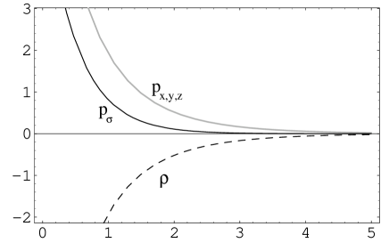
Figure 3: The matter stress energy in the region $\sigma\neq\sigma_{j}$ and $\sigma>0$ is plotted with same set of parameters

for the range of extra dimensional coordinate excluding the location of the brane(s). In Fig. (3) we have plotted the pressures and energy density as a function of the transverse coordinate $\sigma$ (for $\sigma\neq\sigma_{j}$ and $\sigma>0$). For $\sigma<0$ the pressures and energy density are the same because the functions are even in nature.

It is worth mentioning that the matter stress-energy which acts as a source for the warped geometry satisfies the SEC ($\rho+\sum p_{j}\geq 0$) though the WEC ($\rho\geq 0$) and NEC ($\rho+p_{j}\geq 0$) are violated ec .

III RS I two–brane model and the hierarchy problem

In RS I there are two branes located at $\sigma=0$ and $\sigma=\pi r_{c}$. The extra dimension between the two 3–branes is defined on a $S_{1}/Z_{2}$ orbifold with branes located at the orbifold fixed points $\sigma=0,\pi r_{c}$. Let us now focus on the equation (2.8) which reduces to the following form in the RSI set-up.

$$3f^{\prime\prime}=-\frac{1}{4M^{3}}\frac{\alpha_{T}V(T)T^{\prime 2}}{\sqrt{1+T^{\prime 2}}}+\frac{\tau_{(1)}}{4M^{3}}\delta(\sigma)+\frac{\tau_{(2)}}{4M^{3}}\delta(\sigma-\pi r_{c})$$ (16)

where, M is the fundamental scale in five dimensions. The second derivatives of the warp factor $f(\sigma)=-\frac{a_{1}}{k}e^{-k|\sigma|}$ (assuming periodicity of $f(\sigma)$) is given by :

$$f^{\prime\prime}(\sigma) = -a_{1}ke^{-k|\sigma|}+2a_{1}e^{-k|\sigma|}\left[\delta(\sigma)-\delta(\sigma-\pi r_{c})\right]$$ (17)

We assume that the bulk scalar field does not have any interaction with on–brane matter. Comparing Eqn. (3.1) with Eqn. (3.2) we obtain the tension on the two branes as

$$\tau_{(1)} = 24M^{3}a_{1}$$ (18)

$$\tau_{(2)} = -24M^{3}a_{1}e^{-k\pi r_{c}}$$ (19)

It can be seen from the above relations that unlike the RS I case the brane tensions are not equal in magnitude. There is a scaling in the tension of the brane at $\sigma=\pi r_{c}$ which we consider as the visible brane. The visible brane is a negative tension brane and its tension can be chosen to be lower than that of the positive tension brane.

In order to address the hierarchy problem we integrate the bulk gravity action over the extra dimension and compare it with the usual Einstein–Hilbert action for four dimensional gravity. This results in the following relation between the four dimensional Planck scale ($M_{Pl}$) and the fundamental five dimensional scale (M) :

$$M_{Pl}^{2}=\frac{2M^{3}}{k}\left[Ei\left(\frac{2a_{1}}{k}\right)-Ei\left(\frac{2a_{1}}{k}e^{-k\pi r_{c}}\right)\right]$$ (20)

where, “Ei” represents the exponential integral function ei . For $\frac{a_{1}}{k}=39$ we obtain a solution of the hierarchy problem for $kr_{c}=5$. For such typical values one finds that a choice of fundamental (higher dimensional) scales of the TeV range for all parameters (such as five dimensional Planck scale, $m_{0}$ etc.) would reproduce the four dimensional Planck scale of $10^{19}$ GeV (using the relation in Eqn 3.5) leaving the masses on the visible brane in the TeV range. This shows that the heirarchy of scales is a ‘derived’ notion and there is no heirarchy of scales in a higher dimensional world. Note the reduction of the value of $kr_{c}$ as compared to the RS I case. This is essentially due to the modified nature of the warp factor in our solution here. Following RS I, we can also show how the Higgs vacuum expectation value and the masses of elementary particles will scale on the negative tension brane ($m=m_{0}e^{e^{-kr_{c}\pi}}$).

IV RS II one–brane Model and localisation of fields

In order to investigate whether the metric tensor fluctuations give consistent four dimensional gravity we consider the RS-II set up i.e. the transverse space is now infinitely extended rs . The regulator brane is now sent to infinity by making the radius of the extra dimension to be infinite. The positive tension brane is now treated as our visible world. Let us consider a general linearized tensor fluctuation to the metric and check the behavior of gravitational zero modes.

IV.1 Gravity localisation

We restrict ourselves for the metric fluctuation, $h_{\mu\nu}(x^{\mu},\sigma)$ of the 4-dimensional world on the three brane and consider the following metric :

$$ds^{2}=e^{-2f(\sigma)}(\eta_{\mu\nu}+h_{\mu\nu}(x^{\mu},\sigma))dx^{\mu}dx^{\nu}+d\sigma^{2}$$ (21)

Keeping the background in the non-conformally flat form we proceed to analyse the gravitational fluctuation under RS gauge conditions - (i) $\partial_{\mu}h^{\mu}_{\nu}=0$, (ii) $h^{\mu}_{\mu}=0$. The linearized gravity fluctuation equation is then simply the covariant scalar wave-equation. For a fluctuation of the form $h_{\mu\nu}(x^{\mu},\sigma)=\phi(\sigma)\bar{h}_{\mu\nu}(x^{\mu})$ with $\nabla^{\rho}\nabla_{\rho}{\bar{h}_{\mu\nu}}=m^{2}\bar{h}_{\mu\nu}$ , m being the four dimensional mass of Kaluza-Klein mode we perform the mode analysis thick ; gravloc . The equation satisfied by $\phi(\sigma)$ always admits a zero mode (i.e. m = 0) solution, $\phi_{0}(\sigma)=constant$. Now, inserting this solution to the action gravloc from which the gravity fluctuation equation is derived one obtains the following normalisability condition for the zero-mode wave function

$$\int{e^{-2f(\sigma)}d\sigma}<\infty$$ (22)

Using the expression of $f(\sigma)$ obtained in equation (2.9) we find that the integrand is finite over the entire domain of the extra dimension, from which we conclude that the above condition is satisfied in our case. Therefore it can be said that gravity is localised around the brane with the zero mode being the massless graviton.

IV.2 Fermion Localisation

We now turn our attention to the localization of spinor fields on the brane. The bulk fermion coupled to the scalar field in 5D gives rise to two chiral fermionic zero modes in four dimensions. Depending on the nature of the coupling one of these two modes is found to be localized on the brane while the other is not loc ; fermiloc . In the background of the scalar field coupled to gravity we find that the left chiral modes only can be confined to the brane for a positive Yukawa coupling.

The Lagrangian for a Dirac fermion propagating in the five dimensional warped space with the metric (2.5) is :

$$\sqrt{-g}{\cal{L}}_{Dirac}=\sqrt{-g}\hskip 2.168pt(i\bar{\Psi}\Gamma^{M}{\cal{D}}_{M}\Psi-\eta_{F}\bar{\Psi}\mbox{F}(T)\Psi)$$ (23)

The matrices $\Gamma^{a}=(e^{f(\sigma)}\gamma^{\mu},-i\gamma^{5})$ provide a four dimensional representation of the Dirac matrices in five dimensional curved space. Where $\gamma^{\mu}$ and $\gamma^{5}$ are the usual four dimensional Dirac matrices in chiral representation.

The Dirac Lagrangian in 5D curved spacetime then reduces to the following form

$$\sqrt{-g}{\cal{L}}_{Dirac}=e^{-4f(\sigma)}\bar{\Psi}\left[ie^{f(\sigma)}\gamma^{\mu}\partial_{\mu}+\gamma^{5}(\partial_{4}-2f^{\prime}(\sigma))-\eta_{F}\mbox{F}(T)\right]\Psi$$ (24)

The dimensional reduction from 5D to 4D is performed in such a way that the standard four dimensional chiral particle theory is recovered. Separating the variables the five dimensional spinor can be written as: $\Psi(x^{\mu},\sigma)=\Psi(x^{\mu})\xi(\sigma)$. Since the four dimensional massive fermions require both the left and right chiralities it is convenient to organise the spinors with respect to $\Psi_{L}$ and $\Psi_{R}$ which represent four component spinors living in five dimensions given by $\Psi_{L,R}=\frac{1}{2}(1\mp\gamma_{5})\Psi$. Hence the full 5D spinor can be split up in the following way

$$\Psi(x^{\mu},\sigma)=\left(\Psi_{L}(x^{\mu})\xi_{L}(\sigma)+\Psi_{R}(x^{\mu})\xi_{R}(\sigma)\right)$$ (25)

where $\xi_{L.R}(\sigma)$ satisfy the following eigenvalue equations

$$e^{-f(\sigma)}\left[\partial_{\sigma}-2f^{\prime}(\sigma)-\eta_{F}\mbox{F}(T)\right]\xi_{R}(\sigma) = -m\xi_{L}(\sigma)$$ (26)

$$e^{-f(\sigma)}\left[\partial_{\sigma}-2f^{\prime}(\sigma)+\eta_{F}\mbox{F}(T)\right]\xi_{L}(\sigma) = m\xi_{R}(\sigma)$$ (27)

Here $m$ denotes the mass of the four dimensional fermions. The full 5D action reduces to the standard four dimensional action for the massive chiral fermions, when integrated over the extra dimension fermiloc , if (a) the above equations are satisfied by the bulk fermions and (b) the following orthonormality conditions are obeyed.

$$\int_{-\infty}^{\infty}e^{-3f(\sigma)}\xi_{L_{m}}\xi_{L_{n}}d\sigma=\int_{-\infty}^{\infty}e^{-3f(\sigma)}\xi_{R_{m}}\xi_{R_{n}}d\sigma=\delta_{mn}$$ (28)

$$\int_{-\infty}^{\infty}e^{-3f(\sigma)}\xi_{L_{m}}\xi_{R_{n}}d\sigma=0$$ (29)

The massless (i.e. $m=0$) fermions for a Yukawa coupling of the form $F(T)=T$ are represented by the following wave functions

$$\xi_{L}=exp\left[\frac{2}{k}\left(-a_{1}e^{-k|\sigma|}-\eta_{F}\sqrt{\frac{2}{a_{1}k}}e^{\frac{k}{2}|\sigma|}\right)\right]$$ (30)

$$\xi_{R}=exp\left[\frac{2}{k}\left(-a_{1}e^{-k|\sigma|}+\eta_{F}\sqrt{\frac{2}{a_{1}k}}e^{\frac{k}{2}|\sigma|}\right)\right]$$ (31)

If the coupling constant, $\eta_{F}=0$, it is clear from the above expressions that both the left and right chiral modes decay away from the brane. If $\eta_{F}>0$ then $\xi_{L}$ decays but $\xi_{R}$ grows and the reverse phenomena takes place for $\eta_{F}<0$.

Figure 4: The left chiral zero modes are localised around the brane. We have used unit coupling constant and kept the set of parameters unchanged

In Fig.(4) we have shown the nature of variation of the left chiral mode w.r.t. the extra dimension. The left chiral mode is localised around the brane for positive Yukawa coupling whereas for an opposite Yukawa coupling we get the right chiral modes to be confined around the brane.

V Conclusion

We now summarize below the results obtained.

(i) We have considered the tachyon condensate as a bulk scalar coupled to gravity. Exact analytical expressions for the warp factor and scalar field have been obtained from the solution of the full Einstein-scalar equations. The nature of the scalar field potential depends on the sign of the coupling constant $\alpha_{T}$. The background geometry obtained in this case is however described by a negative, non-constant Ricci scalar with delta function singularity at the location of the brane; it goes to zero asymptotically. The stress-energy tensor, giving rise to this geometry, violates the null and weak energy conditions whereas it satisfies the strong energy condition.

(ii) The resolution of the gauge hierarchy problem is attempted in this background geometry for a RS I type model consisting of two branes situated at the two fixed points in an $S^{1}/Z_{2}$ orbifold. We find that the brane tensions are of unequal and opposite magnitude. The relation between the five dimensional fundamental mass scale and the four dimensional Planck scale can be brought to same order for a particular choice of the model parameters. We also point out how the Higgs expectation value and the masses scale on the negative tension brane.

(iii) The graviton zero mode in this background geometry is found to localised and normalisable. Additionally, fermionic zero modes with left chirality are found to be localised around the brane in the presence of a Yukawa coupling between the scalar and spinor field. The right chiral modes may be found on the brane for an opposite value of the Yukawa coupling parameter.

The fate of the massive graviton and fermion modes in this background geometry is an obvious next question we need to answer. Furthermore, we also would like to know about cosmological solutions on the brane by assuming a flat FRW on–brane line element. We hope to come back with these issues and other related ones in future.

References

- (1) T. Kaluza, Sitzungsber. Preuss. Akad. Wiss., Phys-Math.Kl., Berlin Math. Phys., Bd. K1 966 (1921) ; O. Klein, Z. Phys. 37, 895 (1926); A. Salam and J. Strathdee, Ann. Phys. 141, 316 (1982); M. J. Duff, B.E.W. Nilsson and C. N. Pope, Phys. Rep. 130 C, 1 (1986); T. Appelquist, A. Chodos and P. G. O. Freund, Modern Kaluza–Klein Theories, Reading, MA, Addison–Wesley (1987).
- (2) M. S. Green, J. H. Schwarz and E. Witten, Superstring theory, Cambridge University Press (1987); J. Polchinsky, String theory, Cambridge University Press (1997);
- (3) L. Randall and R. Sundrum, Phys. Rev. Lett. 83, 3370 (1999); ibid Phys. Rev. Lett. 83, 4690 (1999)
- (4) W. D. Goldberger and M. B. Wise, Phys. Rev. Lett. 83, 4922 (1999); R. Gregory, V. A. Rubakov and S. M. Sibiryakov, Phys. Rev. Lett. 84, 5928 (2000); G. Dvali, G. Gabadadze and M. Porrati, Phys. Lett. B484, 112, (2000)
- (5) P. J. Steinhardt, Phys. Lett. B 462 41, (1999); C. Csaki, M. Graessser, L. Randall nad J. Terning, Phys. Rev. D 62 045015 (2000); C. Charmousis, R. Gregory and V. A. Rubakov, Phys. Rev. D 62 067505 (2000); P. Brax, C. Bruck and A. C. Davis and C. S. Rhodes, Phys. lett. B 531 , 135, (2002)
- (6) C. Csaki, J. Erlich, C. Grojean and T. Hollowood, Nucl. Phys. B 584, 359 (2000) ; O. DeWolfe, D. Z. Friedman. S. S. Gubser and A. Karch, Phys. Rev. D 62 046008 (2000); C. Csaki, J. Erlich, T. Hollowood and Y. Shirman, Nucl. Phys. B 581, 309 (2000) H. Davoudiasl, J.L. Hewett and T.G. Rizzo, Phys.Lett. B 473 43 (2000); S. C. Davis, JHEP 0203, 054 (2002); E. E. Flanagan, S.H. Henry Tye and I. Wasserman, Phys.Lett. B 522 155 (2001);
- (7) B. Bajc and G. Gabadadze, Phys. Lett. B 474, 282 (2000);
- (8) J. Garriga and T. Tanaka, Phys. Rev. Lett. 84 2778 (2000); J. Lykken and L. Randall, JHEP 0006, 014, (2000); A. Karch and L.Randall, JHEP 0105, 017, (2001); S. B. Giddings, E. Katz and L. Randall, JHEP 0003 (2000); I. Brevik, K. Ghoroku, S. D. Odintsov and M. Yahiro, Phys.Rev. D66, 064016 (2002)
- (9) S. L. Dubovsky, V. A. Rubakov and P. G. Tinyakov, Phys. Rev. D 62, 105011 (2000) R. Jackiw and C. Rebbi, Phys. Rev. D 13, 3398 (1976); Y. Grossman and N. Neubert, Phys. Lett. B 474 361 (2000) R. Jackiw and C. Rebbi, Phys. Rev. D 13, 3398 (1976); Y. Grossman and N. Neubert, Phys. Lett. B 474 361 (2000); C. Ringeval, P. Peter, J. P. Uzan, Phys. Rev. D 65, 044416 (2002); S. Ichinose, Phys.Rev. D 66, 104015 (2002)
- (10) D. Langlois, gr-qc/0102007 (Proceedings of the 9th Marcel Grossmann meeting, July 2000 (Rome); gr-qc/0205004 (Proceedings of Journees Relativistes, Dublin 2001 and references therein ; E. Flanagan, S.H. Henry Tye and I. Wasserman, Phys. Rev. D 62, 024011 (2000); H. Stoica, S. H. Henry Tye and I. Wasserman, Phys. Letts. B 482, 205 (2000); J. S. Alcaniz, Phys. Rev. D65, 123514, (2002)
- (11) M. Besancon, hep-ph/0106165 ; Y. A. Kubyshin, hep-ph/0111027 and references therein.
- (12) A. Sen, JHEP 0204, 048, (2002); ibid JHEP 0207, 065 (2002); ibid Mod. Phys. Letts. A 17, 1797 (2002);
- (13) G. W. Gibbons, K. Hori and P. Yi, Nucl. Phys. B 596 (2001) 136; A. Sen, J. Math. Phys 42 (2001) 2844.
- (14) M. R. Garousi, Nucl. Phys. B 584, 284 (2000); J. Kluson, Phys Rev. D 62; E. A. Bergshoeff, M. de Roo, T. C. de Witt, E. Eyreas and S. Panda, JHEP 0005, 009 (2000);
- (15) G.W. Gibbons, Phys Letts. B 537, 1 (2002); M. Fairbairn and M. H. G. Tytgat, Phys. Lett. B 546, 1, (2002); G. Shiu and I. Wasserman, Phy. Lett. B 541, 6, (2002)
- (16) B. Mukhopadhyaya, S. Sen, S. SenGupta, Phys.Rev. D 65 124021 (2002); M. Gogberashvili, Phys.Lett. B 553, 284 (2003); R. Koley and S. Kar, Mod. Phys. Letts. A 20, 363 (2005) ; K. Ghoroku, hep-th/0402102;
- (17) For a useful summary on the details of the energy conditions see Lorentzian Wormholes : from Einstein to Hawking by Matt Visser (AIP, 1995)
- (18) M. Abrmowitz and C. A. Stegan, Handbook of Mathematical Functions with Formulas, Graph, and Mathematical Tables (Dover, New York, 1972)