Accelerating cosmologies from exponential potentials

Abstract:

An exponential potential of the form $V\sim\exp(-2c\,\varphi/M_{p})$ arising from the hyperbolic or flux compactification of higher-dimensional theories is of interest for getting short periods of accelerated cosmological expansions. Using a similar potential but derived for the combined case of hyperbolic-flux compactification, we study the four-dimensional flat (and open) FLRW cosmologies and give analytic (and numerical) solutions with exponential behavior of scale factors. We show that, for the M-theory motivated potentials, the cosmic acceleration of the universe can be eternal if the spatial curvature of the 4d spacetime is negative, while the acceleration is only transient for a spatially flat universe. We also briefly comment on the size of the internal space and its associated geometric bounds on massive Kaluza-Klein excitations.

1 Introduction

A tentative acceptance of cosmic acceleration of the universe [1] has stimulated many works on string or M theory cosmology [2, 3, 4, 5, 6, 8, 9, 10, 7, 11, 12, 13, 14]. Though it is not explored yet whether string or M-theory predicts the distinctive features of our universe, like a spatially flat (or open) four dimensional expanding universe with small matter fluctuations, most physicists would believe that a four dimensional cosmology should be derived from a fundamental theory of gravity and particle interactions. This fundamental theory could be a theory of supergravity or superstring origin, or even a theory without the need of extra dimensions or supersymmetry (e.g. loop quantum gravity). Nonetheless, it is quite interesting that cosmic acceleration can arise from compactifications of higher-dimensional theories on hyperbolic spaces without or with fluxes [3, 4, 5, 6, 7]. These solutions, along with their many generalizations  [8, 9, 10, 7, 11, 12, 13] deal with time-dependent scale factors of internal spaces, thereby overcoming a difficulty of “no-go theorem” given for a de Sitter type compactification in supergravity theories with static (and warped) extra dimensions [15].

When studying the dynamics of the inflationary universe, in a four-dimensional effective theory, one considers the Lagrangian density

$${\cal L}=\sqrt{-g}\,\left(\frac{M_{P}^{2}}{2}\,{\cal R}[g]-(\partial\varphi)^{2}-2V(\varphi)\right)\,$$ (1)

with canonically normalized kinetic and potential terms. Of particular importance is the choice of the potential $V(\varphi)$ whose form depends on particle physics or compactifications used to derive a lower dimensional effective field theory. One would like to derive potentials that allow inflation in the early universe and/or acceleration in the current cosmological epoch. Both cases may be explained in a typical manner by postulating some suitable scalar potentials.

Recently some progress has been made about inflation within string theory [16] by keeping the system in the string theory de Sitter vacuum  and by constructing a scalar potential in the $D3/\bar{D}3$ warped brane background [18]. These mathematical frameworks assume that the metric of a compact non-singular internal $m$-manifold $\Sigma_{m}$ is time-independent, and in turn, inflation is non-generic which involves some degree of functional fine tuning. In this paper we consider scalar fields in cosmology by allowing the metric on $\Sigma_{m}$ to be time-dependent.

For many classical compactifications of effective supergravity theories, the scalar potentials are of the form $V\sim\exp(-2c\,\varphi/M_{P})$ with the (dilaton) coupling constant $c\sim{\cal O}(1)$. The cosmological models with such a potential have been known lead to interesting physics in a variety of context, ranging from existence of accelerated expansions [19] to cosmological scaling solutions [20], see also, e.g., [21, 22] for some related discussions. It is also worth noting that an attractor solution with a simple exponential potential of the above form may lead to cosmic acceleration for natural values of model parameters [23].

A number of authors have studied the effects of exponential potentials on M-theory cosmology, including the recent papers concerning hyperbolic or flux compactification and accelerated expansion. So far no general discussion has been given for the combined effects of hyperbolic-flux compactification, see, however, Refs. [6, 11] for some qualitative arguments. In addition, most authors have studied only a spatially flat universe, and this in turn leads to the observation that the accelerated period in these models is typically preceded by a period when the universe was dominated by the kinetic energy of the scalar field. So in this note we allow the spatial curvature ($k$) of the 4d spacetime to take the value $k=0$ or $k=\pm 1$. We show that the accelerated expansion of our universe may continue forever if $k=-1$. This possibility was pointed out in [7, 19]; here we make the earlier discussions more precise with further analysis and new results, taking into account the combined effects of hyperbolic extra dimensions and background fluxes.

2 Compactification with fluxes

Let us consider that the M theory spacetime is the product of a four dimensional spacetime ${M}_{4}$ and an internal compact space $\Sigma_{m,k_{1}}$, namely,

$$ds_{4+m}^{2}={\rm e}^{-m\phi(\xi)}\,g_{\mu\nu}(x)dx^{\mu}dx^{\nu}+r_{c}^{2}\,{\rm e}^{2\phi(\xi)}\,d\Sigma^{2}_{m,k_{1}}$$ (2)

with $\tilde{R}_{ab}(\Sigma_{m,k_{1}})=k_{1}(m-1)\tilde{g}_{ab}\,r_{c}^{-2}$, where $r_{c}$ is the radius of curvature of internal space ($a,b$ go over the dimensions of the internal space). In suitable coordinates, $k_{1}=-1,\,0,$ or $+1$, respectively, for hyperbolic, flat or spherical manifold . Since the metric (2) is written in Einstein conformal frame, the effective 4d Planck mass $M_{P}$ does not depend on time scale but (only) on a spatial volume of the highly curved internal manifold, the latter scales as $\sim r_{c}^{m}\,e^{\alpha}$, where $\alpha$ depends on the topology of the internal manifold [24].

Together with the four-form field strength ${}_{*}F_{[4]}=2b\,\mbox{Vol}(\Sigma_{m,k_{1}})$, $b$ being the field strength parameter, upon the dimensional reduction we get [6, 13]

$$I={M_{P}^{2}}\int d^{4}x\left(\frac{{\cal R}[g]}{2}-\frac{m(m+2)}{4}\left(\partial\phi\right)^{2}-b^{2}{\rm e}^{-3m\phi}+k_{1}\,\frac{m(m-1)}{2\,r_{c}^{2}}\,{\rm e}^{-\,(m+2)\phi}\right),$$ (3)

where $M_{P}^{-1}=\sqrt{8\pi G}\equiv\kappa$ is the reduced Planck mass. The solution following from $(4+m)$ dimensional field equations is

$$ds_{4+m}^{2}={\rm e}^{-m\phi(\xi)}\left(-\,S^{6}\,d\xi^{2}+S^{2}\,d\vec{x}_{3,k}^{2}\right)+r_{c}^{2}\,{\rm e}^{2\phi(\xi)}\,d\Sigma^{2}_{m,k_{1}},$$ (4)

$$\phi(\xi)=\frac{\ln(A\,B)}{m-1},\quad S^{2}={[A]}^{{m}/{m-1}}\,{[B]}^{(m+2)/3(m-1)},$$ (5)

$$A(\xi)=\left\{\begin{array}[]{l}\frac{r_{c}}{(m-1)}\,\frac{\lambda\,\beta}{\sinh\left[\lambda\beta\,|\xi|\,\right]},\quad~{}~{}k_{1}=-1,\\ {\rm e}^{\lambda\beta\,\xi},\quad~{}~{}~{}~{}~{}~{}~{}~{}~{}~{}~{}~{}~{}~{}~{}k_{1}=0,\\ \frac{r_{c}}{(m-1)}\,\frac{\lambda\,\beta}{\cosh\left[\lambda\beta\,\xi\,\right]},\quad~{}~{}~{}k_{1}=+1,\end{array}\right.\$$ (9)

$$B(\xi)=\left\{\begin{array}[]{l}{\rm e}^{-3\lambda\,\xi},~{}~{}~{}~{}~{}~{}~{}~{}~{}~{}~{}~{}~{}~{}~{}~{}~{}\quad b=0,\\ 2b\,\sqrt{\frac{m-1}{2m}}\,\frac{\cosh 3\lambda\,\xi}{\lambda\,\beta},~{}~{}~{}\quad b\neq 0,\end{array}\right.\$$ (12)

up to a shift of $\xi$ around $\xi=0$, and $\beta\equiv\sqrt{\frac{3(m+2)}{m}}$. The constant $\lambda$ has dimension inverse of the coordinate time $\xi$. The above solutions are still somewhat oversimplified because of the choice $k=0$; however, we will accommodate the $k=-1$ case below.

Regardless of the flux value (i.e., $b>0$ or $b=0$), the $r_{c}>0$ solution with $k_{1}=\pm 1$ does not simply reduce to the one with $k_{1}=0$, where the internal space is flat (see, also the discussions in [8, 25]). For a small background flux, namely, $b<<r_{c}^{-1}$, it is possible to suppress the growth in the size of internal space, although the parameter $b$ has no much effect to the acceleration of a flat FLRW universe [5, 8].

2.1 Field equations and 4d cosmology

In the above section, we wrote the solutions in terms of $(4+m)$ dimensional coordinate time $\xi$. Of course, one can define a 4d proper time $t$ using $dt=S^{3}\,d\xi$, but from a viewpoint of 4d cosmology it would be more desirable to express the solution directly in terms of the 4d proper time $t$. Hereafter, we thus take the four-dimensional part of $(4+m)$ Einstein-frame metric to be the usual FLRW spacetime in the standard coordinate (see, e.g., [4]):

$$ds_{4+m}^{2}={\rm e}^{-m\phi}\left(-\,dt^{2}+a(t)^{2}\left(\frac{dr^{2}}{1-kr^{2}}+r^{2}d\Omega_{2}^{2}\right)\right)+r_{c}^{2}\,{\rm e}^{2\phi}d\Sigma_{m,k_{1}}^{2},$$ (13)

where $\phi=\phi(t)$. Here $k=0,\pm 1$ is the spatial curvature of the universe, $d\Omega^{2}$ the metric on a unit $2$-sphere, and $a(t)$ is the scale factor of the physical $3$-space.

Next, we define a canonically normalized 4d scalar $\varphi~{}(\equiv\varphi(t))$ via

$$\frac{\varphi}{M_{P}}=\sqrt{\frac{m(m+2)}{4}}\,{\phi}-\frac{1}{2}\,\sqrt{\frac{m}{m+2}}\,\ln\frac{m(m-1)}{4},$$ (14)

so that the effective 4d Lagrangian takes the form of (1) with potential

$$V(\varphi)=-\,k_{1}\,{M_{P}^{2}}{r_{c}^{-2}}\,{\rm e}^{-2\,c\,\kappa\,\varphi}+\frac{1}{2}\,{M_{P}^{2}\tilde{b}^{2}}\,{\rm e}^{-(6/c)\,\kappa\,\varphi},$$ (15)

where $\tilde{b}^{2}\equiv b^{2}\left({4}/{m(m-1)}\right)^{3/c^{2}}$. As is evident from the result in section 2, the ratio between $1/r_{c}$ and $\tilde{b}$ may have an important impact on the scale factor of internal manifold, as well as on the potential. In order to allow an accelerated expansion, $V(\varphi)$ needs to be positive. This requires, for $k_{1}=+1$, $\tilde{b}r_{c}>\sqrt{2}$ and $c\geq\sqrt{3}$. However, in time-dependent backgrounds, it turns out that the most interesting case is $k_{1}=-1$, so called hyperbolic compactification, where $V(\varphi)>0$ even if $\tilde{b}=0$. And, $k_{1}=0$ corresponds to a pure flux compactification, where the internal space is Ricci flat.

To explore the inflationary universe with a scalar field, it may sometimes be useful not to restrict the coupling $c$ (other than that $c>0$), because we do not know yet which compactification of string/M theory, if any, best describes the very early universe or the observed cosmic acceleration. For many (classical) compactifications of supergravity theories, only $c\gtrsim 1$ arises in practice. For the hyperbolic compactification, since $c=\sqrt{\frac{m+2}{m}}$, one has $1\lesssim c<\sqrt{3}$ when $m\geq 2$. ($c$ here is $1/\sqrt{2}$ times the $c$ defined in [7], but is the same of [13].)

The wave equation for $\varphi$ and the Friedman equation have the following form:

$$\ddot{\varphi}+3H\dot{\varphi}+\frac{2k_{1}}{r_{c}^{2}}\,c{\rm e}^{-2c\,\varphi}-\frac{3}{c}\,\tilde{b}^{2}\,{\rm e}^{-(6/c)\varphi} = 0\,,$$ (16)

$$3H^{2}-\dot{\varphi}^{2}+\frac{3k}{a^{2}}+\frac{2k_{1}}{r_{c}^{2}}\,{\rm e}^{-2c\,\varphi}-\tilde{b}^{2}{\rm e}^{-(6/c)\varphi} = 0,$$ (17)

(in units $\kappa=1$). As usual $H=\dot{a}/a$ is the Hubble parameter and an overdot denotes differentiation with respect to the proper time $t$. There is an equation (of higher dimensional origin) which does not depend on the background fields and the (dilaton) coupling constant $c$, namely,

$$H^{2}-\frac{\ddot{a}}{a}+\frac{k}{a^{2}}={\dot{\varphi}}^{2}\,.$$ (18)

In our analysis, this equation is useful for consistency checks. The solution of equations (16)-(18) following from the 4d Lagrangian (1), with the potential (15), is the same as the one from $(4+m)$ dimensional field equations.

2.2 Hyperbolic flux compactification

In general, for the acceleration of the scale factor $a(t)$, that corresponds to our universe, the spatial curvature $k$ has to be zero (or negative) . Let us first consider that the four dimensional universe is spatially flat (i.e. $k=0$). In this case it is convenient to introduce a new logarithmic time variable $\tau$, which is given by

$$d\tau={\rm e}^{-c\,\varphi}\,dt\,,\quad\alpha(\tau)=\ln(a(t))\,.$$ (19)

Then, equations (16) and (17), with $k_{1}<0$ (for simplicity, we take $k_{1}=-1$), take the following form:

$$\varphi^{\prime\prime}-c\,{\varphi^{\prime}}^{2}+3{\alpha^{\prime}}{\varphi^{\prime}}-\frac{2c}{r_{c}^{2}}-\frac{3}{c}\,\tilde{b}^{2}\,{\rm e}^{2(c^{2}-3)\varphi/c} = 0\,,$$ (20)

$$3{\alpha^{\prime}}^{2}-{\varphi^{\prime}}^{2}-\frac{2}{r_{c}^{2}}-\tilde{b}^{2}{\rm e}^{2(c^{2}-3)\varphi/c} = 0\,.$$ (21)

A prime indicates differentiation with respect to $\tau$. The conditions for expansion and accelerated expansion are, respectively,

$$H=\alpha^{\prime}(\tau){\rm e}^{-\,c\,\varphi}>0\,,\quad\frac{\ddot{a}}{a}=e^{-2c\varphi}(\alpha^{\prime\prime}-c\alpha^{\prime}\varphi^{\prime}+{\alpha^{\prime}}^{2})>0\,,$$ (22)

and so $\alpha^{\prime}>0$ corresponds to expanding cosmologies with $H>0$. When $\tilde{b}=0$ and $c<\sqrt{3}$, the solution, up to a shift of $\tau$ around $\tau=0$, is

$$\sqrt{3}\,\alpha(\tau) = {\delta_{-}}\,\ln\cosh\left(\frac{\gamma\tau}{r_{c}}\right)+{\delta_{+}}\,\ln\sinh\left(\frac{\gamma\tau}{r_{c}}\right)+c_{1}\,,$$ (23)

$$\varphi(\tau) = {\delta_{-}}\,\ln\cosh\left(\frac{\gamma\tau}{r_{c}}\right)-{\delta_{+}}\,\ln\sinh\left(\frac{\gamma\tau}{r_{c}}\right)+c_{2}\,,$$ (24)

where $c_{1}$ and $c_{2}$ are some (integration) constants and $\delta_{\pm}=1/(\sqrt{3}\pm c)$, $\gamma=\sqrt{(3-c^{2})/2}$. The solution first found in [12] is easily recovered by taking $r_{c}=1$. However, in order to keep the discussion sufficiently general, we shall keep $r_{c}$ as a free parameter, which is actually related with the size of the compact internal manifold.

Hereafter we often use the notation $r_{c}^{-1}\equiv M$. The acceleration parameter is

$$\frac{\ddot{a}}{a}=2M^{2}{\gamma}^{2}{\rm e}^{-2c\,\varphi}\left[\frac{2(c^{2}-1)}{c^{2}-3}+\frac{2\sqrt{3}c\left(2\cosh^{2}{\gamma{M}\tau}-1\right)-c^{2}-3}{3(3-c^{2})\left(\cosh^{2}{\gamma{M}\tau}-1\right)\cosh^{2}{\gamma{M}\tau}}\right]\,.$$ (25)

From this we clearly see that, when $c>1$, accelerated expansion of the 4d spacetime is only transient but it can be eternal for the value $c\leq 1$. Especially, for the critical value $c=1$, the conditions for expansion and accelerated expansion are satisfied when $M\tau>0.27$. Thus the onset time for cosmic acceleration of physical $3$-space could depend on the curvature radius of internal space, $r_{c}\equiv M^{-1}$. We discuss this point further below.

From (20), (21), it appears that the choice $c=\sqrt{3}$ (which may arise from a compactification of 5d gauged supergravity [27]) is special. When $c\approx\sqrt{3}$, the solution is

$$\alpha^{\prime}=\frac{\tau}{2}\left(\tilde{b}^{2}+2M^{2}\right)+\frac{1}{6\tau},\quad\varphi^{\prime}=\frac{\sqrt{3}\,\tau}{2}\left(\tilde{b}^{2}+2M^{2}\right)-\frac{1}{2\sqrt{3}\tau}.$$ (26)

As $\tau\to 0$, $t\to 2\sqrt{\tau}$, $H\propto 1/(6\sqrt{\tau})$ and $\ddot{a}/a\propto-\,1/(18\tau)$. In this case, the universe is expanding but decelerating when $\tau\to 0_{+}$. After a certain proper time, the ratio $\ddot{a}/a$ approaches zero, thereafter the universe accelerates in the interval

$$2-\sqrt{3}<3\left(\tilde{b}^{2}+2M^{2}\right)\,\tau^{2}<2+\sqrt{3},$$

while $\varphi^{\prime}$ changes its values from $\varphi_{1}^{\prime}$ (negative) to $\varphi_{2}^{\prime}$ (positive), where

$$\varphi_{1}^{\prime}=-\,0.52\sqrt{\tilde{b}^{2}+2M^{2}},\quad\varphi_{2}^{\prime}=+\,1.41\sqrt{\tilde{b}^{2}+2M^{2}}.$$

As in the scenario of [6], the universe accelerates around the turning point where $\varphi^{\prime}$ changes its sign. In turn, the acceleration is transient and leads to only a few e-foldings.

Numerical solutions may be explored to verify the existence of transiently accelerating expansions, especially, in the $k=0$ case, with $c>1$. For example, as shown in figures 1 and 2, for the following initial conditions:

$$a_{0}=2.6\,,\quad\varphi_{0}=0.4\,,\quad\dot{\varphi}_{0}=0.5,$$

the solutions are only transiently accelerating. The late-time behavior of solutions and the period of accelerations are less sensitive with the initial conditions .

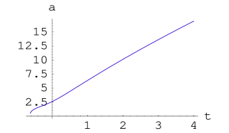
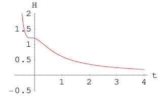
Figure 1: (Left panel) scale factor vs cosmic time $t$, (right panel) Hubble parameter $H$ vs $t$. The parameters are fixed at $c=3/\sqrt{7}$, $r_{c}=0.4$, $\tilde{b}=1$, $k=0$, $k_{1}=-1$.

From figures 1 and 2, we clearly see that the scale factor $a(t)$ can grow with $t$ much faster than the scale factor (or size) of the internal space $R_{c}~{}(\equiv r_{c}\times{f})$, where ,

$${f}={f}(\varphi(t))=\left(\frac{m(m-1)}{4}\right)^{1/(m+2)}\exp\left(\frac{2}{\sqrt{m(m+2)}}\,\frac{\varphi}{M_{P}}\right)$$ (27)

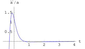
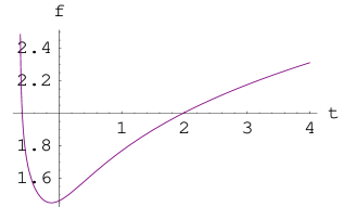
Figure 2: (Left panel) Acceleration $\ddot{a}/a$ vs cosmic time $t$, and (right panel) the growth factor $f\equiv{f}(\varphi(t))$, which measures the increase in the size (or scale factor) of the internal space with $t$. The parameter values are the same as the ones in Fig. 1.

The acceleration of the 4d universe is associated to a bounce of the compact internal space off its minimal scale factor (see also a discussion in [12]). Table 1 shows how the scale factor $a(t)$ and the term $f(\varphi(t))$ associated with the size of the internal space could vary with $t$, for a certain choice of initial conditions: $\varphi_{0}=0.5$, $\dot{\varphi}_{0}=0.5$ and $a_{0}=2.6$ . The other parameters are fixed at $k=0$, $k_{1}=-1$, $c=3/\sqrt{7}$ and $r_{c}=0.4$ . One also finds that for $t>>1$ (i.e., $\varphi>>1$), the flux contribution to the acceleration or the scale factor $a(t)$ of physical $3$-space is almost negligible, even if $\tilde{b}>>r_{c}^{-1}$, except for the case that $c\sim\sqrt{3}$.

Table 1: The scale factor $a(t)$ and $f(\varphi(t))$ as the function of proper time $t$.

	$t={10}^{2}$	$t={10}^{4}$	$t={10}^{6}$	$t={10}^{8}$
$a$	$2.1\times 10^{2}$	$7.2\times{10}^{3}$	$3.8\times{10}^{5}$	$8.6\times{10}^{6}$
${f}$	$4.7$	$13$	$35$	$100$

The combined effects of hyperbolic-flux compactification look different in many ways from the flux or hyperbolic compactification alone. This behavior can be seen also from the solutions presented in section 2. For example, if the curvature radius $r_{c}$ is sufficiently small and the flux parameter is $\tilde{b}\gtrsim r_{c}^{-1}$, then the acceleration parameter $\ddot{a}/a$, although negative, is almost zero for all $t$. That is, the deceleration following after a period of transient acceleration can be modest. In our model, for a spatially flat 4d universe ($k=0$), the acceleration is only a transient phenomenon for $c>1$ but it may be eternal for $c\leq 1$.

Some of the above discussions will, however, change if the spatial curvature of physical 3-space is negative. In this case, the cosmic acceleration may continue forever, even if $c>1$, when the background is triggered by non-trivial fluxes, like the parameter $\tilde{b}$, or by a higher dimensional cosmological constant. This observation is not totally new, which was made before in the work of Halliwell [19] but rather implicitly. We will discuss this effect more explicitly, in the presence of background flux, in subsection 2.4.

To deal with the late-time acceleration, there may be a need to introduce matter fields, since the (contemporary) universe contains about $30\%$ (baryonic plus dark) matter. But neither matter nor radiation contribution will make much difference to the amount of acceleration in these models, as it is clear from the relation $\dot{a}^{2}\propto a^{2}\,\rho_{R,M}+\mbox{constant}$, where $\rho_{M}\propto 1/a^{3}$ and $\rho_{R}\propto 1/a^{4}$; matter and radiation both satisfy the strong energy condition separately. The introduction of cold dark matter is phenomenologically well motivated and may be required for the construction of the effective 4d model nonetheless.

2.3 Toroidal flux compactification

For flat models (i.e., $k_{1}=0$ case) with a non-zero flux, we find it convenient to define

$$d\tau={\rm e}^{-(3/c)\varphi}\,dt\,,\quad\alpha(\tau)=\ln(a(t))\,.$$ (28)

Furthermore, with $k=0$, the field equations have the following form:

$$\varphi^{\prime\prime}-c\,{\varphi^{\prime}}^{2}+3{\alpha^{\prime}}{\varphi^{\prime}} = \frac{3\tilde{b}^{2}}{c}\,,$$ (29)

$$3{\alpha^{\prime}}^{2}-{\varphi^{\prime}}^{2} = \tilde{b}^{2}\,.$$ (30)

Especially, for $c\approx\sqrt{3}$, the solution is simple, which is given by

$${\rm e}^{\alpha(\tau)}\propto{\rm e}^{\tilde{b}^{2}\tau^{2}/4}\,\tau^{1/6}\,,\quad{\rm e}^{-\sqrt{3}\varphi}\propto{\rm e}^{-3\tilde{b}^{2}\tau^{2}/4}\,\tau^{1/2}\,.$$ (31)

This solution is accelerating in the interval $(\sqrt{3}-\sqrt{2})<\sqrt{6}\,\tilde{b}\,\tau<(\sqrt{3}+\sqrt{2})$. Clearly, the solution with $\tilde{b}>0$ is different from that with $\tilde{b}=0$, in the latter case there is no acceleration. By the same token, the $c\neq\sqrt{3}$ solution can be different from that with $c=\sqrt{3}$. For example, when $c=\sqrt{4/3}$ (i.e., $m=6$), the parametric solution is

$$\alpha^{\prime}=\frac{\tilde{b}\,(x^{2}+1)}{2\sqrt{3}\,x}\,,\quad\varphi^{\prime}=\frac{\tilde{b}\,(x^{2}-1)}{2\,x}\,,$$ (32)

where $x=x(\tau)$ satisfies the equation

$$\frac{c_{+}}{d_{+}}\,\tanh^{-1}\left(\frac{x}{d_{+}}\right)+\frac{c_{-}}{d_{-}}\,\tan^{-1}\left(\frac{x}{d_{-}}\right)=3\tau\tilde{b}\,,$$ (33)

with $c_{\pm}=4\sqrt{2}\pm 3\sqrt{3}$, $d_{\pm}=\sqrt{3\sqrt{6}\pm 7}$. The limit $x\to 0_{+}$ ($\varphi^{\prime}\to-\infty$) corresponds to $\tau\to 0_{+}$, while the limit $x\to 1$ ($\varphi^{\prime}\to 0$) corresponds to $\tau\sim 1/2\tilde{b}$. There is a transient acceleration when $x\to 1$. Similarly, for $c>\sqrt{3}$, there may arise a period of acceleration for the $k=-1$ cosmology (see also a related discussion in [2]).

2.4 Open universe and cosmic acceleration

The recent astronomical observations [1] appear to indicate that our observable universe is well described by flat Euclidean geometry. Does it mean that we shall study/construct only the spatially flat FLRW models and postpone investigation of open space cosmologies? The answer is perhaps not affirmative, since one cannot rule out the possibility of having a negatively curved four-dimensional universe in large distance scales, see, e.g., [28] .

Let us note that the most interesting case, $1<c<\sqrt{3}$, is an example of hyperbolic compactification which gives a power-law acceleration. To make our discussion more precise, we take $k=k_{1}=-1$ in the equations (16), (17) and set $b=0$. The background solution is

$$a_{0}=\frac{c\,t}{\sqrt{c^{2}-1}},\quad\varphi_{0}=\frac{1}{c}\,\ln\left({{M}ct}\right)\,.$$ (34)

Here the branch $c<1$ can be unstable due to an imaginary scale factor $a(t)$, so we require $c\gtrsim 1$  and hence $\Omega_{\varphi}\equiv 8\pi G\rho_{\varphi}/(3H_{0}^{2})=1-1/a_{0}^{2}H_{0}^{2}=1/c^{2}\lesssim 1$. The limit $c=1$ however may be approached once $\tilde{b}>0$. From (34), using $d\tau=e^{-c\,\varphi}\,dt$, we derive $t\propto{\exp}({{M}c\tau})$. In the limit $\tau>>{M}^{-1}$, so $t>>1$ and $\varphi>>1$, the contribution of the background fluxes to the potential is almost negligible. Indeed, since $\dot{\varphi}_{0}=1/(ct)$, the internal space never accelerates, rather its expansion rate decreases as $t$ advances (see also figure 3).

To lowest order, where $a=a_{0}+\delta a_{0}$ and $\varphi=\varphi_{0}+\delta\varphi_{0}$, the field equations take the following form:

$$\delta\ddot{\varphi}_{0}+3H_{0}\delta{\dot{\varphi}_{0}}+3\delta{H_{0}}\dot{\varphi_{0}}+{4M^{2}}c^{2}{\rm e}^{-2\,c\,\varphi_{0}}\delta{\varphi_{0}}=0$$ (35)

$$6H_{0}\delta{H_{0}}-2\dot{\varphi}_{0}\delta{\dot{\varphi}_{0}}+{4M^{2}}c{\rm e}^{-2c\,\varphi_{0}}\delta{\varphi_{0}}+\frac{6}{a_{0}^{2}}\,\frac{\delta{a_{0}}}{a_{0}}=0,$$ (36)

where $\delta H_{0}=-\,(\delta a_{0}/a_{0})\,H_{0}+\delta\dot{a}_{0}/a_{0}$. These equations have the solution

$$\delta a_{0}=\beta\,t^{n}\,,\quad\delta\varphi_{0}=\beta\gamma\,t^{n-1}\,,$$ (37)

where $\beta$ is undermined but a small constant, and

$$\gamma=\frac{3(1-n)}{4}\sqrt{c^{2}-1}\,,\quad n^{2}=\frac{4}{c^{2}}-3.$$ (38)

Thus, for $c<\sqrt{4/3}$, the acceleration tends to zero asymptotically, and there is no cosmological event horizon in this case. The behavior of the solutions (or trajectories in the phase portraits) may change at $c=\sqrt{4/3}$. In fact, the perturbative solution with $b=0$ may give an eternally accelerating expansion only if $m>6$ (i.e., $c<\sqrt{4/3}$) (which is in precise agreement with the earlier discussions in [19, 7]), while, for $c>\sqrt{4/3}$, the late-time acceleration can be oscillatory; this limit, however, can be pushed to $c>\sqrt{2}$ with $\tilde{b}>0$.

Let us take the point of view that a non-trivial flux (in extra dimensions) serves as a source term to lowest order perturbations of the scale factor and hence the late-time acceleration of the universe. In this case, the constant $\beta$ may be fixed in terms of $\tilde{b}$ and $M$, namely,

$$\beta={\tilde{b}^{2}}\,{M^{n-3}}\left(\frac{1}{\gamma}\right)\frac{(3n-1)(3-n)}{2n(3n^{2}+2n+3)}\,\left(\frac{3-n}{6}\right)^{1-n/2}\,,$$

$$\gamma=\frac{1-3n}{6(1-n)}\,\sqrt{9-n^{2}};~{}~{}\quad n=3(1-2/c^{2})\,.$$ (39)

The most suitable range turns out to be $1<c<\sqrt{2}$, and hence

$$0<\gamma<\sqrt{8/9}.$$

For $c=3/\sqrt{7}$ (i.e., $m=7$), one has $\gamma=\sqrt{7/8}$, $\beta\simeq 0.71\,\tilde{b}^{2}M^{-14/3}$. Here only the branch $c<\sqrt{2}$ is (eternally) accelerating. However, the full classical non-linear equations, with $\tilde{b}>0$, may still allow a power law acceleration for $c<\sqrt{3}$. Specifically, for $\tilde{b}\lesssim r_{c}^{-1}$, the universe starts to accelerate at early times and asymptotes to zero relatively quickly, while, for $\tilde{b}{\gg}r_{c}^{-1}$, it starts to accelerate only after a certain proper time, which may last for an infinitely long period before approaching a state of zero acceleration.

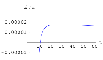
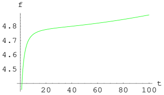
Figure 3: (Left panel) acceleration vs $t$, and (right panel) the growth factor $f\equiv{f}(\varphi(t))$ vs proper time ($t$). The parameters are fixed at $r_{c}=1$, $\tilde{b}=1$, $k=k_{1}=-1$ and $c=3/\sqrt{7}$. The initial values assigned at $t=0$ are $\varphi_{0}=0.5$, $\dot{\varphi}_{0}=0.6$ and $a=1$.

2.5 Compactification with a bulk cosmological term

From a pure gravity action with the $(4+m)$ dimensional cosmological term $\Lambda$, upon the dimensional reduction, we find that the 4d scalar potential is

$$V=-\,k_{1}{M_{P}^{2}}{{M}^{2}}\,{\rm e}^{-2c\,\frac{\varphi}{M_{P}}}+\frac{1}{2}\,\tilde{\Lambda}M_{P}^{2}\,{\rm e}^{-\,\frac{2}{c}\,\frac{\varphi}{M_{P}}}\,,$$ (40)

where $\tilde{\Lambda}\equiv\Lambda(4/m(m-1))^{1/c^{2}}$ with $m\geq 2$. The field equations then have the following form:

$$\ddot{\varphi}+3H\dot{\varphi}+{2c\,k_{1}}{{M}^{2}}\,{\rm e}^{-2c\,\varphi}-\frac{\tilde{\Lambda}}{c}\,{\rm e}^{-(2/c)\varphi}=0\,,$$ (41)

$$3H^{2}-\dot{\varphi}^{2}+{2k_{1}}{{M}^{2}}{\rm e}^{-2c\,\varphi}+\frac{3k}{a^{2}}-\tilde{\Lambda}{\rm e}^{-(2/c)\varphi}=0\,,$$ (42)

in units $\kappa=1$. Here the value $c=1$ is transitional. The consistency equation (18), which has no dependence on the flux parameter $b$, is the same. When $k=0$ and $k_{1}<0$ (again we take $k_{1}=-1$, for simplicity), we can find the exact solution for $c\approx 1$, which is given by

$$\sqrt{6}\,\alpha^{\prime}={M}\gamma\left(x+x^{-1}\right),~{}~{}\quad\sqrt{2}\,\varphi^{\prime}={M}\gamma\left(x-x^{-1}\right),$$

$$x\equiv\frac{\sqrt{3}+1}{\sqrt{2}}\,\tanh\left({M}\gamma\tau\right),~{}~{}\quad\gamma\equiv\sqrt{1+\frac{\tilde{\Lambda}}{2{M}^{2}}}$$ (43)

up to a shift of $\tau$ around $\tau=0$. Interestingly, this solution is accelerating for all $\tau$ satisfying

$$\tau>\sqrt{\frac{2}{2M^{2}+\tilde{\Lambda}}}\cosh^{-1}\sqrt{\frac{3+2\sqrt{3}}{6}}.$$ (44)

Acceleration is possible in the both cases $\Lambda>0$ and $\Lambda<0$, given that $\gamma>0$ holds. This translates to the condition that $\tilde{\Lambda}>-\,2{M}^{2}$. As in the case of form-field background, the accelerated expansion of a spatially flat universe can be eternal only if $c\leq 1$, otherwise the acceleration is transient. However, for the $k=-1$ cosmology, there can arise an eternally accelerating expansion even if $c\gtrsim 1$.

3 Compact hyperbolic manifolds and mass gap

Here we would like to elaborate a little more on the issue of size of the internal space and its associated mass gap. In our model, it may look somewhat disappointing that under the time-evolution not only the size of the physical 3-space but also the scale factor of the internal space expands. We argue that this itself is not a real problem, but instead may be a desirable feature if one really wants to achieve a slowly varying 4d scalar potential from the time-dependent string or M theory compactification on hyperbolic spaces.

In [10], it was argued that the $m_{KK}\sim 10^{-60}$ (in 4d Planck units), a value closer to the current Hubble scale $H_{0}\sim 10^{-33}~{}\mbox{eV}$, which is phenomenologically unacceptable. If so, the hyperbolic compactification in time-dependent background may be less attractive. Here we revisit the argument and show that it should be modified.

The mass gap discussed in [10] was based on the expectation that the Kaluza-Klein masses are bounded below by

$$m_{KK}={\cal O}(1)\,{\rm e}^{-(m+2)\phi/2}\,r_{c}^{-1}.$$ (45)

This estimate for a mass gap seemed to come from two more, somewhat independent, assumptions: firstly, the mass gap on a CHM is solely set by the scale $r_{c}^{-1}$, and secondly, in a (conformal) frame appropriate to the 4d observer, the metric is

$$d\hat{s}_{4+m}^{2}=g_{\mu\nu}(x)dx^{\mu}dx^{\nu}+r_{c}^{2}\,{\rm e}^{(m+2)\phi}d\Sigma^{2}_{m,k_{1}}.$$ (46)

These both points will require further scrutiny.

Let us recall that the metric solution that we have found (cf section 2) is

$$ds_{4+m}^{2}=e^{-m\phi}g_{\mu\nu}(x)dx^{\mu}dx^{\nu}+r_{c}^{2}\,{\rm e}^{2\phi}d\Sigma^{2}_{m,k_{1}}.$$ (47)

The difference between (46) and (47) is significant. In (47), the estimate for the size of the internal manifold as $r_{c}\,{\rm e}^{(m+2)\phi/2}$ is not four-dimensional, since here one is not going to a conformal frame appropriate to the 4d observer but instead to a $(4+m)$ metric spacetime conformally related to (46) . In addition, there is no a priori reason that $m_{KK}\sim\sqrt{V(\phi)}$ since the mass gap has anything to do with the eigenmode associated with the first linear eigenfunction on the (compact) internal manifold. In any case, we are not going to proceed in this manner.

Instead, we make the following observation. To evaluate a mass gap, one must write the metric applicable to a 4d observer. In doing this, the (conformal) factor $e^{-m\phi(t)}$ is absorbed while (dimensionally) reducing the term $\sqrt{-g_{4+m}}/G_{4+m}$ into $\sqrt{-g_{4}}/G_{4}$. The mass gap is then a product of the eigenvalue associated with first radial eigenfunction on the CH $m$-manifold times a suppression factor. To a 4d observer, this factor is simply

$${f}=\left(\frac{m(m-1)}{4}\right)^{1/(m+2)}\exp\left(\frac{2}{\sqrt{m(m+2)}}\,\frac{\varphi-\varphi_{0}}{M_{P}}\right).$$

It is known that in compact hyperbolic manifolds the first eigenvalue $\mu_{1}$ (associated with Laplace-Beltrami operator) cannot be bounded by either volume (specifically, $1/\mbox{Vol}(\Sigma)^{1/m}$) or the linear dimension  alone [29] (see also [24] which contain many of the points about the spectrum of the CHMs, including the fact that the gap is not given by the volume but by the linear diameter of the CHM, and that this could make the gap much bigger) .

In the zero-flux case, the geometric lower bounds on massive Kaluza-Klein excitations may be approximated, in the time-dependent background, by (see the appendix)

$$m_{KK}\sim\frac{{\cal O}(\pi)}{r_{c}\times{f}}.$$ (48)

The KK modes around $\varphi\sim\varphi_{0}$ can be extremely heavy, $m_{KK}\gtrsim{\cal O}(\pi)r_{c}^{-1}\simeq{M}\sim 10^{15}\,\mbox{GeV}$ and their number can be low $\simeq\frac{M_{P}^{2}}{{M}^{2}}\leq 10^{6}$.

The question arises as to whether it is possible to use M-theory motivated potential for dark energy, namely, $V(\varphi)\sim 10^{-120}\,M_{P}^{4}$. First, one might note that the Hubble parameter we measure is purely a 4d quantity, and so even the approximation $H\sim\sqrt{V}$ (assuming that $k=0$ and $\dot{\varphi}^{2}<<V(\varphi)$) may be valid only if one expresses the potential in terms of a canonically normalized 4d scalar $\varphi$. It is suggestive to analyze the results in terms of 4d cosmological parameters. For the M theory case, $m=7$, we have

$$V(\varphi)={{M}^{2}M_{P}^{2}}{\rm e}^{-\frac{6}{\sqrt{7}}\,\frac{\varphi-\varphi_{0}}{M_{P}}}+\frac{M_{P}^{2}\,\tilde{b}^{2}}{2}\,e^{-2\sqrt{7}\,\frac{\varphi-\varphi_{0}}{M_{P}}}.$$ (49)

For the tentative value $M\sim 10^{-3}M_{P}\sim 10^{15}\,\mbox{GeV}$, to get $V(\varphi)\sim 10^{-120}M_{P}^{4}$, we require $\varphi-\varphi_{0}\sim 115.7$ (in 4d Planck units) . This helps to estimate the growth factor ${f}$ by which the size of the compact internal space may have increased. To a 4d observer, the growth factor is ${f}\sim 6\times 10^{12}$ and hence $(r_{c}\times{f})^{-1}\sim 166\,{GeV}$, a mass gap that is physically interesting. It is plausible (but certainly not established) that when $V(\varphi)$ dropped from its Planck scale value $\sim 10^{66}\,(\mbox{GeV})^{4}$ to the current value $V\approx V_{0}=10^{-120}\,M_{P}^{4}$, the mass gap would decrease from $\sim 10^{15}\,\mbox{GeV}$ to ${\cal O}({10}^{2})\,\mbox{GeV}$.

Let us consider another example, which is based on the exact solution that we have presented in subsection 2.4. For $c=3/\sqrt{7}$, we easily compute

$${f}=\exp\left(\frac{2\,\varphi}{\sqrt{63}}\right)(10.5)^{1/9}\simeq{1.29}\ \left(\frac{3}{\sqrt{7}}\,{M}t\right)^{2/9}\,.$$ (50)

When $M=10^{-3}M_{P}$ and $t$ is as large as inverse of the present Hubble scale $t_{0}\sim H_{0}^{-1}\sim(10^{-33}\,\mbox{eV})^{-1}$, one finds $(r_{c}\times{f})^{-1}=R_{c}^{-1}\simeq 1.62\times 10^{11}\,\mbox{eV}\simeq 162~{}\mbox{GeV}$. This mass gap must clearly be considered tentative until the size of compactification around $\varphi\sim\varphi_{0}$, where ${f}\sim{\cal O}(1)$, or the curvature radius of internal space $r_{c}$ ($\equiv M^{-1}$) is known.

Of course, one could argue that even if $m_{KK}\sim\mbox{TeV}$ in these cases, one finds $m_{KK}<<\mbox{TeV}$ when $\varphi-\varphi_{0}>>115$ and $t>>t_{0}\equiv{10}^{33}(\mbox{eV})^{-1}$. The issue is whether we are willing to accept the value $V<<V_{0}\approx 10^{-120}M_{P}^{4}$. For example, in order to witness $m_{KK}\sim 10\,\mbox{GeV}$, we require ${f}\sim 10^{14}$ and hence $t\gtrsim 2.8\times{10}^{38}\,(\mbox{eV})^{-1}$, a time scale which is too large, like a few trillion years, and we may practically never approach this limit.

4 Discussion

In this paper, we have used the M-theory motivated scalar potentials to study the FRW type four dimensional flat (and open) universe cosmologies and shown that a scalar potential of the form $V\sim\Lambda_{1}\exp(-2c\kappa\varphi)+\Lambda_{2}\exp(-(6/c)\kappa\varphi)$ arising from the hyperbolic-flux compactification might be of interest for getting transiently or eternally accelerating expansion of the universe. For a spatially flat universe the accelerated expansion will continue forever only if the coupling $c\leq 1$, regardless of the background flux. In light of the result that for all known classical compactifications of supergravity theories on some non-trivial curved internal manifolds or toroidal spaces with trapped fluxes, only $c\gtrsim 1$ arises in practice, we are led to explore other alternatives for cosmic acceleration. We find that an eternally accelerating expansion is possible with $c>1$ if the spatial curvature of the universe is negative. For the case of hyperbolic compactification, this claim was made before in ref. [7] based on a result from linearized approximations. Here we have also generalized those results by solving the classical field equations with non-zero fluxes.

It is known, at least, for $m=2$ and $m=3$, that the most compact manifolds are hyperbolic. In the context of hyperbolic compactification, we point out that the existence of a mass gap in the ${\cal O}(10^{2})\,\mbox{GeV}$ is not impossible, since the curvature radius of the internal space can be extremely small, like $r_{c}\sim{\cal O}(10)M_{P}^{-1}$.

One direction of further investigation is to analyse the field equations as a dynamical system, in the manner of Halliwell, using a phase-plane method and see how the solutions behave in phase space asymptotically in the combined case of the hyperbolic-flux compactification. A step in this direction, with the settings $r_{c}=1$ and ${b}=0$, is recently taken in [30] (see also the last section of ref. [31]), which generalize the earlier phase-plane analysis in ref. [19].

Another direction is to extend our construction by taking some of the extra dimensions to be flat, like $T^{4}\times H^{3}/{\Gamma|_{free}}$, instead of the $H^{7}/\Gamma$ geometry, since the energy spectrum on a CH-$3$ manifold is better known as compared a CHM in four and higher-dimensions. In addition, every hyperbolic manifold $\Sigma_{m}=\mathbb{H}^{m}/\Gamma$ of finite volume, with $m\geq 3$, may be decomposed disjointedly into a relatively compact $\Sigma_{0}$ and many finite cusps. One may also include the brane (or brane-instanton) effects by allowing a delocalized flat transverse space. In this case, even though the flat part will have zero contribution to a scalar potential, the coupling constant $c$ will change. We hope to return to this and related problems elsewhere.

Appendix: Some useful results on CHMs

The eigenvalue equation $\left(\Delta_{LB}+\mu_{n}^{2}\right){\cal U}_{\mu}=0$ of the Laplace-Beltrami operator $\Delta_{LB}$ on a Riemannian manifold possessing both local geometry and global topology plays a significant role to set the scale of the metric perturbation. There may exist many bounds for the $n$th eigenvalue ${\mu_{n}}~{}(\equiv\sqrt{E_{n}}$) in terms of the diameter $d$ and the Ricci curvature $\tilde{R}$ of the manifold $\Sigma$ itself. For our purpose, it is crucial to know the behavior of low-lying eigenmodes.

As for m-dimensional compact hyperbolic manifolds, there are a number of estimates of $\mu_{1}(=\sqrt{E_{1}})$ in mathematical literature, see, e.g., [29]. If the Ricci curvature $\tilde{R}(\Sigma)$ is bounded below by $-\,(m-1)/l^{2}$, then $\mu_{1}(=\sqrt{E_{1}})$ satisfies

$$\mu_{1}^{2}\geq\mbox{max}\left[\frac{\pi^{2}}{2d^{2}}-\frac{1}{4l^{2}},\sqrt{\frac{\pi^{4}}{d^{4}}+\frac{1}{16l^{4}}}-\frac{3}{4l^{2}},\frac{\pi^{2}}{d^{2}}\exp\left(-c_{m}\frac{d}{2l}\right)\right],$$ (A.1)

where $c_{m}=\sqrt{2}$ if $m=2$ and $c_{m}=\sqrt{m-1}$ if $m\geq 3$. $\mu_{1}$ determines the maximum fluctuation scale of the perturbation and hence the geometric lower bound on KK masses. If $d$ is larger than $\sqrt{2}\pi l$, then $E_{1}>0$ but it does not say anything about the existence of modes $\mu<1/r_{c}$. At any rate, since $\mbox{Vol}(\Sigma)\sim r_{c}^{m}e^{\alpha}$, it is clear that the first eigenvalue $\mu_{1}$ cannot be bounded by either volume or the diameter alone.

It is also known that, for $m\geq 2$, there exist upper bounds to the eigenvalues $\mu_{n}$ (counted with multiplicity, $0=\mu_{0}(\Sigma)<\mu_{1}(\Sigma)\leqq\mu_{2}(\Sigma)\leqq\cdots$) [29] (there is an incorrect sign in [32])

$$\mu_{n}^{2}\leq\left\{\begin{array}[]{l}\frac{4\pi^{2}n^{2}}{d^{2}}\left(1+2^{(m-2)/2}\right)^{2}+\frac{(m-1)^{2}}{4\,l^{2}},\quad(m=\mbox{even}),\\ \frac{4(1+\pi^{2})n^{2}}{d^{2}}\left(1+2^{m-3}\right)^{2}+\frac{(m-1)^{2}}{l^{2}},\quad(m=\mbox{odd}).\end{array}\right.\$$ (A.4)

$\mu_{1}$ may be arbitrarily close to zero if $m=2$. This is understandable because one can deform a CH$-2$ manifold continuously so that $d\to\infty$. For CHM with $m\geq 3$, this is prohibited and by Mostow-Prasad rigidity theorem there are no massless shape moduli [24]. For the $m=3$ case, a more useful empirical relation is the Weyl formula:

$${\mu}_{1}=\sqrt{\frac{1}{r_{c}^{2}}+\left(\frac{9\pi^{2}}{\mbox{Vol}(\Sigma)}\right)^{2/3}}.$$ (A.5)

The mass gap can much larger than $(\mbox{Vol}(\Sigma))^{-1/m}$ when the ‘complexity’ of the manifold (i.e., the $m$-dimensional generalization of the genus) is large. The above relation was found in close agreement with a numerical result for “smallest” $263$ CH-$3$ manifolds [33].

In the limit $d>>r_{c}/2$, where the manifold converges to the original cusped manifold and $\mu_{1}(\mbox{cusp})\sim 1/r_{c}$ , one has

$$\mu_{1}=\sqrt{(\mu_{1}(\mbox{cusp}))^{2}+\frac{4\pi^{2}}{\beta^{2}d^{2}}},$$

and $\mbox{Vol}(\Sigma)\simeq\mbox{Vol}(\Sigma_{\mbox{cusp}})[1-\exp(-2(d-d_{0}))]$ where $d\geqq d_{0}=0.25\,r_{c}$. Here $d_{0}$ is the diameter of the complementary part to that of a ‘thin’ part. One may cut the neighborhood of a cusp (or ‘thin’ part), so that $d_{0}$ becomes the usual diameter. This relation holds for some manifolds with one ‘thin’ part (see [33] and references therein). The numerical results in [33] also suggest that for ‘smallest’ CH-$3$ manifolds $\langle\beta\rangle=1.7$, although for each manifold the value of $\beta$ may be different, e.g., $\beta=1.3$ is the value for a specific manifold.

Another method to compute the eigenvalues (in terms of periodic orbits) is the Selberg trace formula, e.g., for CH-$2$ manifold, $\mu_{1}>0.47/r_{c}$ (see, e.g. [24] and references therein). This method has not been used to any CHMs with $m\geq 3$. The Weyl asymptotic formula that generally holds for modes with $\mu_{1}>>1/r_{c}$ gives the number density of KK states:

$${\cal N}(\mu)\sim\frac{1}{(2\pi)^{m}}\,\Omega_{m}\mbox{Vol}(\Sigma_{m})\mu^{m},$$

where $\Omega_{m}=2\pi^{m/2}/(m\,\Gamma(m/2))$ is the volume of the unit disk in a Euclidean $m$-space. The formula written in [24] (cf equation (8)) may give a good approximation for CHMs that extend in one direction, i.e., $d>>r_{c}/2$.

There can be only a lower bound to the volume of compact hyperbolic space, like $V_{CH3}>0.1667\,r_{c}^{3}$, and the known example with smallest volume is Weeks manifold with $V>0.94\,r_{c}^{3}$. For some specific $m=2$ or $m=3$ CH manifolds, it often happens that $e^{\alpha}\sim{\cal O}(1)$. In general, however, the quantity $e^{\alpha}$ is arbitrary, which is essentially a counting of the number of handles on the CH manifold . If one allows the internal space to be compact hyperbolic orbifolds then the volume can be much smaller, see, e.g.,[34].

References

- [1] A. Riess et.al., Astron. J. 117 (1999) 707; D.N. Spergel et.al. Astrophys. J. Suppl. 148 (2003) 175, arXiv:astro-ph/0302209; S. Perlmutter et.al., astro-ph/0309368.
- [2] L. Cornalba and M.S. Costa, A new cosmological scenario in String theory, Phys. Rev. D 66 (2002) 066001 [hep-th/0203031].
- [3] P. K. Townsend and M.N.R. Wohlfarth, Accelerating cosmologies from compactification, Phy. Rev. Lett. 91 (2003) 061302 [hep-th/0303097].
- [4] C.-M. Chen, P.-M. Ho, I. P. Neupane, and J. E. Wang, A Note on Acceleration from Product Space Compactification, JHEP 0307 (2003) 017 [hep-th/0304177].
- [5] N. Ohta, Accelerating cosmologies from S-branes, Phy. Rev. Lett. 91 (2003) 061303 [hep-th/0303238].
- [6] R. Emparan and J. Garriga, A note on accelerating cosmologies from compactifications and S-branes, JHEP 0305 (2003) 028 [hep-th/0304124].
- [7] C.-M. Chen, P.-M. Ho, I. P. Neupane, N. Ohta, and J. E. Wang, Hyperbolic Space Cosmologies, JHEP 0310 (2003) 058 [hep-th/0306291].
- [8] M.N.R. Wohlfarth, Accelerating cosmologies and a phase transition in M-theory, Phys. Lett. 563 (2003) 1 [hep-th/0304089].
-
[9]
N. Ohta, A study of accelerating cosmologies from
Superstring/M-theory, Prog. Theor. Phys. 110 (2003)
269 [hep-th/0304172];
S. Roy, Accelerating cosmologies from M/String-theory, Phys. Lett. B567 (2003) 322 [hep-th/0304084]. - [10] M. Gutperle, R. Kallosh and A. Linde, M/String theory, S-branes and accelerating universe, JCAP 0307 (2003) 001 [hep-th/0304225].
- [11] M.N.R. Wohlfarth, Inflationary cosmologies from compactification, Phys. Rev. D 69 (2004) 066002 [hep-th/0307179].
- [12] P. K. Townsend, Cosmic acceleration and M theory, hep-th/0308149.
- [13] I. P. Neupane, Inflation from string/M-theory compactification, hep-th/0309139.
- [14] L. Järv, T. Mohaupt and F. Saueressig, M-theory cosmologies from singular Calabi-Yau compactifications, hep-th/0310174.
-
[15]
G. W. Gibbons, Aspects of supergravity
theories, GIFT Seminar 1984, pp. 123-146,
(QCD161:G2:1984), also in Supersymmetry, supergravity and
related topics, World Scientific, 1985;
J.M. Maldacena and C. Nunez, Supergravity description of field theories on curved manifolds, and a no-go theorem, Int. J. Mod. Phys. A16 (2001) 822 [hep-th/0007018]. - [16] S. Kachru, R. Kallosh, A. Linde, and S.P. Trivedi, De Sitter vacua in string theory, Phys. Rev. D 68 (2003) 046005 [hep-th/0301240].
- [17] S. B. Giddings, The fate of four dimensions, Phys. Rev. D 68 (2003) 026006 [hep-th/0303031].
- [18] S. Kachru, R. Kallosh, A. Linde, J. Maldacena, L. McAllister, and S.P. Trivedi, Towards inflation in string theory, JCAP 0310 (2003) 013 [hep-th/0308055].
- [19] J. J. Halliwell, Scalar fields in cosmology with an exponential potential, Phys. Lett. B 185 (1987) 341.
- [20] B. Ratra and P.J.E. Peebles, Cosmological consequences of a rolling homogeneous scalar field, Phys. Rev. D 37 (1988) 3406.
-
[21]
J. Yokoyama and K.-I. Maeda, On the dynamics
of the power law inflation due to an exponential potential,
Phys. Lett. B 207 (1988) 31;
A.A. Coley, J. Ibanez, and R.J. van den Hoogen, Homogeneous scalar field cosmologies with an exponential potential, J. Math. Phys. 38 (1997) 5256. - [22] V.D. Ivashchuk, V.N. Melnikov, and A.B. Selivanov, Cosmological solutions in multidimensional model with multiple exponential potential, JHEP 0309 (2003) 059.
-
[23]
T. Barreiro, E.J. Copeland, and N.J. Nunes,
Quintessence arising from exponential potentials,
Phys. Rev. D 61 (2000) 127301 [astro-ph/9910214];
A.A. Sen and S. Sethi, Quintessence model with double exponential potential, Phys. Lett. B 532 (2002) 159 [gr-qc/0111082];
U. Franca and R. Rosenfeld, Fine tuning in quintessence models with exponential potential, JHEP 0210 (2002) 015 [astro-ph/0206194]. -
[24]
N. Kaloper, J. March-Russell, G.D. Starkman, and
M. Trodden, Compact hyperbolic extra dimensions: branes,
Kaluza-Klein modes and cosmology, Phys. Rev. Lett.
85 (2000) 928 [hep-ph/0002001].
G.D. Starkman, Dejan Stojkovic, and M. Trodden, Large extra dimensions and cosmological problems, Phys. Rev. D 63 (2001) 103511 [hep-th/0012226]. - [25] C.-M. Chen, D. V. Galtsov, and M. Gutperle, S brane solutins in supergravity theories, Phys. Rev. D 66 (2002) 024043 [hep-th/0204071]; N. Ohta, Intersecting rules for S-branes, Phys. Lett. B 588 (2003) 213 [hep-th/0301095].
- [26] C. P. Burgess, C. Núñez, F. Quevedo, G. Tasinato, and I. Zavala, General brane geometries from scalar potential, gauged supergravities and accelerating universes, JHEP 0308 (2003) 056 [hep-th/0305211].
- [27] P.K. Townsend, Private communication (2003).
-
[28]
C. Rubano, P. Scudellaro, S. Capozziello, and M. Capone,
Exponential potentials for tracker fields, arXiv:astro-ph/0311537;
T. Roy Choudhury and T. Padmanabhan, A theorertician’s analysis of the supernova data and the limitations in determining the nature of dark energy II: results for latest data, arXiv:astro-ph/0311622. - [29] S.-Y. Cheng, Eigenvalue comparison theorems and its geometric applications, Math. Z. 143 (1975) 289; X. Cheng and D. Zhou, “First eigenvalue estimate on Riemannian manifolds”, Hokkaido Mathematical J. 24 (1995) 453.
- [30] P. G. Vieira, Late-time cosmic dynamics from M-theory, arXiv:hep-th/0311173.
- [31] L. Cornalba and M. S. Costa, Time dependent orbifolds and string cosmology, arXiv:hep-th/0310099.
- [32] A. Mukherjee and R. Tabbash, Geometric bounds on Kaluza-Klein masses, Eur. Phys. J. C 20 (2001) 193.
- [33] K. T. Inoue, Numerical study of length spectra and low-lying eigenvalue speactra of compact hyperbolic -manifolds, Class. Quant. Grav. 18 (2001) 629 [math-ph/0011012]; arXiv:astro-ph/0103158 (PhD Thesis).
- [34] K.T. Inoue, Computation of eigenmodes on a compact hyperbolic space, Class. Quant. Grav. 16, (1999) 3071 [astro-ph/9810034].