Degenerate BPS Domain Walls:
Classical and Quantum Dynamics

Abstract

We discuss classical and quantum aspects of the dynamics of a family of domain walls arising in a generalized Wess-Zumino model. These domain walls can be embedded in ${\cal N}=1$ supergravity as exact solutions and are composed of two basic lumps.

1 Introduction

Currently the topic of supersymmetric extended objects is extremely fashionable. Before the advent of the new brane world, however, only a few workers paid attention to the physical and mathematical properties of super-membranes of various dimensions. Among such pioneers, we mention the work on the cohomological interpretation of the topological charges associated with these extended objects by J. A. de Azcarraga and collaborators, see [2]. Relevant contributions to the subject can be found also in the work of M. Cvetic, S. J. Rey et al, [3]. In this paper, we offer a brief summary of our work on a related topic -the dynamics of BPS domain walls- to honor Adolfo, Professor and friend to several of us from the Salamanca years circa 1977.

We focus on a generalized Wess-Zumino model with two ${\cal N}=1$ chiral superfields, first discussed by Bazeia et al. in Reference [4]. Slightly later in [5], it was shown by Shifman and Voloshin that this model admits a degenerate family of BPS domain walls. The general variety of both non-BPS and BPS solitary waves has been described in [6], studying the (1+1)-dimensional version of the system. More recently, Eto and Sakai, see [7], have discovered how to define a “local” superpotential in such a way that the domain walls of the generalized Wess-Zumino model remain exact solutions in ${\cal N}=1$ (3+1)-dimensional supergravity.

A remarkable feature of this supersymmetric system is the availability of analytic descriptions of the domain wall dynamics along orthogonal lines to the “two”-branes. BPS wall/BPS anti-wall dynamics have been discussed in [8], analyzing the energy density of non-BPS wall/anti-wall configurations. In [9], however, several of us unveiled the adiabatic dynamics of BPS two-walls by studying geodesic motion in the moduli space. The dynamics inside the wall at low energy is ruled by the “effective action”, see [10], governing the evolution of Goldstone bosons through the two-brane. Although Lorentz invariance forbids dependence on the center of mass of the wall, in our system with two real scalar fields the effective action depends on the relative coordinate that labels the distance between walls; the inertia for Goldstone bosons running either on distant or intersecting walls are different, smoothly varying from one to another.

The above results concerning the classical dynamics of domain walls are based on a crucial property: the degeneracy of the classical moduli space of domain walls. The question arises as to whether this degeneracy survives quantum fluctuations. Analyse of the one-loop fluctuations around the wall solutions in the “body” of the supersymmetric system reveal that repulsive forces, decaying exponentially with distance, arise between the fundamental lumps, see [11]. However, a general theorem warranting the identity between the one-loop corrections to kink masses and the anomaly in the central charge of the ${\cal N}=1$ SUSY algebra, see e.g. [12], tells us that at the quantum level wall degeneracy occurs in the fully supersymmetric system.

2 Moduli space of solitary waves in generalized
Wess-Zumino models

We shall consider the (3+1)-dimensional ${\cal N}=1$ supersymmetric Wess-Zumino model, where the superpotential

$$W^{3D}(\Phi_{1},\Phi_{2})={4\over 3}\Phi_{1}^{3}-\Phi_{1}+2\sigma\Phi_{1}\Phi_{2}^{2}$$

determines the interactions between the two chiral superfields: $\Phi_{1}(x^{0},\vec{x},\theta_{\alpha}),\ \ \Phi_{2}(x^{0},\vec{x},\theta_{\alpha})$ . Here, the four-vectors $x^{\mu}=(x^{0},\vec{x})$ and the Grassman Weyl spinors $\theta_{\alpha}$ provide (non-dimensional) coordinates in ${\cal N}=1$ Minkowski superspace. $\sigma$ is the only (non-dimensional) coupling constant.

In our search for domain walls, we need to explore only the “body” of the theory, i.e. we shall focus on the first terms of the Grassman expansion of the fields and the superpotential: $\Phi_{1}|_{\theta_{\alpha}=0}=\phi_{1}+i\psi_{1},\ \ \Phi_{2}|_{\theta_{\alpha}=0}=\phi_{2}+i\psi_{2}$. Moreover, the reality condition $\psi_{1}=\psi_{2}=0$ and the requirement of independence of the $(y,z)$ variables (dimensional reduction), $\phi_{1}(x^{0},\vec{x})=\phi_{1}(x^{0},x),\ \ \phi_{2}(x^{0},\vec{x})=\phi_{2}(x^{0},x)$, lead us to the (1+1)-dimensional superpotential:

$$W(\phi_{1},\phi_{2})={1\over 2}{\rm Re}W^{3D}(\phi_{1}(x^{0},x),\phi_{2}(x^{0},x))={1\over 2}\left[{4\over 3}\phi_{1}^{3}-\phi_{1}+2\sigma\phi_{1}\phi_{2}^{2}\right].$$

Therefore, the domain walls of the original Wess-Zumino model are in one-to-one correspondence with the solitary waves (kinks) of the (1+1)-dimensional system, with dynamics governed by the action:

$$S=\int\,d^{2}x\left[{1\over 2}\partial_{\mu}\phi_{1}\partial^{\mu}\phi_{1}+{1\over 2}\partial_{\mu}\phi_{2}\partial^{\mu}\phi_{2}-{1\over 2}{\partial W\over\partial\phi_{1}}{\partial W\over\partial\phi_{1}}-{1\over 2}{\partial W\over\partial\phi_{2}}{\partial W\over\partial\phi_{2}}\right]\ .$$ (1)

The vacuum moduli space, characterized as the set of critical points of $W$ modulo the internal parity symmetry group of the problem, contains the “two” points: $(\phi_{1}^{V_{1}^{\pm}}=\pm{1\over 2}\ ,\ \phi_{2}^{V_{1}^{\pm}}=0)$ , $(\phi_{1}^{V_{2}^{\pm}}=0\ ,\ \phi_{2}^{V_{2}^{\pm}}=\pm{1\over\sqrt{2\sigma}})$.

2.1 The search for Kinks

We shall focus only on the topological sector connecting the $V_{1}^{\pm}$ vacua. Generically, solitary waves in other topological sectors are not BPS kinks; the problem of kink stability is studied in [13] from a geometrical point of view. The energy for static configurations can be written à la Bogomolny, resulting in:

$$E(\phi_{1},\phi_{2})={1\over 2}\int\,dx\left[\left({d\phi_{1}\over dx}-{\partial W\over\partial\phi_{1}}\right)^{2}+\left({d\phi_{2}\over dx}-{\partial W\over\partial\phi_{2}}\right)^{2}\right]+\int_{P}\,\left[d\phi_{1}{\partial W\over\partial\phi_{1}}+d\phi_{2}{\partial W\over\partial\phi_{2}}\right].$$ (2)

Given a polynomial superpotential such as $W$, the solutions of the first-order equations

$${d\phi_{1}\over dx}={\partial W\over\partial\phi_{1}}\qquad,\qquad{d\phi_{2}\over dx}={\partial W\over\partial\phi_{2}}$$ (3)

are absolute minima of $E$, usually referred to as BPS kinks that saturate the topological bound: $E_{T}=\int_{P}\,dW=|W(+\infty)-W(-\infty)|$ .

From (3), the flow lines of ${\rm grad}W$ are identified as the solutions of the ODE:

$${d\phi_{1}\over d\phi_{2}}={4\phi_{1}^{2}+2\sigma\phi_{2}^{2}-1\over 4\sigma\phi_{1}\phi_{2}}\ .$$

There is an integrating factor, $|\phi_{2}|^{-({2\over\sigma}+1)}$ if $\sigma\neq 0$, $\sigma\neq 1$, and the flow lines -Kink orbits- are the curves:

$$\phi_{1}^{2}+{\sigma\over 2(1-\sigma)}\phi_{2}^{2}={1\over 4}+{c\over 2\sigma}|\phi_{2}|^{{2\over\sigma}}\qquad,$$ (4)

where $c\in(-\infty,c^{S}=\frac{1}{4}\frac{\sigma}{1-\sigma}\left(2\sigma\right)^{\frac{\sigma+1}{\sigma}})$ is an integration constant.

The meaning of these solutions can be summarized as follows: there are two maxima of $-U(\phi_{1},\phi_{2})$ with the same height. Kink solutions which pass from one maximum to the other depend on a parameter, $c$, which measures whether the particle moves through the bottom of the valley or more along the sides on the curve (4). There is a critical value $c^{S}$ of $c$ where the particle moves as high as possible; when $c$ increases beyond this critical value the particle crosses the mountain and falls off to the other side, see Figure 1.

                             

Figure 1: The $-U(\phi)=-{1\over 2}{\partial W\over\partial\phi_{1}}{\partial W\over\partial\phi_{1}}-{1\over 2}{\partial W\over\partial\phi_{2}}{\partial W\over\partial\phi_{2}}$ potential (left) Flow-lines: in the ranges $c\in(-\infty,c^{S})$ (middle left), $c=c^{S}$ (middle right), and $c\in(c^{S},\infty)$ (right).

Exactly at the critical value, the kink orbit starts at the point $\vec{\phi}^{V_{1}^{\pm}}$ and ends at the other point $\vec{\phi}^{V_{2}^{\pm}}$; this is in contrast to any other kink orbit for $c<c^{S}$, which starts at $\vec{\phi}^{V_{1}^{\pm}}$ but ends in $\vec{\phi}^{V_{1}^{\mp}}$. Thus, there are two kinds of kinks living in different topological sectors of the system: “link” kinks, interpolating between different points of the vacuum moduli space, and “loop” kinks, joining vacua identified as the same point of the vacuum moduli.

To find the kink form factors, one plugs formula (4) into (3) so that the problem is reduced to solving the quadrature:

$$I[\phi_{2}]=\int\frac{d\phi_{2}}{\phi_{2}\sqrt{\frac{1}{4}+\frac{c}{2\sigma}|\phi_{2}|^{\frac{2}{\sigma}}-\frac{\sigma}{2(1-\sigma)}\phi_{2}^{2}}}=2\sigma(x+a)=z$$ (5)

$$\phi_{1}^{{\rm TK}2}[x;a,c]=\pm\sqrt{\frac{1}{4}+\frac{c}{2\sigma}|I^{-1}(z)|^{\frac{2}{\sigma}}-\frac{\sigma}{2(1-\sigma)}[I^{-1}(z)]^{2}}\quad,\quad\phi_{2}^{{\rm TK}2}[x;a,c]=I^{-1}(z)$$

2.2 Special cases: Liouville systems

Explicit analytic integration of (5) in terms of elementary functions is only possible if $\sigma=2$ and $\sigma={1\over 2}$. The reason is that the analogous mechanical problem that one needs to solve in the search for one-dimensional solitary waves is an integrable Liouville system. Also, when $\sigma=3,4,{1\over 3}$ and ${1\over 4}$, the quadrature can be found analytically, but in these cases one is forced to deal with elliptic functions.

We present the analytic outcome of finding $I$ and its inverse $I^{-1}$ in the two Liouville cases. In Figure 2 we show kink profiles for several values of $b$ and $\sigma={1\over 2}$.

$\bullet$ ${\bf\sigma}=2$

$$\phi_{1}^{{\rm TK2}}[x;a,b]=\frac{(-1)^{\alpha}}{2}\frac{\sinh 4(x+a)}{\cosh 4(x+a)+b}\hskip 28.45274pt\phi_{2}^{{\rm TK2}}[x;a,b]=\frac{(-1)^{\beta}}{2}\frac{\sqrt{b^{2}-1}}{\cosh 4(x+a)+b}\qquad,$$

where $\alpha,\beta=0,1$, and $a\in{\mathbb{R}}$ is the center of the kink. The parameter $b$ is related to the integration constant as follows: $b=\frac{-c}{\sqrt{c^{2}-16}}$, so that $b\in(1,\infty)$.

$\bullet$ ${\bf\sigma}=\frac{1}{2}$

$$\phi_{1}^{{\rm TK2}}[x;a,b]=\frac{(-1)^{\alpha}}{2}\frac{\sinh(x+a)}{\cosh(x+a)+b^{2}}\hskip 28.45274pt\phi^{{\rm TK2}}_{2}[x;a,b]=(-1)^{\beta}\frac{b}{\sqrt{b^{2}+\cosh(x+a)}}\quad.$$ (6)

Again, $a\in{\mathbb{R}}$ is the kink center, $b$ is related to $c$ as $b^{2}=\frac{1}{\sqrt{1-4c}}\in(0,\infty)$, $\alpha,\beta=0,1$.

Figure 2: Solitary waves for $\sigma={1\over 2}$ corresponding to: (a) $b=0$, (b) $b=\sqrt{0.5}$, (c) $b=1$ and (d) $b=\sqrt{30}$.

2.3 Moduli space of BPS kinks

To elucidate the physical meaning of the $b$ parameter, we focus on the $\sigma=\frac{1}{2}$ case because it provides an analytical description of the generic behaviour. In Figure 3, pictures of the energy density are depicted for the same kinks shown in Figure 2. Note that for $b^{2}>1$ the energy density presents two lumps, whereas if $b^{2}<1$ the density is of the usual bell-shaped form. Also, because changing $b$ to $-b$ in the solution is equivalent to changing $\phi_{2}$ to $-\phi_{2}$ and the energy density is not sensitive to the sign of $b$, it is sensible to describe the moduli space of kinks as the half-plane parametrized by the $(a,b^{2})$ coordinates: $a$ fixes the center of mass of the two lumps, and $b^{2}$ can be interpreted as the relative coordinate that measures the distance between them.

Figure 3: Energy density ${\cal E}^{K}[x;0,b]$ for (a) $b=0$, (b) $b=\sqrt{0.5}$, (c) $b=1$ and (d) $b=\sqrt{30}$.

This qualitative description can be precisely established in an analytic fashion by looking at the maxima of the energy density ${\cal E}^{K}[x;a,b]$. These can be found through a classical analysis, applying the Cardano and Vieta formulas and Rolle’s theorem. We obtain the following conclusions:

1. If $b^{2}\in[0,1]$, $x=0$ is the only critical point (maximum) of ${\cal E}^{K}$ and ${\cal E}^{K}[0;0,b]={2\over(b^{2}+1)^{2}}$. Therefore, $b^{2}$ measures the height of ${\cal E}^{K}$ in this regime where the two lumps are aggregate.

2. If $b^{2}\in(1,\infty)$, $x=0$ is a minimum. Because ${\partial{\cal E}^{K}\over\partial x}[x;0,b]={2{\rm sinh}x\over[b^{2}+{\rm cosh}x]^{5}}P_{3}[{\rm cosh}x]$, where $P_{3}[{\rm cosh}x]$ is a third order polynomial with real roots $\pm\sqrt{r(b^{2})}$, see [9], we identify $x=\pm m(b^{2})=\pm{\rm arccosh}[1+r(b^{2})]$ as the two maxima of ${\cal E}^{K}$ obeying to the peak of the energy density of the two lumps. $b^{2}$ measures (in a highly non-linear scale set by the known function $r(b^{2})$) the distance between lumps.

3 Low-energy classical dynamics of BPS domain walls

In this section, we recover the (3+1)-dimensional point of view where our kinks become domain walls. The aim is to study the low-energy classical dynamics of these BPS topological walls, which can be understood as composed of the two basic link walls. We shall focus on the $\sigma=\frac{1}{2}$ case, for which analytical formulas are available.

3.1 Adiabatic motion orthogonal to the wall

We first analyze the motion orthogonal to the wall. In the case of walls grown from kinks of a single real scalar field, this analysis is not necessary because Lorentz invariance takes care of the matter. Besides the $a$ coordinate, describing the motion of the wall center of mass in the orthogonal direction ruled by Lorentz symmetry, there is another parameter in the moduli space of domain walls: the relative coordinate $b$. The dynamics of the motion on the $b$-coordinate along the $x$-axis is non-trivial; the dependence of $b$ on time precisely characterizes how the two basic walls intersect and split on their way along the $x$-axis.

Starting from the Hamiltonian of the reduced system,

$$H[\phi_{1},\phi_{2},\dot{\phi_{1}},\dot{\phi_{2}}]=\int\,dx{1\over 2}\left({\partial\phi_{1}^{K}\over\partial x^{0}}{\partial\phi_{1}^{K}\over\partial x^{0}}+{\partial\phi_{2}^{K}\over\partial x^{0}}{\partial\phi_{2}^{K}\over\partial x^{0}}\right)+\int\,dx\,{\cal E}\qquad,$$

we apply the adiabatic hypothesis of Manton [14] to study the low-energy dynamics of topological defects as geodesic motion in the moduli space. The smooth evolution on the moduli hypothesis

$$\phi_{1}^{K}(x^{0},x)=\phi_{1}^{K}[x;a(t),b(t)]\qquad,\qquad\phi_{2}^{K}(x^{0},x)=\phi_{2}^{K}[x;a(t),b(t)]$$

is plugged into the action and, after integrating out the $x$ variable, we find that $S$ becomes the action for geodesic motion in the kink moduli space with a metric inherited from the dynamics of the zero modes:

$$S=\int dt\left\{\frac{1}{2}g_{aa}(a,b)\frac{da}{dt}\frac{da}{dt}+g_{ab}(a,b)\frac{da}{dt}\frac{db}{dt}+\frac{1}{2}g_{bb}(a,b)\frac{db}{dt}\frac{db}{dt}\right\}.$$

The components of the metric tensor are: $g_{aa}(a,b)=\frac{1}{3},\ g_{ab}(a,b)=0,\ g_{bb}(a,b)=\frac{1}{3}h(b)$, where

$$h(b)=\frac{1}{4(b^{4}-1)^{2}}\left[2b^{6}-5b^{2}+3\frac{\arctan\left(\frac{\sqrt{1-b^{4}}}{b^{2}}\right)}{\sqrt{1-b^{4}}}\right]\quad.$$ (7)

As expected, the metric is independent of the center of mass $a$. Despite appearances, the behaviour of the metric is regular in the transition of $b^{2}$ from lower to higher values than 1. For a metric of the form given, the geodesics are easily found: they are merely straight lines on the $a-{\bar{b}}$ plane:

$$a(t)=k_{1}t+k_{2}\qquad,\qquad{\bar{b}}(t)=k_{1}^{\prime}t+k_{2}^{\prime}=\int\,db\sqrt{h(b)}\qquad.$$ (8)

$k_{1}$, $k_{2}$, $k_{1}^{\prime}$ and $k_{2}^{\prime}$ are integration constants. It is worthwhile to use (8) to express the geodesic orbits in the kink space:

$${\bar{b}}=\int\,db\sqrt{h(b)}=\kappa_{1}a+\kappa_{2}\qquad,\quad\kappa_{1}={k_{1}^{\prime}\over k_{1}}\quad,\quad\kappa_{2}=k_{2}^{\prime}-\kappa_{1}k_{2}$$ (9)

There are two main types:

$\bullet$ Choosing $\kappa_{1}=0\equiv b={\rm constant}$ in (9) we obtain geodesics describing free motion of the center of mass without any variation in separation of the two lumps, see Figure 4.

Figure 4: Energy density evolution along straight geodesic lines with $b$=constant: (a) $b=0.9$, a single lump is moving (b) $b=10$, synchronous motion of two lumps. Time runs from left to right.

$\bullet$ If we choose $\kappa_{1}\neq 0$ the geodesics also describe a non-trivial motion of the relative coordinate. A MATHEMATICA numerical plot choosing $\kappa_{1}=3$, $\kappa_{1}=2$, $\kappa_{1}=1$ whereas $\kappa_{2}$ is fixed by setting $b=0.1$ at $t=-{k_{2}\over k_{1}}$ is shown in Figure 5(a). Clearly, these geodesics describe exact solutions at the adiabatic limit for intersecting walls. There is analogy with the scattering of solitons in the sine-Gordon model, although, in this case, shape-preserving collisions only occur in the topological sector with a loop kink. As compared with similar phenomena, we find hybrid behaviour in our system between the sine-Gordon and $\lambda(\phi^{4})_{2}$ models.

         

Figure 5: (a) Evolution of energy density along a generic geodesic curve. (b) Plot of the functions $f^{2}(b)$ (up) and $f^{1}(b)$ (down).

3.2 Effective action for intersecting walls

The effective action for domain walls modeled on kinks without internal structure is derived by expanding the action around the classical solution and taking into account only the zero mode in the direction orthogonal to the wall, see [10]. We proceed along the same way to unveil the effective action induced by the zero modes for intersecting walls. There are two zero modes in the direction orthogonal to these composite two-branes. The collective coordinates corresponding to these zero modes are precisely the coordinates of the kink moduli space.

The Hessian driving the small fluctuations orthogonal to the domain wall is

$${\cal K}=\left(\begin{array}[]{cc}\frac{d^{2}}{dx^{2}}-\frac{3b^{2}}{\cosh x+b^{2}}-\frac{6\sinh^{2}x}{(\cosh x+b^{2})^{2}}+2&\frac{-6b\sinh x}{(\cosh x+b^{2})^{\frac{3}{2}}}\\ \frac{-6b\sinh x}{(\cosh x+b^{2})^{\frac{3}{2}}}&\frac{d^{2}}{dx^{2}}-\frac{3b^{2}}{2(\cosh x+b^{2})}-\frac{3\sinh^{2}x}{4(\cosh x+b^{2})^{2}}+\frac{1}{2}\end{array}\right)$$ (10)

and by expanding the (3+1)-dimensional action restricted to the Bose sector around the kink solutions

$$\phi_{1}(\vec{x},t)=\phi_{1}^{TK2}[x;a,b]+\delta\phi_{1}(\vec{x},t)\qquad,\qquad\phi_{2}(\vec{x},t)=\phi_{2}^{TK2}[x;a,b]+\delta\phi_{2}(\vec{x},t)$$

up to second order in small fluctuations we obtain:

$$S=\frac{1}{2}\int\,dtd^{3}\vec{x}\left\{\delta\phi_{a}{\cal K}_{ab}\delta\phi_{b}+(\partial_{t}\delta\phi_{1})^{2}-(\partial_{y}\delta\phi_{1})^{2}-(\partial_{z}\delta\phi_{1})^{2}+(\partial_{t}\delta\phi_{2})^{2}-(\partial_{y}\delta\phi_{2})^{2}-(\partial_{z}\delta\phi_{2})^{2}\right\}\ .$$

Note that the metric found in the previous subsection implies that the (non-dimensional) constant energy per unit of area, the surface tension of the wall, is $T=\frac{1}{3}$.

Because the solutions only depend on $x$, we now attempt to separate variables

$$\delta\phi_{1}(x,y,z,t)=Z_{1}(x)X_{1}(y,z,t)\qquad,\qquad\delta\phi_{2}(x,y,z,t)=Z_{2}(x)X_{2}(y,z,t)\qquad,$$

and because the spectrum of the (1+1)-dimensional Hessian has a mass gap $\frac{a^{2}\lambda^{2}}{4}$, at low energies the only contribution to $Z$ comes from the zero modes. Therefore, the effective action is

$$S_{eff}=T\int dtdydz\left\{1+\sum_{j=1}^{2}{f^{j}(b)\over T}\left[(\partial_{t}X_{j})^{2}-(\partial_{y}X_{j})^{2}-(\partial_{z}X_{j})^{2}\right]\right\}\qquad,$$ (11)

where the functions $f^{1}(b)$ and $f^{2}(b)$ are defined from the zero modes:

$$f^{1}(b)=\int dx\left({\partial\phi_{1}^{TK2}\over\partial a}{\partial\phi_{1}^{TK2}\over\partial a}+{\partial\phi_{1}^{TK2}\over\partial b}{\partial\phi_{1}^{TK2}\over\partial b}\right)\quad,\quad f^{2}(b)=\int dx\left({\partial\phi_{2}^{TK2}\over\partial a}{\partial\phi_{2}^{TK2}\over\partial a}+{\partial\phi_{2}^{TK2}\over\partial b}{\partial\phi_{2}^{TK2}\over\partial b}\right)\quad.$$

As in the case of the metric tensor components these integrals are independent of the center of mass $a$ and can be performed by changing variables to $u=e^{(x+a)}$:

$${f^{1}(b)\over T}={1\over 8}\left(\frac{2b^{8}+b^{6}-10b^{4}+2b^{2}+8}{(b^{4}-1)^{2}}+3\frac{b^{2}(2b^{4}-b^{2}-2)}{(1-b^{4})^{{5\over 2}}}{\rm arccot}(\frac{b^{2}}{\sqrt{1-b^{4}}})\right)$$

$${f^{2}(b)\over T}={3\over 8}\left(\frac{b^{2}(2b^{6}+b^{4}-2b^{2}-4)}{(b^{4}-1)^{2}}-\frac{2b^{6}-b^{4}-2b^{2}-2}{(1-b^{4})^{{5\over 2}}}{\rm arccot}(\frac{b^{2}}{\sqrt{1-b^{4}}})\right)$$

Again we obtain a regular answer: see the graphics of $f^{1}(b)$ and $f^{2}(b)$ in Figure 5(b). Formula (11) tells us that the two Goldstone bosons $X_{1}(t,y,z)$ and $X_{2}(t,y,z)$ living inside the wall feel a different tension that are functions of the relative coordinate. The dependence of the surface tensions on how far or how close the two basic lumps are follows the graphics in Figure 5(b).

4 One-loop renormalization of the surface tension: induced repulsive forces

Do quantum effects modify the picture that we have described? Is the dynamics of domain walls in the quantum world different? To answer these related questions, we develop a semiclassical analysis of the domain walls in the Bose sector of the generalized Wess-Zumino model.

4.1 TK1 kink mass in the generalized Wess-Zumino model

We start with the one-component topological kink arising when $c=-\infty$. The second-order fluctuation operator around the TK1 kink is a “diagonal” matrix-valued Schrödinger operator:

$${\cal K}=\left(\begin{array}[]{cc}-\frac{d^{2}}{dx^{2}}+4-6{\rm sech}^{2}x&0\\ 0&-\frac{d^{2}}{dx^{2}}+\sigma^{2}-\sigma(\sigma+1){\rm sech}^{2}x\end{array}\right)\qquad.$$ (12)

There are contributions of the “tangent” and “orthogonal” fluctuations to the semi-classical kink mass:

$$\Delta M({\rm TK1})=\Delta M({\cal K}_{11})+\Delta M({\cal K}_{22})\qquad.$$

4.1.1 One-loop correction to the TK1 kink mass

We shall apply the generalized DHN formula

$$\Delta M({\cal K}_{aa}) = \frac{\hbar m}{2}\left[\sum_{i=0}^{l-1}\omega_{i}+s_{l}\omega_{l}-\frac{v_{a}}{2}+\frac{1}{\pi}\int_{0}^{\infty}\!\!\!dq\frac{\partial\delta_{a}(q)}{\partial q}\sqrt{q^{2}+v_{a}^{2}}-\frac{\left<V_{aa}(x)\right>}{2\pi}\right]+$$ (13)

$$+ \hbar m\frac{\left<V_{aa}(x)\right>}{8\pi}\int_{0}^{\infty}\!\!\frac{dk}{\sqrt{k^{2}+v_{a}^{2}}}$$

that was derived in [11]. The following conventions are defined:

$$v_{a}^{2}=\left.\frac{\delta^{2}U}{\delta\phi_{a}^{2}}\right|_{\vec{\phi}_{V^{\pm}_{1}}}\hskip 14.22636pt;\hskip 14.22636ptV_{aa}(x)=v_{a}^{2}-\left.\frac{\delta^{2}U}{\delta\phi_{a}^{2}}\right|_{\vec{\phi}_{TK1}};\hskip 14.22636pt\left<V_{aa}(x)\right>=\int_{-\infty}^{\infty}\!dxV_{aa}(x)\qquad,$$

which give $v_{1}^{2}=4$, $V_{11}(x)={6\over{\rm cosh}^{2}x}$, $v^{2}_{2}=\sigma^{2}$ and $V_{22}(x)={\sigma(\sigma+1)\over{\rm cosh}^{2}x}$ in the case of the TK1 kink of the generalized Wess-Zumino model.

$\bullet$ For the tangent fluctuations, we recover the old result of Dashen, Hasslacher and Neveu:

$$\Delta M({\cal K}_{11}^{\rm TK1}) = \hbar m\left(\frac{\sqrt{3}}{2}-\frac{1}{2\pi}\int_{-\infty}^{\infty}dq\frac{3\sqrt{q^{2}+4}(q^{2}+2)}{q^{4}+5q^{2}+4}+\frac{3}{2\pi}\int_{-\infty}^{\infty}\frac{dk}{\sqrt{k^{2}+4}}-\frac{1}{4\pi}\int_{-\infty}^{\infty}\,dx\,6\,{\rm sech}^{2}x\right)$$

$$= \hbar m\left(\frac{1}{2\sqrt{3}}-\frac{3}{\pi}\right)$$

$\bullet$ The contribution of orthogonal fluctuations is more difficult to compute. There are even and odd phase shifts,

$$\delta_{2}^{\pm}(q)=\frac{1}{4}{\rm arctan}\left(\frac{{\rm Im}(T(q)\pm R(q))}{{\rm Re}(T(q)\pm R(q))}\right),$$

to be read from the transmission and reflection coefficients

$$T(q)=\frac{\Gamma(\sigma+1-iq)\Gamma(-\sigma-iq)}{\Gamma(1-iq)\Gamma(-iq)}\quad;\quad R(q)=\frac{\Gamma(\sigma+1-iq)\Gamma(-\sigma-iq)\Gamma(iq)}{\Gamma(1+\sigma)\Gamma(-\sigma)\Gamma(-iq)}\qquad.$$

The spectrum of ${\cal K}_{22}$ ,

$${\rm Spec}\,({\cal K}_{22})=\left\{\begin{array}[]{lcl}\cup_{i=0,1,...,I[\sigma]}\{\omega_{i}=i(2\sigma-i)\}\cup\{q^{2}+\sigma^{2}\}_{q\in{\mathbb{R}}^{+}}&&\mbox{if}\hskip 11.38092pt\sigma\notin{\mathbb{N}}\\ \cup_{i=0,1,...,\sigma-1}\{\omega_{i}=i(2\sigma-i)\}\cup\{\omega_{l=\sigma}=\sigma^{2}\}_{s_{l=\sigma}=\frac{1}{2}}\cup\{q^{2}+\sigma^{2}\}_{q\in{\mathbb{R}}^{+}}&&\mbox{if}\hskip 11.38092pt\sigma\in{\mathbb{N}}\end{array}\right\}\qquad,$$

shows different patterns according to whether $\sigma$ is an integer or not; in the first case the reflection coefficient is zero and there is a half-bound state. In any case, one needs the formula

$$\frac{\partial\delta_{2}(q)}{\partial q} = -\frac{i}{2}\left[e^{-i2\delta_{2}^{+}}\frac{\partial e^{i2\delta_{2}^{+}}}{\partial q}+e^{-i2\delta_{2}^{-}}\frac{\partial e^{i2\delta_{2}^{-}}}{\partial q}\right]=$$ (14)

$$= 2Re[\psi(iq)-\psi(-\sigma+iq)]+\frac{\pi}{2\sinh^{2}\pi q\csc 2\pi\sigma+\tan\pi\sigma}$$

to numerically compute:

$$\Delta M({\cal K}_{22}) =\frac{\hbar m}{2}\left[\sum_{i=0}^{I[\sigma]}\sqrt{i(2\sigma-i)}\!-\!\frac{\sigma}{2}\!+\!\frac{1}{\pi}\int_{0}^{\infty}dq\left(\frac{\partial\delta_{2}(q)}{\partial q}\sqrt{q^{2}\!+\!\sigma^{2}}+\frac{\sigma(1+\sigma)}{\sqrt{q^{2}\!+\!\sigma^{2}}}\right)\!-\!\frac{\sigma(\sigma+1)}{\pi}\right]\hskip 8.5359pt\mbox{if}\hskip 8.5359pt\sigma\notin{\mathbb{N}}$$

$$=\frac{\hbar m}{2}\left[\sum_{i=0}^{\sigma-1}\sqrt{i(2\sigma-i)}+\!\frac{1}{\pi}\int_{0}^{\infty}dq\left(\frac{\partial\delta_{2}(q)}{\partial q}\sqrt{q^{2}\!+\!\sigma^{2}}+\frac{\sigma(1+\sigma)}{\sqrt{q^{2}\!+\!\sigma^{2}}}\right)\!-\!\frac{\sigma(\sigma+1)}{\pi}\right]\hskip 8.5359pt\mbox{if}\hskip 8.5359pt\sigma\in{\mathbb{N}}\qquad.$$

In Ref. [11], a Table is offered with the result for $\Delta M(TK1)$ and values of $\sigma$ between $0.4$ and $3.3$.

It is also possible to apply the formula

$$\Delta M({\cal K})=\hbar m[\Delta_{0}+D_{n_{0}}]\left\{\begin{array}[]{l}\Delta_{0}=-\displaystyle\frac{j}{2\sqrt{\pi}}\\ D_{n_{0}}=-\displaystyle\sum_{a=1}^{2}\sum_{n=2}^{n_{0}-1}\displaystyle\frac{[a_{n}]_{aa}({\cal K})}{8\pi}\displaystyle\frac{\gamma[n-1,v_{a}^{2}]}{v_{a}^{2n-2}}\quad,\quad n_{0}\in{\mathbb{N}}\end{array}\right\}\qquad,$$ (15)

which was derived using zeta function regularization methods -as those developed in [15] and applied to supersymmetric kinks- in References [16] and [17], to find $\Delta M(TK1)$. Here, $j=2$ is the number of zero modes, $\gamma[n-1,v_{a}^{2}]$ are incomplete Gamma functions, and $[a_{n}]_{aa}({\cal K})$ are the Seeley coefficients of the high-temperature expansion for the heat kernel of the ${\cal K}$ operator. Figure 6 (left) the good agreement between the exact and the asymptotic result for $\sigma>1$.

           

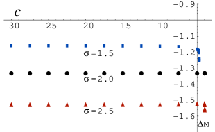
Figure 6: One-loop correction to the one-component topological kink (TK1) mass in units of $\hbar m$. $\bullet$, DHN formula . $\Box$, asymptotic series (left) The One-loop Quantum Mass Correction in the cases $\sigma=1.5$, $\sigma=2.0$ and $\sigma=2.5$ (right)

4.2 Semi-classical masses of kink families

We now try to compute the one-loop correction to the classical mass for the whole kink family

This task is easy if $\sigma=2$. Although the family of Schrödinger operators governing the small fluctuations around the TK2 kinks is non-diagonal,

$${\cal K}(b)=\left(\begin{array}[]{cc}-\frac{d^{2}}{dx^{2}}+6\frac{\sinh^{2}(2x)+b^{2}-1}{(\cosh(2x)+b)^{2}}-2&12\sqrt{b^{2}-1}\frac{\sinh(2x)}{(\cosh(2x)+b)^{2}}\\[5.69046pt] 12\sqrt{b^{2}-1}\frac{\sinh(2x)}{(\cosh(2x)+b)^{2}}&-\frac{d^{2}}{dx^{2}}+6\frac{\sinh^{2}(2x)+b^{2}-1}{(\cosh(2x)+b)^{2}}-2\end{array}\right)\qquad,$$

a rotation of $45^{0}$ in the internal space ${\mathbb{R}}^{2}$, $\vec{e}_{1}=\frac{1}{\sqrt{2}}(\vec{\varepsilon}_{1}+\vec{\varepsilon}_{2})$, $\vec{e}_{2}=\frac{1}{\sqrt{2}}(\vec{\varepsilon}_{1}-\vec{\varepsilon}_{2})$, shows that the system is uncoupled. Writing $\vec{\phi}=\psi_{1}\vec{\varepsilon}_{1}+\psi_{2}\vec{\varepsilon}_{2}$, we have that:

$$T_{\sigma=2}=\frac{1}{2}\left(\frac{d\psi_{1}}{dx}\right)^{2}+\frac{1}{2}\left(\frac{d\psi_{2}}{dx}\right)^{2}\qquad,\qquad U_{\sigma=2}=4\left(\psi_{1}^{2}-\frac{1}{8}\right)+4\left(\psi_{2}^{2}-\frac{1}{8}\right)$$

and the degenerate kink family is given as:

$$\vec{\phi}_{TK2^{*}}[x;a_{1},a_{2}]=\frac{(-1)^{\alpha}}{2\sqrt{2}}\tanh(x+a_{1})\vec{\varepsilon}_{1}+\frac{(-1)^{\beta}}{2\sqrt{2}}\tanh(x+a_{2})\vec{\varepsilon}_{2}\quad.$$

The alternative form of the Hessian is:

$${\cal K}(a_{1},a_{2})=\left(\begin{array}[]{cc}-\frac{d^{2}}{dx^{2}}+4-\frac{6}{\cosh^{2}(x+a_{1})}&0\\ 0&-\frac{d^{2}}{dx^{2}}+4-\frac{6}{\cosh^{2}(x+a_{2})}\end{array}\right)\qquad.$$

Therefore, $\Delta M(TK2^{*}[a_{1},a_{2}])=\hbar m(\frac{1}{\sqrt{3}}-\frac{6}{\pi})$. The kink degeneracy is not broken by quantum fluctuations at the one-loop level.

For generic $\sigma$ there are no analytical solutions available. We can however solve the first-order equations (4) by standard numerical methods and setting, for example, the “initial” conditions:

$$\phi_{1}(0)=0\qquad,\qquad\frac{\sigma}{2(1-\sigma)}\phi_{2}^{2}(0)-\frac{c}{2\sigma}|\phi_{2}(0)|^{\frac{2}{\sigma}}=\frac{1}{4}\qquad.$$

The polynomial kink solutions thus generated allow one to compute the coefficients $[a_{n}]_{aa}({\cal K})$. The results obtained via this numerical procedure are shown in Figure 6 (right). There is a breaking of the degeneracy for values of $c$ close to $c^{S}$ if $\sigma\neq 2$. The mass correction is lower when the two basic lumps are far apart; henceforth, repulsive forces are induced by the quantum fluctuations.

The $\sigma={1\over 2}$ case provides us with a qualitative understanding of what is going on. The plot of the diagonal components of the potential in the Schrödinger operator (10) for several values of $c$ shows that the potential in the second component starts to be repulsive at the value of $c$ where the two lumps start to split.

 

  

Figure 7: Diagonal components of the potential for c=-30, c=-1, c=0.1, c=0.245 and c=0.249.

References

• [1]
• [2] J.A. de Azcarraga, J.P. Gauntlett, J.M. Izquierdo and P.K. Townsend, Phys. Rev. Lett. 22 (1989) 2443. J.A. de Azcarraga, J.M. Izquierdo and P.K. Townsend, Phys. Rev. D45 (1992) R3321.
• [3] M. Cvetic, F. Quevedo and S.J. Rey, Phys. Rev. Lett. 67 (1991) 1836. M. Cvetic, S. Griffies and S. J. Rey, Nucl. Phys. B381 (1992) 301. M. Cvetic, S. Griffies and S.J. Rey, Nucl. Phys. B389 (1993) 3.
• [4] D. Bazeia, J.R.S. Nascimento, R. Ribeiro, and, D. J. Toledo, J. Phys. A30 (1997) 8157; D. Bazeia, M.J. Dos Santos and R. F. Ribeiro, Phys. Lett. A208 (1995) 84.
• [5] M. Shifman and M. Voloshin, Phys. Rev. D57 (1998) 2590.
• [6] A. Alonso Izquierdo, M.A. Gonzalez Leon and J. Mateos Guilarte, Phys. Rev. D65 (2002) 085012.
• [7] M. Eto and N. Sakai, β€œSolvable models of domain walls in ${\cal N}=1$ supergravity”, hep-th/0307276.
• [8] N. Sakai and R. Sugisaka, Phys. Rev. D66 (2002) 045010.
• [9] A. Alonso-Izquierdo, M. A. Gonzalez Leon, J. Mateos Guilarte and M. de la Torre Mayado, Phys. Rev. D66 (2002) 105022.
• [10] J. Gomis, Leuven Lectures on Branes, unpublished, 2003.
• [11] A. Alonso-Izquierdo, W. Garcia Fuertes, M.A. Gonzalez Leon and J. Mateos Guilarte, β€œOne-loop corrections to classical masses of kink families”, hep-th/0304125.
• [12] K. Fujikawa and P. van Nieuwenhuizen, β€œTopological anomalies from the path integral measure in superspace”, hep-th/0305144, to appear in Ann. Phys.
• [13] A. Alonso Izquierdo, M.A. Gonzalez Leon and J. Mateos Guilarte, Nonlinearity 15 (2002) 1097.
• [14] N. Manton, Phys. Lett. B110 (1982) 54.
• [15] M. Bordag, A. Goldhaber, P. van Nieuwenhuizen and D. Vassilevich, Phys. Rev. ${\bf D66}$ (2002) 125014.
• [16] A. Alonso-Izquierdo, W. Garcia Fuertes, M.A. Gonzalez Leon and J. Mateos Guilarte, Nucl. Phys. ${\bf B635}$ (2002) 525.
• [17] A. Alonso-Izquierdo, W. Garcia Fuertes, M.A. Gonzalez Leon and J. Mateos Guilarte, Nucl. Phys. ${\bf B638}$ (2002) 378.