Large scale correlations in normal non-Hermitian matrix ensembles

We compute the large scale (macroscopic) correlations in ensembles of normal random matrices with a general non-Gaussian measure and in ensembles of general non-Hermition matrices with a class of non-Gaussian measures. In both cases the eigenvalues are complex and in the large $N$ limit they occupy a domain in the complex plane. For the case when the support of eigenvalues is a connected compact domain, we compute two-, three- and four-point connected correlation functions in the first non-vanishing order in $1/N$ in a manner that the algorithm of computing higher correlations becomes clear. The correlation functions are expressed through the solution of the Dirichlet boundary problem in the domain complementary to the support of eigenvalues.

ITEP-TH-49/02

1 Introduction

A matrix $M$ is called normal if it commutes with its Hermitian conjugated: $[M,M^{{\dagger}}]=0$. The both matrices can be simultaneously diagonalized, the eigenvalues being complex numbers. The partition function of normal matrices has the general form

$$Z_{N}=\int_{\rm normal}d\mu(M)e^{\frac{1}{\hbar}{\rm tr}\,W(M,M^{{\dagger}})}.$$ (1)

Here $\hbar$ is a parameter, and the measure of integration over normal $N\times N$ matrices is induced from the flat metric on the space of all complex matrices. Like in other random matrix models, the large $N$ limit of interest implies $N\to\infty$, $\hbar\to 0$, while $N\hbar$ stays finite.

In a particular case, when Laplacian of the potential $W(z,\bar{z})$ is a constant in a big domain of a complex plane, i.e.,

$$W=-MM^{{\dagger}}+V(M)+\bar{V}(M^{{\dagger}}),$$ (2)

where $V(z)$ and $\bar{V}(z)$ are holomorphic functions, the normal matrix ensemble is equivalent to the ensemble of general complex matrices. It generalizes the Ginibre-Girko Gaussian ensemble [1]. In this, perhaps the most interesting case for applications, the model bears some formal similarities with the model of two Hermitian random matrices [2] and the matrix quantum mechanics in a singlet sector [3, 4]. Unlike models of few Hermitian matrices, the normal matrix model is integrable for a general class of potentials, not only of the form (2).

Applications and studies of matrix ensembles with complex eigenvalues are numerous. A large list of references can be found in recent papers [5]. New applications to diffusion limited growth models (Laplacian growth) [6], complex analysis [7]-[10] and Quantum Hall effect [11] were found recently.

Despite of a comprehensive literature on the model of one and two Hermitian matrices, interest to the normal matrix ensemble, first introduced in [12] and further studied in [13], as well as to a model of general complex matrices with potential (2), just starts to grow. In this paper we revisit the ensemble of normal random matrices to calculate the large $N$ limit of correlation functions under condition that separation between arguments is much more than an average distance between eigenvalues (macroscopic, or smoothed correlations). Short scale (microscopic) correlations in the ensemble with the potential (2) are well studied (see e.g. [15] for a review).

At large $N$ the eigenvalues of the random matrices are distributed within a domain (with sharp edges) of a complex plane with a density proportional to $\hbar^{-1}\Delta W$, where $\Delta$ is the 2D Laplace operator. We assume that the support of eigenvalues is a single connected bounded domain $D$, and that the boundary is a Jordan curve. Analytical properties of this curve determines the correlation functions.

We will show that correlation functions are expressed through the objects of the Dirichlet boundary problem of the domain complimentary to the support of eigenvalues. Namely, the two-point correlations are expressed through the Dirichlet Green function, while higher multi-point correlations are expressed through the Neumann jump on the boundary, through the Bergman kernel and through the curvature of the boundary. The objects similar to the correlation functions previously appeared in studies of thermal fluctuations in classical confined Coulomb plasma [14] (see also [15] for a review) and in recent studies of integrable structure of the Dirichlet boundary problem in [10]. If the potential $W$ is such that the support of eigenvalues collapses to a cut (or cuts), the normal matrix model reproduces known large $N$-limit features of the Hermitian matrix model.

We compute two-, three- and four-point connected functions of density of eigenvalues in the leading order in $N$, in a manner that the algorithm of computing higher correlation functions becomes clear. Connected density correlators are localized at the edge of the support of eigenvalues and show some universal features. They depend on the potential only through a shape of the support of the eigenvalues and boundary values of a finite number of derivatives of the potential. In the literature on Hermitian random matrices the universal character of correlations has been emphasized in Refs. [16, 17]. The two-point functions are distinguished since they depends on the support of the eigenvalues only. The two-point function has been previously computed in Refs. [14] in the course of studies of confined Coulomb plasma.

Other aspects, including integrable structure of the model (discussed already in [13, 18]), semiclassical properties of biorthogonal polynomials, critical points (a boundary with cusps), disconnected supports of eigenvalues, correlations at short distances, etc., will be addressed elsewhere.

2 Preliminaries

The measure of normal matrices.

The measure in (1) is induced from the flat metric $||\delta M||^{2}=\mbox{tr}\,(\delta M\delta M^{{\dagger}})$ in the space of all complex matrices. Formally, one can write $d\mu(M)=\delta([M,M^{{\dagger}}])dMdM^{{\dagger}}$, where the delta-function selects the subspace of normal matrices. To introduce coordinates in this subspace, one uses of the decomposition $M=UZU^{{\dagger}}$ , where $U$ is a unitary matrix and $Z=\mbox{diag}\,(z_{1},\ldots,z_{N})$ is a diagonal matrix of eigenvalues . The measure is then given by

$$d\mu(M)=\frac{d\mu_{0}(U)}{N!\,\mbox{Vol}\,({\cal U}(N))}|\Delta_{N}(z)|^{2}\prod_{i=1}^{N}d^{2}z_{i},$$ (3)

here $d^{2}z\equiv dxdy$ for $z=x+iy$, $d\mu_{0}$ is the Haar measure on the unitary group ${\cal U}(N)$, and $\Delta_{N}(z)=\det(z_{j}^{i-1})_{1\leq i,j\leq N}=\prod_{i>j}^{N}(z_{i}-z_{j})$ is the Vandermonde determinant.

If $A(M)$ is any invariant function (i.e., a symmetric function of eigenvalues) of a matrix $M$ (and $M^{{\dagger}}$), then the mean value

$$\left<A\right>=\frac{\int d\mu(M)A(M)e^{\frac{1}{\hbar}W}}{\int d\mu(M)e^{\frac{1}{\hbar}W}}$$ (4)

is expressed through the integral over eigenvalues

$$\left<A\right>=\frac{1}{N!Z_{N}}\int A(z)|\Delta_{N}(z)|^{2}\prod_{j=1}^{N}\left(e^{\frac{1}{\hbar}W(z_{j},\bar{z}_{j})}d^{2}z_{j}\right),$$ (5)

where the partition function is

$$Z_{N}=\frac{1}{N!}\int|\Delta_{N}(z)|^{2}\prod_{j=1}^{N}\left(e^{\frac{1}{\hbar}W(z_{j},\bar{z}_{j})}d^{2}z_{j}\right).$$ (6)

Potential.

For notational simplicity, we shall write simply $W(z)$ instead of $W(z,\bar{z})$. We assume that $W$ is a real-valued function with (at least local) minimum at the origin and set $W(0)=0$ for convenience. We also assume that the integral (6) converges and that $W$ is a regular function in both variables at the origin. We shall also set

$$\sigma(z)=-\frac{1}{\pi}\partial_{z}\partial_{\bar{z}}W(z)=-\frac{1}{4\pi}\Delta W,$$ (7)

and assume that $\sigma(z)>0$.

A special interesting case [11] occurs if the potential is harmonic in some big domain around the origin. Then in this domain $\sigma(z)=\mbox{constant}$, say, set to be $\pi^{-1}$, and

$$W=-|z|^{2}+V(z)+\bar{V}(\bar{z}),$$ (8)

where $V(z)$ is a holomorphic function.

The measure of complex matrices.

If the potential is chosen in the form (8), then the same measure, up to a numerical factor, appears in complex random matrices. In this case the relevant decomposition reads: $M=U(Z+R)U^{\dagger}$, where $U$, $Z$ are again unitary and diagonal matrix respectively, and $R$ is an upper triangular matrix. The measure (3) acquires a multiplicative factor $\prod_{ij}dR_{ij}e^{-R_{ij}^{2}}$ (we use the fact that $\mbox{tr}\,MM^{\dagger}=\mbox{tr}\,ZZ^{\dagger}+\mbox{tr}\,RR^{\dagger}$). As a result the representation (5) holds [19].

Coherent states of particles in magnetic field.

Most of the known matrix ensembles represent coherent states of $N$ fermions. Fermonic representations are well known in the case of Hermitian matrices (see, e.g., [20]), where fermions live on a line and are confined by a potential.

Complex matrix ensembles also enjoy a fermionic representation [21, 11]. In this case fermions are situated on a plane and occupy the lowest energy level of a strong magnetic field $B(z)$, the magnetic field is not necessarily uniform. It is related to the potential by $B(z)=2\pi\sigma(z)$. The coherent state of the fully occupied lowest level is

$$\Psi(z_{1},\dots,z_{N})=\frac{1}{\sqrt{N!}}\Delta_{N}(z)\,e^{\sum_{j=1}^{N}\frac{1}{2\hbar}W(z_{j})},\quad Z_{N}=\int|\Psi(z_{1},\dots,z_{N})|^{2}\prod d^{2}z_{i}.$$ (9)

So $Z_{N}$, in this picture, is the normalization factor of the wave function.

Example: Gaussian model.

In the case

$$W(z)=-\pi\sigma|z|^{2}+2{\cal R}e(t_{1}z+t_{2}z^{2})\,,\;\;\;\;\;\sigma>0\,,$$

(the Ginibre-Girko ensemble) the partition function can be found explicitly even for finite $N$ (see e.g. [21]):

$$Z_{N}(\sigma,t_{1},t_{2})=Z_{N}^{(0)}(\pi\sigma)^{\frac{1}{2}(N^{2}-N)}(\pi^{2}\sigma^{2}-4t_{2}\bar{t}_{2})^{-\frac{1}{2}N^{2}}\exp\left(\frac{N}{\hbar}\,\frac{t_{1}^{2}\bar{t}_{2}+\bar{t}_{1}^{2}t_{2}+\pi\sigma|t_{1}|^{2}}{\pi^{2}\sigma^{2}-4t_{2}\bar{t}_{2}}\right),$$ (10)

where $Z_{N}^{(0)}=\hbar^{\frac{1}{2}N(N+1)}\pi^{N}\prod_{j=1}^{N-1}j!$ is the partition function for $W=-|z|^{2}$. Correlation functions in this case are expressed through Hermite polynomials and are known explicitly for any $N$.

Correlation functions of traces.

In this paper, we are interested in correlation functions of products of $n$ traces, $\left<\prod_{i=1}^{n}\,\mbox{tr}\,f_{i}(M)\right>$. Clearly, they are expressed through $n$-point correlation functions of the density of eigenvalues,

$$\rho(z)=\hbar\sum_{i=1}^{N}\delta^{(2)}(z-z_{i}).$$

We obviously have:

$$\hbar^{n}\left<\prod_{i=1}^{n}\,\mbox{tr}\,f_{i}(M)\right>=\int\left<\rho(z_{1})\ldots\rho(z_{n})\right>f_{1}(z_{1})\ldots f_{n}(z_{n})\prod_{j=1}^{n}d^{2}z_{j}.$$ (11)

So, the density correlation functions carry the necessary information.

It is customary to deal with connected part of a correlation function. In case of the 2-point function it is

$$\left<\rho(z_{1})\rho(z_{2})\right>_{\rm conn}=\left<\rho(z_{1})\rho(z_{2})\right>-\left<\rho(z_{1})\right>\left<\rho(z_{2})\right>.$$

As $N\to\infty$, the $n$-point correlation function of densities is $O(1)$ while the connected part of the $n$-point function is $O(N^{2-2n})$.

The method of functional derivatives.

Correlation functions are the linear responses to a small variation of the potential. Variation of the partition function (6) over a general potential $W(z)$ inserts $\frac{1}{\hbar}\sum_{i}\delta^{(2)}(z-z_{i})$ into the integral. Then

$$\left<\rho(z)\right>=\hbar^{2}\,\frac{\delta\log Z_{N}}{\delta W(z)}\,,\;\;\;\;\left<\rho(z_{1})\rho(z_{2})\right>_{{\rm conn}}=\hbar^{2}\frac{\delta\left<\rho(z_{1})\right>}{\delta W(z_{2})}\,,$$ (12)

and, more generally,

$$\left<\rho(z_{1})\ldots\,\rho(z_{n})\right>_{{\rm conn}}=\hbar^{2n}\,\frac{\delta^{n}\log Z_{N}}{\delta W(z_{1})\ldots\delta W(z_{n})}.$$

We shall use this method in the following version. Set $\delta W(z)=\varepsilon g(z)$, where $g$ is an arbitrary smooth function on the plane and $\varepsilon\to 0$. Then, in the first order in $\varepsilon$,

$$\hbar^{2}\delta\left<\mbox{tr}\,f(M)\right>=\varepsilon\left<\mbox{tr}\,f(M)\,\mbox{tr}\,g(M)\right>_{{\rm conn}}.$$ (13)

It is often convenient to consider correlations of the potential

$$\varphi(z)=\int\log|z-z^{\prime}|^{2}\rho(z^{\prime})d^{2}z^{\prime}=\hbar\mbox{ tr}\left(\log(z-M)(\bar{z}-M^{\dagger})\right),$$ (14)

and of the current field

$$J(z)\equiv\partial\varphi(z)=\hbar\,\mbox{tr}\left(\frac{1}{z-M}\right),$$ (15)

rather than correlations of density. The potential is the Bose field or the loop field of a (collective) field theory of the matrix model (more accurately, $\varphi$ is a negative mode part of a Bose field). The field theory is proved to be successful approach to Hermitian matrix ensembles [22]. Elsewhere we will develop this approach for the non-Hermitian ensembles. The potential is harmonic outside the support of eigenvalues except at infinity where it behaves as $2N\hbar\log|z|$. The current is holomorphic outside the support of eigenvalues.

In order to obtain the correlations of the potentials, one has to vary the partition function by $W(z)\to W(z)+\varepsilon\log|z-\zeta|^{2}$ where $\zeta$ is a parameter. We denote this particular deformation of the potential by $\delta_{\zeta}$:

$$\delta_{\zeta}W(z)=\varepsilon\log|z-\zeta|^{2}.$$ (16)

Under this variation the correlation function changes by insertion of the field $\varphi(\zeta)$:

$$\hbar^{2}\delta_{\zeta}\left<A\right>=\varepsilon\left<A\,\varphi(\zeta)\right>_{{\rm conn}}.$$ (17)

This is the linear responce relation used in the Coulomb gas theory [15].

While varying the potential it is important to distinguish a harmonic variation of the potential $W(z,\bar{z})\to W(z,\bar{z})+V(z)+\bar{V}(\bar{z})$, where $V(z)$ is a holomorphic function. This variation does not change $\Delta W$. To implement a harmonic variation one may extend the potential by adding a harmonic function $W\to W+2{\cal R}e\,\sum_{k\geq 1}t_{k}z^{k}$ and apply the operator $D(z)=\sum_{k\geq 1}\frac{z^{-k}}{k}\partial_{t_{k}}$ used in Refrs. [7]-[10]. Then correlators of holomorphic parts of the potential $\phi(z)=\hbar\mbox{tr}\log(z-M)$ are

$$\begin{array}[]{l}\left<\phi(z)\right>=\hbar N\log z-\hbar^{2}{D}(z)\log Z_{N},\\ \\ \displaystyle{\left<\prod_{i=1}^{n}\phi(z_{i})\right>_{{\rm conn}}=(-1)^{n}\hbar^{2n}\prod_{i=1}^{n}{D}(z_{i})\log Z_{N}\,,\;\;\;\;n\geq 2}.\end{array}$$ (18)

Dirichlet boundary problem.

We list some elements of the external Dirichlet boundary problem, which are extensively used below. More details can be found in [23, 24].

Let $D$ be a closed connected domain of the complex plane bounded by a smooth curve. Given a real analytic function $f(z)$ in a vicinity of the boundary, we may restrict it to the boundary of $D$. The external Dirichlet problem is to find a harmonic function in the exterior of $D$, whose value on the boundary is $f(z)$. We call this harmonic function the harmonic extension of $f(z)$ to the exterior and denote it by $f^{H}(z)$. It is given by the

• Dirichlet formula:

  $$f^{H}(z)=-\frac{1}{2\pi}\oint\partial_{n^{\prime}}G(z,z^{\prime})f(z^{\prime})|dz^{\prime}|,$$

  where $\partial_{n^{\prime}}$ is the normal derivative at the boundary with respect to the second variable, with the normal vector being directed to the exterior of the domain $D$.

  The Green function $G(z,z^{\prime})$ for the exterior problem is a harmonic function everywhere outside $D$ including infinity except the point $z=z^{\prime}$, where it has a logarithmic singularity: $G(z,z^{\prime})\to\log|z-z^{\prime}|$ as $z\to z^{\prime}$. If $z^{\prime}\to\infty$, then $G(z,\infty)\to-\log|z|$. The Green function is symmetric in $z,z^{\prime}$ and vanishes on the boundary. In particular, the harmonic extension of $\log|z-\zeta|$ in $z$ is

  $$(\log|z-\zeta|)^{H}=\log|z-\zeta|-G(z,\zeta)+G(z,\infty).$$ (19)

  If the point $\zeta$ happens to be inside, $G(z,\zeta)$ in this formula is understood to be null.

• The Green function can be expressed through a conformal map $w(z)$ from ${\bf C}\setminus D$ (the exterior of $D$) onto the exterior of the unit disk:

  $$G(z,z^{\prime})=\log\left|\frac{w(z)-w(z^{\prime})}{1-\overline{w(z)}w(z^{\prime})}\right|.$$ (20)

  This formula does not depend on the normalization of the map. It is convenient to fix $w(z)$ by the condition that it sends infinity to infinity and the coefficient in front of the leading term as $z\to\infty$ is real positive.

• Neumann external jump is the difference between normal derivatives of a smooth function at the boundary and its harmonic extension. The Neumann external jump operator ${\sf R}$ acts as follows:

  $$f(z)\mapsto({\sf R}f)(z)=\partial_{n}^{-}(f(z)\!-\!f^{H}(z)),\quad\quad z\in\partial D.$$ (21)

  The upperscript indicates that the derivative is taken in the exterior of the boundary. As it follows from the Dirichlet formula, the Neumann jump is an integral operator on the boundary curve with the kernel given by normal derivative of the Green function in both arguments: $({\sf R}f)(z)=\partial_{n}f(z)+\frac{1}{2\pi}\oint\partial_{n}\partial_{n^{\prime}}G(z,z^{\prime})f(z^{\prime})|dz^{\prime}|$. In fact this integral is not yet well-defined since the kernel has a second order pole on the contour. The operations of taking normal derivative and contour integration do not commute. The above formula has to be understood as $\partial_{n}\oint\partial_{n^{\prime}}G(z,z^{\prime})f(z^{\prime})|dz^{\prime}|$ Alternatively the formula is understood as the principal value integral:

  $$({\sf R}f)(z)=\partial_{n}f(z)+\frac{1}{2\pi}\mbox{P.V.}\oint\partial_{n}\partial_{n^{\prime}}G(z,z^{\prime})(f(z)-f(z^{\prime}))|dz^{\prime}|.$$ (22)

• Hadamard formula describes deformation of the Dirichlet Green function under deformation of the domain.

  

  
  

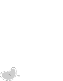
  Figure 1: The domain $D$ and vectors of normal displacement.

  A change of the boundary can be characterized by its normal displacement $\delta n(z)$, such that $\delta n(z)$ is a continuous function on the boundary (see Fig. 1). The Hadamard formula [25] expresses the deformation of the Green function through the Green function itself:

  $$\delta G(z_{1},z_{2})=\frac{1}{2\pi}\oint_{\partial D}\partial_{n}G(z_{1},\xi)\partial_{n}G(z_{2},\xi)\,\delta n(\xi)|d\xi|.$$ (23)

  A corollary of the Hadamard formula is the variation of the boundary value of a harmonic function under variation of the boundary. It reads

  $$\delta f^{H}(z)=({\sf R}f)(z)\,\delta n(z),\quad z\in\partial D.$$ (24)

3 Large $N$ limit

The large $N$ limit is understood as $N\to\infty$, $\hbar\to 0$ while $\hbar N$ is kept finite. The expansion in $N^{-1}$ is then equivalent to the expansion in $\hbar$. We call it a semiclassical limit.

Semiclassical density and the support of the eigenvalues.

To elaborate the semiclassical limit, we have to find the maximum of the integrand $|\Psi_{N}(z_{1},\dots,z_{N})|^{2}$ in (9). At finite $N$, it is given by the conditions $\partial{\log|\Psi_{N}|}/\partial z_{i}=0$ for every $i$:

$$\hbar\!\sum_{j=1,\neq i}^{N}\frac{1}{z_{i}-z_{j}}+\partial_{z_{i}}W(z_{i})=0,$$

or by the equation

$$\partial_{z}\left(\varphi_{0}(z)+W(z)\right)=\partial_{\bar{z}}\left(\varphi_{0}(z)+W(z)\right)=0\,,\quad\quad z\in D$$ (25)

in the limit. Here $\varphi_{0}(z)=\left<\varphi(z)\right>=\int\log|z-z^{\prime}|^{2}\left<\rho(z)\right>(z^{\prime})d^{2}z^{\prime}$ and $\left<\rho(z)\right>$ are expectation values of the potential and the density in the leading semiclassical approximation. The last equation holds inside the support of eigenvalues, $D$. It does not hold outside it. In the semiclassical approximation, $D$ is a domain with a well-defined sharp boundary determined by the potential $W$. An assumption that the support is a compact connected domain bounded by a Jordan curve implies restrictions on the potential. The restrictions do not reduce the number of parameters in the potential but rather ranges of their variation. We do not discuss them here. The assumption is valid, for example, for small perturbations of the Gaussian potential.

The solution for density is obtained by applying $\partial_{\bar{z}}$ to eq. (25):

$$\left<\rho(z)\right>=\left\{\begin{array}[]{ll}\sigma(z)&\quad\mbox{if}\quad z\in D\\ &\\ 0&\quad\mbox{ if}\quad z\in{\bf C}\setminus D.\end{array}\right.$$ (26)

The function $\sigma$ is introduced in (7). Consequently, $\displaystyle{\varphi_{0}(z)=}\int_{D}\log|z-z^{\prime}|^{2}\sigma(z^{\prime})d^{2}z^{\prime}$. This function is harmonic in the exterior of the domain except at infinity where it has a logarithmic singularity. Eq. (25) means that inside $D$, including the boundary, it is equal to $-W$ plus a constant. Since $W(0)=0$, the constant is $\displaystyle{\varphi_{0}(0)=\int_{D}\log|\xi|^{2}\sigma(\xi)d^{2}\xi}$, and so $\varphi_{0}(z)+W(z)=\varphi_{0}(0)$ for $z\in D$. Moreover, according to (25),

$$\partial_{n}\left(\varphi_{0}(z)+W(z)\right)=0,\quad\quad z\in\partial D,$$ (27)

so both tangential and normal derivatives of $\varphi_{0}+W$ at the boundary vanish.

Since $\varphi_{0}(z)-N\hbar\log|z|^{2}$ is harmonic outside, the harmonic extension of $W$ is

$$W^{H}(z)=\varphi_{0}(0)-\varphi_{0}(z)+N\hbar\left(\log|z|^{2}-\left(\log|z|^{2}\right)^{H}\right),$$ (28)

whence it follows that

$${\sf R}\left(W(z)+N\hbar\log|z|^{2}\right)=0\,.$$ (29)

This condition means, in other words, that the domain $D$ is such that the function $\partial_{z}W$ on its boundary is the boundary value of an analytic function in ${\bf C}\setminus D$. The latter, together with the normalization condition $\int_{D}\Delta Wd^{2}z=-4\pi\hbar N$, determines the shape of the support of eigenvalues.

For the potential of the form (8) with $V(z)=\sum_{k\geq 1}t_{k}z^{k}$ this condition is somewhat more explicit. In this case, the shape of the domain is determined, by the relations

$$-\frac{1}{\pi k}\int_{D}z^{-k}dz=t_{k}\,,\;\;\;\;\frac{1}{\pi}\int_{D}d^{2}z=\hbar N.$$

such that$\pi\hbar N$ is the area of $D$ and $-\pi kt_{k}$ are harmonic moments of the domain complementary to $D$. The problem is thus equivalent to the inverse problem of 2D potential theory.

Using the relation $W(z)=\varphi_{0}(0)-\varphi_{0}(z)$, it is easy to find the value of $\hbar^{2}\log|\Psi_{N}|^{2}$ at the saddle point, which we denote by $F_{0}$:

$$F_{0}=-\,\int_{D}\!\int_{D}\log\left|\frac{1}{z}-\frac{1}{z^{\prime}}\right|\sigma(z)\sigma(z^{\prime})d^{2}zd^{2}z^{\prime}.$$ (30)

The leading asymptote of the partition function as $\hbar\to 0$ is therefore $Z_{N}\simeq e^{F_{0}/\hbar^{2}}$. By inspection one can check that the average density (26) can be also obtained by variation of (30): $\left<\rho(z)\right>=\delta F_{0}/\delta W(z)$.

The function $F_{0}$ plays an important role in the complex analysis. It generates conformal maps from the exterior of $D$ onto the unit disk and gives a formal solution to the Dirichlet boundary problem. See Sec. 4 of [10] for details.

Variation of the support of eigenvalues.

Let us examine the change of the support of eigenvalues $D$ under a small change of the potential at fixed $N$. In general, we can write: $\int_{\delta D}f(z)d^{2}z=\oint_{\partial D}\delta n(z)f(z)|dz|$ for any function $f$, where $\delta D$ stands for a strip between the domains $D(W+\delta W)$ and $D(W)$ and $\delta n$ has the same meaning as in the previous section (Fig. 1).

The variation of the saddle point condition is most conveniently found from (27):

$$\delta(\partial_{n}(W+\varphi_{0}))=\delta n\,\partial_{n}^{2}(W+\varphi_{0})+\partial_{n}\delta(W+\varphi_{0})=0.$$

where $z$ is on the boundary. Since both tangential and normal derivatives of $W+\varphi_{0}$ vanish on the boundary, one writes $\partial_{n}^{2}(W+\varphi_{0})=\Delta(W+\varphi_{0})=\Delta W=-4\pi\sigma$. This gives the variation of the boundary:

$$\delta n(z)=\frac{1}{4\pi\sigma(z)}({\sf R}\,\delta W).$$ (31)

Here ${\sf R}\,\delta W=\partial_{n}(\delta W-(\delta W)^{H})$ is the external Neumann jump operator defined by (21). (We used the fact that $-\delta\varphi_{0}$ is, up to a constant, the harmonic extension of $\delta W$ to the exterior domain, as is seen from (28).) Note that if the variation of the potential is harmonic outside $D$ including infinity the domain does not change.

Let us check that our result meets the requirement that $N$ stays constant under a variation of the potential. Since

$$\oint\delta n(z)\sigma(z)|dz|=\frac{1}{4\pi}\oint\partial_{n}\delta W(z)|dz|=\frac{1}{4\pi}\int_{D}\Delta\delta W(z)d^{2}z$$

it is easy to see that

$$\delta\int\left<\rho(z)\right>d^{2}z=\oint\delta n(z)\sigma(z)|dz|+\int_{D}\delta\sigma(z)d^{2}z=0,$$

so that $N$ is kept constant under this variation.

Consider special variations of the potential of the form $\delta_{\zeta}W=\varepsilon\log|z-\zeta|^{2}$. Then one is able to express ${\sf R}\delta_{\zeta}W$ through the Dirichlet Green function (cf. (19)). It is convenient to introduce the modified Green function:

$${\cal G}(z,\zeta)=G(z,\zeta)-G(z,\infty)-G(\infty,\zeta)\,.$$ (32)

It is easy to see that

$$\delta_{\zeta}n(z)=\frac{1}{2\pi\sigma(z)}\partial_{n}{\cal G}(z,\zeta).$$

(The last term in ${\cal G}$ vanishes under the normal derivative. It is included for the symmetry and future convenience.)

Variation of the boundary under variation of the size of the matrix.

If one varies the size of the matrix, $N\to N+\delta N$, keeping the potential fixed, the support of eigenvalues also changes its shape. To find how it grows, we note that $\delta W=0$ means that $\delta\varphi_{0}(z)=\delta\varphi_{0}(0)$ for all $z\in D$. Plugging here the integral representation of $\varphi_{0}$, we conclude that $\oint\log|z^{-1}-\xi^{-1}|\delta n(\xi)\,\sigma(\xi)|d\xi|=0$ for all $z$ in $D$, with the variation of the normalization condition being $\hbar\delta N=\oint\delta n(z)\sigma(z)|dz|$. These conditions are met with

$$\delta n(z)=-\frac{\hbar\delta N}{2\pi\sigma(z)}\partial_{n}G(z,\infty),$$ (33)

where $G(z,\infty)=-\log|w(z)|$. This describes the interface dynamics in Laplacian growth models, known as Darcy’s law (cf. [6]).

4 Connected correlation functions in the first non-vanishing order in $\hbar$.

Connected two-point function.

In order to obtain the two-point function one has to vary the one point function $\left<\rho(z)\right>=\Theta(z;D)\,\sigma(z)$, where $\Theta(z;D)$ is the characteristic function of the domain $D$: $\Theta(z;D)=1$ for $z\in D$ and $\Theta(z;D)=0$ for $z\notin D$. The variation reads

$$\delta\left<\rho\right>=\delta\sigma\,\Theta(z;D)+\sigma\,\delta\Theta(z;D).$$ (34)

The second term is localized on the contour. Let $\delta(z;\partial D)$ be a $\delta$-function located on the boundary of $D$, defined by the condition that $\int f(z)\delta(z;\partial D)d^{2}z=\oint_{\partial D}f(z)|dz|$ for any smooth function $f$. It is clear that $\delta\Theta(z;D)=\delta n(z)\delta(z;\partial D)$. Using the relation (31) between a variation of the potential and deformation of the domain, we write:

$$4\pi\delta\left<\rho\right>=-\Delta\delta W\,\Theta(z;D)+({\sf R}\,\delta W)\,\delta(z;\partial D).$$

To keep track of the singular boundary terms, it is helpful to integrate the variation of density with some reasonable function $f$ on the plane. This is equivalent to calculating $\delta\left<\mbox{tr}\,f(M)\right>$ instead of $\delta\left<\rho\right>$. Setting $\delta W=\varepsilon g$ we have:

$$\frac{4\pi}{\varepsilon}\int\delta\left<\rho\right>fd^{2}z=-\int_{D}\Delta g\,fd^{2}z+\oint_{\partial D}f({\sf R}g)\,|dz|\,.$$

The result is symmetric with respect to $f\leftrightarrow g$. With a help of the Green formula, it can be expressed through the Bergmann kernel (22):

$$\begin{array}[]{c}\hbar^{-2}\displaystyle{\left<\mbox{tr}\,f(M)\,\mbox{tr}\,g(M)\right>_{{\rm conn}}}=\displaystyle{\frac{1}{\pi}{\cal R}e\int_{D}\partial_{z}f(z)\partial_{\bar{z}}g(z)d^{2}z\,\,+}\\ \\ +\,\displaystyle{\frac{1}{8\pi^{2}}\oint\!\oint f(z)\partial_{n}\partial_{n^{\prime}}G(z,z^{\prime})g(z^{\prime})|dz||dz^{\prime}|}.\end{array}$$ (35)

Choosing $f(z)=\log|z_{1}-z|^{2}$, $g(z)=\log|z_{2}-z|^{2}$, we find the pair correlation function of the Bose field $\varphi(z)$:

$$\frac{1}{2\hbar^{2}}\left<\varphi(z_{1})\varphi(z_{2})\right>_{{\rm conn}}\,={\cal G}(z_{1},z_{2})-\log\frac{|z_{1}-z_{2}|}{r},$$ (36)

where ${\cal G}$ is introduced in (32) and $\log r=\lim_{z\to\infty}(\log|z|+G(z,\infty))$ is Robin’s constant ($r$ is the exterior conformal radius of the domain $D$, see e.g. [26]). The function in the r.h.s. is harmonic outside the domain. If one of the points, say $z_{1}$, is located inside, one sets the corresponding Green functions in (32) to be zero. In particular, if both points are inside, the correlation function is just

$$\frac{1}{2\hbar^{2}}\left<\varphi(z_{1})\varphi(z_{2})\right>_{{\rm conn}}\,=-\,\log\frac{|z_{1}-z_{2}|}{r}.$$ (37)

This result is valid for well separated points ($|z_{1}-z_{2}|^{2}>>N\hbar/\sigma$).

Taking holomorphic or antiholomorphic derivatives of (36), we find pair correlations of currents:

$$\hbar^{-2}\left<J(z_{1})J(z_{2})\right>_{{\rm conn}}=-\frac{1}{(z_{1}-z_{2})^{2}}+2\partial_{z_{1}}\partial_{z_{2}}G(z_{1},z_{2}),$$ (38)

$$\hbar^{-2}\left<J(z_{1})\,\bar{J}(z_{2})\right>_{{\rm conn}}=-\pi\delta^{(2)}(z_{1}-z_{2})+2\partial_{z_{1}}\partial_{\bar{z}_{2}}G(z_{1},z_{2})$$ (39)

(here it is implied that both points are outside). These results resemble the two-point functions of the Hermitian 2-matrix model found in [2]; they were also obtained in [14] in the study of thermal fluctuations of a confined 2D Coulomb gas.

Outside the domain formulas (36), (38) describe correlations also at merging points away from the boundary. In particular, the mean square fluctuation of the current is

$$\hbar^{-2}\left<J^{2}(z)\right>_{{\rm conn}}=\frac{1}{6}\{w;z\}\,,\;\;\;\;\;z\in{\bf C}\setminus D.$$ (40)

Here

$$\{w;z\}=\frac{w^{\prime\prime\prime}(z)}{w^{\prime}(z)}-\frac{3}{2}\left(\frac{w^{\prime\prime}(z)}{w^{\prime}(z)}\right)^{2}=6\,\lim_{z^{\prime}\to z}\left(2\partial_{z}\partial_{z^{\prime}}G(z,z^{\prime})-\frac{1}{(z-z^{\prime})^{2}}\right)$$ (41)

is the Schwarzian derivative of the conformal map $w(z)$.

These formulas show that there are local correlations in the bulk as well as strong long range correlations at the edge. (See [27] for a similar result in the context of classical Coulomb systems). At the same time further variation of the pair density correlation function suggests that, starting from $n=3$, the connected $n$-point density correlations vanish in the bulk in all orders of $\hbar$ (in fact they are exponential in $1/\hbar$). All the leading contribution (of order $\hbar^{2n-2}$) comes from the boundary.

Note that the result (35) is universal in the sense that it depends on the potential only through the form of the domain $D$. The universality holds for any connected correlation function of two traces.

The kernel in the boundary term in (35) is the absolute value of the Bergman kernel [28] of the domain ${\bf C}\setminus D$ at the boundary. Presumably, this result can be generalized to the more complicated case of non-connected supports of eigenvalues, with the boundary term being expressed through the Bergman kernel of the Schottky double of the Riemann surface ${\bf C}\setminus D$. For the Hermitian one-matrix model, where the support of eigenvalues shrinks to a number of cuts on the real axis, a similar result was recently obtained in [29].

Connected three-point function.

The 3-point function can be obtained by further varying eq. (35). Let us first transform the r.h.s., to bring it to the form convenient for the varying. Using the Green formula, one rewrites the two point function as an integral over the entire complex plane plus the integral over the exterior of the domain

$$4\pi\hbar^{-2}\left<\mbox{tr}\,f(M)\,\mbox{tr}\,g(M)\right>_{{\rm conn}}=-\int_{{\bf C}}f\Delta gd^{2}z+\int_{{\bf C}\setminus D}(g-g^{H})\Delta fd^{2}z\,.$$

The variation of the first term is zero since it does not depend on the contour. The variation of the second term consists of two parts: the one coming from variation of the boundary and another one from variation of the integrand. The first part actually vanishes because the integrand equals zero on the boundary, where $g=g^{H}$. The variation of the integrand is $\displaystyle{-\int_{{\bf C}\setminus D}(\delta g^{H})\Delta f\,d^{2}z=\oint(\delta g^{H})({\sf R}f)|dz|}$ (where we substituted $f\to f-f^{H}$ under the Laplace operator and again used the Green formula). Next, we use the Hadamard formula (23) to compute the $\delta g^{H}$, the response of the harmonic extension of the function $g$ to a small change of the domain, taken on the boundary of the initial domain (24). The result is

$$4\pi\hbar^{-2}\delta\left<\mbox{tr}\,f(M)\,\mbox{tr}\,g(M)\right>_{{\rm conn}}=\oint({\sf R}\,f)({\sf R}\,g)\,\delta n|dz|.$$

Now, let us redefine $f=f_{1}$, $g=f_{2}$ and plug (31) for the $\delta n(z)$ with a function $f_{3}$: $\displaystyle{\delta n=\frac{\varepsilon}{4\pi\sigma}{\sf R}f_{3}}$. Using (17), we obtain the correlation function of three traces:

$$\left<\prod_{j=1}^{3}\mbox{tr}\,f_{j}(M)\right>_{{\rm conn}}=\frac{\hbar^{4}}{16\pi^{2}}\oint\frac{|dz|}{\sigma(z)}\prod_{j=1}^{3}\,{\sf R}f_{i}(z).$$ (42)

The answer is non-universal, i.e., it depends explicitly on the boundary value of the Laplacian of the potential. Note that if at least one of the functions $f_{j}$ is harmonic in ${\bf C}\setminus D$, then the correlation function vanishes (in this leading order in $\hbar$ of course).

Alternatively, one can apply the Hadamard formula directly to the 2-point correlation function of the potentials $\varphi$ (36). We have

$$\left<\varphi(z_{1})\varphi(z_{2})\varphi(z_{3})\right>_{{\rm conn}}=\frac{\hbar^{2}}{\varepsilon}\delta_{z_{3}}\left<\varphi(z_{1})\varphi(z_{2})\right>_{{\rm conn}}=2\frac{\hbar^{4}}{\varepsilon}\delta_{z_{3}}\left[{\cal G}(z_{1},z_{2})+\log r\right]\,=$$

$$=\frac{\hbar^{4}}{\varepsilon\pi}\oint\partial_{n}{\cal G}(z_{1},\xi)\partial_{n}{\cal G}(z_{2},\xi)\,\delta_{z_{3}}n(\xi)\,|d\xi|\,=$$

$$=\frac{\hbar^{4}}{2\pi^{2}}\oint\frac{|d\xi|}{\sigma(\xi)}\partial_{n}{\cal G}(z_{1},\xi)\partial_{n}{\cal G}(z_{2},\xi)\,\partial_{n}{\cal G}(z_{3},\xi)\,.$$

The result agrees with the formula for the third order derivatives of the tau-function obtained in [10] within a different approach (also based on the Hadamard variational formula).

For example, in the case $W=-|z|^{2}$, the support is a disk of the radius $R=\sqrt{\hbar N}$. The conformal map is simply $w(z)=z/R$ and the above formula gives

$$\left<\prod_{j=1}^{3}\varphi(\lambda_{j})\right>_{{\rm conn}}=-2\hbar R^{2}{\cal R}e\,\left(\frac{1}{(\lambda_{1}\bar{\lambda}_{2}-R^{2})(\lambda_{1}\bar{\lambda}_{3}-R^{2})}+\,[1\leftrightarrow 2],\ +\,[1\leftrightarrow 3]\,\right).$$

Finite $N$ formulas for the general $n$-point correlations reviewed in [15] should be able to be used to reclaim the same result.

Variation of contour integrals.

One may proceed in the same way to find the connected $n$-point correlation functions. Starting from $n=4$, however, one encounters technical difficulties.

When passing from 2-point to 3-point functions we transformed integral over the boundary into a bulk integral since the latter is easier to vary. Passing to 4-point functions, one needs to vary the contour integral in (42) which does not seem to be naturally representable in a bulk form. We have to learn how to vary contour integrals. Here are general rules.

Consider the contour integral of the general form $\oint F(f(z),\partial_{n}f(z))ds$ where $ds=|dz|$ is the line element along the boundary curve and $F$ is any fixed function. Calculating the linear response to the deformation of the contour, one should vary all items in the integral independently and add the results. There are four elements to be varied: the support of the integral $\oint$, the $\partial_{n}$, the line element $ds$ and the function $f$. By variation of the $\oint$ we mean integration of the old function over the new contour. This gives $\oint\delta n\,\partial_{n}F\,ds.$ The change of the slope of the normal vector results in $\delta\frac{\partial}{\partial n}=-\partial_{s}(\delta n)\frac{\partial}{\partial s}.$ The rescaling of the line element gives $\delta ds=\kappa\,\delta nds$, where $\kappa(z)$ is the local curvature of the boundary curve. The curvature is $\kappa=d\theta/ds$ where $\theta$ is the angle between the outward pointing normal vector to the curve and the $x$-axis. The formula $\kappa(z)=\partial_{n}\log\left|w(z)/w^{\prime}(z)\right|$ expresses the curvature through the conformal map. This formula is useful in calculating the 5-point function. We do not attempt to do this here. Another element is the Laplace operator on the boundary in terms of normal ($\partial_{n}$) and tangential ($\partial_{s}$) derivatives: $\Delta=\partial_{n}^{2}+\partial_{s}^{2}+\kappa\partial_{n}$.

At last, we have to vary the function $f$ if it explicitly depends on the contour. In particular, if this function is the harmonic extension of a contour-independent function on the plane, its variation on the boundary is given by (24).

Connected four-point function.

Let us elaborate the case $n=4$. In accordance with (17), we find $\left<\prod_{j=1}^{4}\mbox{tr}\,f_{j}(M)\right>_{{\rm conn}}$ from the response of the r.h.s. of eq. (42) to the variation of the potential $\delta W=\varepsilon f_{4}$, so that

$$\delta\sigma=-\frac{\varepsilon}{4\pi}\Delta f_{4}\,,\;\;\;\;\;\;\delta n=\frac{\varepsilon}{4\pi\sigma}{\sf R}f_{4}.$$ (43)

To get the result, we apply the above rules to the contour integral (42). Note that in this particular case a change of the slope of the normal vector gives no contribution since the functions under the normal derivative do not change along the boundary. Along this way we obtain the following result:

$$\begin{array}[]{c}\displaystyle{\frac{64\pi^{3}}{\hbar^{6}}\left<\prod_{j=1}^{4}\mbox{tr}\,f_{j}(M)\right>_{{\rm conn}}=\oint\frac{|dz|}{\sigma^{2}}\sum_{i=1}^{4}\Delta f_{i}\prod_{k=1,\neq i}^{4}{\sf R}f_{k}\,-}\\ \\ -\,\displaystyle{\oint\frac{|dz|}{\sigma^{2}}(\partial_{n}\log\sigma+2\kappa)\prod_{k=1}^{4}{\sf R}f_{k}\,-}\\ \\ -\,\displaystyle{\oint|dz|\left[\frac{{\sf R}f_{1}{\sf R}f_{2}}{\sigma}\,\partial_{n}\!\left(\frac{{\sf R}f_{3}{\sf R}f_{4}}{\sigma}\right)^{H}\,+[1\leftrightarrow 3]\,+\,[2\leftrightarrow 3]\,\right]}.\end{array}$$ (44)

The first two terms are explicitly symmetric with respect to all permutations of $(1,2,3,4)$. The third one is seemingly not, but in fact it is, as is clear from the Green formula.

In the 4-point correlation function the first term in the r.h.s. of (44) vanishes. For $\sigma(z)=1/\pi$, we get

$$\begin{array}[]{c}\displaystyle{\left<\prod_{j=1}^{4}\varphi(\lambda_{j})\right>_{{\rm conn}}=\frac{\hbar^{6}}{8\pi^{2}}\oint\!|dz|\!\,\partial_{n}\oint\!|dz^{\prime}|\,\partial_{n^{\prime}}{\cal G}(z,z^{\prime})\,\times}\\ \\ \times\,\,\displaystyle{\Bigl{(}\partial_{n}{\cal G}(\lambda_{1},z)\partial_{n}{\cal G}(\lambda_{2},z)\partial_{n^{\prime}}{\cal G}(\lambda_{3},z^{\prime})\partial_{n^{\prime}}{\cal G}(\lambda_{4},z^{\prime})+[1\leftrightarrow 3]+[2\leftrightarrow 3]\Bigr{)}}\,-\\ \\ \displaystyle{-\frac{\hbar^{6}}{2\pi}\oint|dz|\kappa(z)\prod_{j=1}^{4}\partial_{n}{\cal G}(\lambda_{j},z),}\end{array}$$ (45)

where ${\cal G}$ is defined by (32) and $\lambda_{j}$’s are assumed to be outside.

5 Discussion

We have shown that large scale properties of the normal matrix ensemble are obtained from the analytical properties of a curve on the complex plane. The curve bounds a semiclassical support of eigenvalues and is determined by the relation $\partial W(z)=-\hbar\left<\mbox{ tr}\frac{1}{z-M}\right>$.

Large scale correlation functions of the ensemble are objects of the Dirichlet boundary problem for the non-compact exterior domain complementary to the compact domain $D$. The two point function is essentially the Dirichlet Green function, the higher order functions are related to the deformation of the Green function under deformations of the curve. They are determined by successive applications of the Hadamard formula and are therefore expressed through the Neumann jump on the curve and through the Bergman kernel.

We expect that other objects of matrix ensembles, such as the genus ($1/N$) expansion of the partition function are recorded in the analytic properties of the curve. In particular, we expect that $F_{1}$ - a genus 1 correction to the partition function $\log Z_{N}$ (a correction of order $\hbar^{0}$) is related to the determinant of the Laplace operator in the exterior domain ${\bf C}\setminus D$.

References

- [1] J.Ginibre, J. Math. Phys. 6 (1965) 440, V.Girko Theor. Prob. Appl. 29 (1985), 694; ibid 30 (1986) 677
- [2] J.-M.Daul, V.Kazakov and I.Kostov, Nucl. Phys. B409 (1993) 311-338
- [3] S.Alexandrov, V.Kazakov and I.Kostov, to appear in Nucl. Phys. B, e-print archive: hep-th/0205079
- [4] B.Eynard, J. Phys. A 31 (1998) 8081, e-print archive: cond-mat/9801075
- [5] Y.Fyodorov, B.Khoruzhenko and H.-J.Sommers, Phys. Rev. Lett. 79 (1997) 557, e-print archive: cond-mat/9703152; J.Feinberg and A.Zee, Nucl. Phys. B504 (1997) 579-608, e-print archive: cond-mat/9703087; G.Akemann, e-print archive: hep-th/0204246
- [6] M.Mineev-Weinstein, P.B.Wiegmann and A.Zabrodin, Phys. Rev. Lett. 84 (2000) 5106-5109, e-print archive: nlin.SI/0001007
- [7] P.B.Wiegmann and A.Zabrodin, Commun. Math. Phys. 213 (2000) 523-538, e-print archive: hep-th/9909147;
- [8] I.Kostov, I.Krichever, M.Mineev-Weinstein, P.Wiegmann and A.Zabrodin, -function for analytic curves, Random matrices and their applications, MSRI publications, eds. P.Bleher and A.Its, vol.40, p. 285-299, Cambridge Academic Press, 2001, e-print archive: hep-th/0005259;
- [9] A.Zabrodin, Teor. Mat. Fiz. 129 (2001) 239-257 (in Russian, English translation: Theor. Math. Phys. 129 (2001) 1511-1525), e-print archive: math.CV/0104169
- [10] A.Marshakov, P.Wiegmann and A.Zabrodin, Commun. Math. Phys. 227 (2002) 131-153, e-print archive: hep-th/0109048
- [11] O.Agam, E.Bettelheim, P.Wiegmann and A.Zabrodin, Phys. Rev. Lett. 88 (2002) 236801, e-print archive: cond-mat/0111333
- [12] L.-L.Chau and Y.Yu, Phys. Lett. 167A (1992) 452
- [13] L.-L.Chau and O.Zaboronsky, Commun. Math. Phys. 196 (1998) 203-247, e-print archive: hep-th/9711091
- [14] A.Alastuey and B.Jancovici, J. Stat. Phys. 34 (1984) 557; B.Jancovici J. Stat. Phys. 80 (1995) 445
- [15] P.J.Forrester, Physics Reports, 301 (1998) 235-270
- [16] J.Ambjorn, J.Jurkiewicz and Y.Makeenko, Phys. Lett. B251 (1990) 517; J.Ambjorn, L.Chekhov, C.F.Kristjansen and Yu.Makeenko, Nucl. Phys. B404 (1993) 127-172; Erratum: ibid. B449 (1995) 681, e-print archive: hep-th/9302014
- [17] E.Brezin and A.Zee, Nucl. Phys. B402 (1993) 613
- [18] H.Aratyn, Lectures presented at the VIII J.A. Swieca Summer School, Section: Particles and Fields, Rio de Janeiro - Brasil - February/95, e-print archive: hep-th/9503211; M.Adler and P. van Moerbeke, Ann. of Math. (2) 149 (1999), no. 3, 921-976, e-print archive: hep-th/9907213
- [19] M.L.Mehta, Random matrices, Academic Press, NY, 1967
- [20] T.Banks, M.Douglas, N.Seiberg and S.Shenker, Phys. Lett. B238 (1990) 279
- [21] P.Di Francesco, M.Gaudin, C.Itzykson and F.Lesage, Int. J. Mod. Phys. A9 (1994) 4257-4351
- [22] S.Das and A.Jevicki, Mod. Phys. Lett. A5(1990) 1639
- [23] A. Hurwitz and R. Courant, Vorlesungen über allgemeine Funktionentheorie und elliptische Funktionen. Herausgegeben und ergänzt durch einen Abschnitt über geometrische Funktionentheorie, Springer-Verlag, 1964 (Russian translation, adapted by M.A. Evgrafov: Theory of functions, Nauka, Moscow, 1968)
- [24] G.Gakhov Boundary value problems, Dover, NY, 1990
- [25] J.Hadamard, Mem. presentes par divers savants a l’Acad. sci., 33 (1908).
- [26] E.Hille, Analytic function theory, v.II, Ginn and Company, 1962
- [27] B.Jancovici, J. Stat. Phys. 28 (1982) 43
- [28] S.Bergman, The kernel function and conformal mapping, Math. Surveys 5, AMS, Providence, 1950
- [29] Y.Chen and T.Grava, to appear in J. Phys. A, e-print archive: math-ph/0201024