Old Puzzles CERN-TH/2000-254

1 Introduction

We all know that matter such as the apple in figure 1 is made of molecules, molecules are made of atoms, and atoms are made of even smaller particles. It is a very old question what the most fundamental building blocks of matter are.

What we observe in the world is not only matter – there are also other things, shown in figure 1, such as light, and forces such as the electromagnetic or the gravitational force. All this is embedded in a three–dimensional space, and there is also one time dimension. It is another very old question where all this comes from.

Figure 1: What we observe

In my talk I first want to briefly review how far we have come in answering those old questions. I will begin with the things we know, which is the “Standard Model”, and then talk about the things that we can guess, which is superstring theory. After this review I will emphasise a key point at which our understanding of superstring theory presently stops: the problem of supersymmetry breaking and the cosmological constant. I will also explain in which direction I imagine a way out.

In a separate note [6] I will discuss my idea about what strings are made of.

2 The Standard Model

So what are the things we know? We know that the atoms that the apple is made of consist of electrons and nuclei, the nuclei are made of protons and neutrons, and protons and neutrons are made of three quarks each. The quarks come in three different states called “colors” – red, green and blue. Electrons and quarks are particles of spin ${1\over 2}$. There is another spin ${1\over 2}$ particle that is harder to detect, the neutrino. Together with the electron and two types of quarks, called $u$ and $d$, the neutrino forms a ‘family’ of quarks and leptons (figure 2). Alltogether we know three such families. So much for “matter”, i.e., for spin ${1\over 2}$ particles.

As for light, it is of course nothing but waves in the field of the electromagnetic force. Quantum field theory describes forces parallel to matter by elementary particles, but with integer spin. In the case of electromagnetism we have a spin 1 particle, the photon (figure 3).

Apart from the electromagnetic force there is also the “weak force”. The corresponding elementary particles of spin 1 are two W–bosons and one Z–bosons. Among other things, they can turn the electron and the neutrino into each other. More precisely, there is an $SU(2)$ symmetry associated with rotations in an internal complex two–dimensional vector space. The electron and the neutrino transform in the fundamental representation of this group and differ only by their orientation in this vector space; and the so-called ”gauge bosons” W and Z transform in the adjoint representation of this symmetry group.

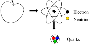
Figure 2: Particles with spin 1/2

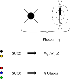
Figure 3: Particles with spin 1

There is also an $SU(3)$ symmetry associated with rotations in the 3–dimensional complex vector space generated by the colors of the quarks. The associated gauge bosons are 8 “gluons”. They mediate the strong interactions (the nuclear force) and are described by Quantum Chromodynamics (QCD). So alltogether, the known spin 1 particles are the gauge bosons associated with a symmetry group

$$SU(3)\times SU(2)\times U(1)\ .$$

All the spin ${1\over 2}$ and spin $1$ particles and their interactions mentioned are described in very good agreement with experiment by the Standard Model of Elementary Particle Physics, which also contains a spin 0 particle – the Higgs boson. The Higgs boson is held responsible for breaking the $SU(3)\times SU(2)\times U(1)$ symmetry group down to the observable $U(1)$ subgroup that corresponds to the electromagnetic force. It is the only particle that has not yet been observed directly in experiments.

There are of course many interesting aspects and details of the Standard Model which I will not go into since there are many other talks about them at this conference. Instead, let me move on to summarizing why we would like to go beyond the Standard Model.

3 Beyond the Standard Model

Why are we not yet happy with the Standard Model? First of all, there is of course the question why there should be so many different “elementary” particles, rather than only a single one. Second, the standard model contains 18 free parameters – the masses of these particles and the strenghts of their interactions – that are not predicted by the theory but are adjusted by hand to match the experimentally observed values. So clearly this is not yet a truly fundamental theory. And of course there are questions such as “why are there exactly three families of quarks and leptons?” and “why is the gauge group exactly $SU(3)\times SU(2)\times U(1)$?”

Before continuing the list of open questions, let me mention that there are ways to adress the issues mentioned so far. For example, one can assume that at very high energies, or equivalently at very small scales, there is a “Grand Unified Gauge Group” such as $SO(10)$ or $E_{6}$, that breaks down to the $SU(3)\times SU(2)\times U(1)$ subgroup that is observable at lower energies. This would unifiy the different gauge bosons in the sense that they would just form one representation of the grand unified group. Likewise, all the different spin ${1\over 2}$ particles in one family would just be different members of a single representation, or multiplet, of the large group.

One can also unify spin 1 particles and spin ${1\over 2}$ particles by introducing a symmetry that interchanges them, “supersymmetry”. With enough supersymmetry, the spin 0 Higgs boson can also be incorporated in such a “supermultiplet”.

One can even estimate the scales, at which such unifications might occur. The three gauge groups $U(1)$, $SU(2)$ and $SU(3)$ come with three coupling constants, $\alpha_{1},\alpha_{2}$ and $\alpha_{3}$. In field theory, such coupling constants are not really constant, but change with the scale, at which scattering experiments are performed. By extrapolating from their know values at large distance scales (low energy scales) down to small distance scales (high energy scales), one can see at what scales they meet.

In figure 4, the scales run from the size of the atom ($10^{-10}m$) through the size of the nucleus ($10^{-15}m$) and the scale of electroweak symmetry breaking (roughly $10^{-18}m$), which is about as far as we can see with accelerators, down to the the Planck scale (a fraction of $10^{-34}m$), where the strength of gravity becomes comparable with the strength of the other forces. Assuming that nothing else happens in between, the three coupling constants appear to unify at a scale (the “GUT scale”) that is not much larger than the Planck scale.

Actually, the three coupling constants do not meet exactly in the non–supersymmetric standard model. But if we assume that supersymmetry is restored at distance scales not much below the scale of electroweak symmetry breaking, then the couplings do meet within their error bars, at a scale only a few hundred times as large as the Planck scale. What we do not yet understand is the large “hierarchy” of 16 orders of magnitude between the Planck scale and the scale of electroweak symmetry breaking.

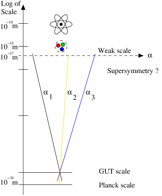
Figure 4: Scales and running coupling constants

While grand unification and supersymmetry may be promising first steps, they are not sufficient to adress two more fundamental shortcomings of the standard model. First of all, gravity doesn’t seem to fit into the framework. The gauge boson of gravity would be a spin 2 particle, the graviton, and there just isn’t a consistent quantum field theory of spin 2 particles, in the sense of a renormalizable, unitary continuum theory. In the context of gravity, another complete mystery that must be explained by a fundamental theory is why the cosmological constant is so small after supersymmetry breaking.

Second, questions such as “why is space–time four–dimensional?” cannot even be asked within the framework of the Standard Model, which is a priori formulated in four space–time dimensions.

4 Superstrings

If there is no field theory of pointlike gravitons, the next thing that one could try after points are lines (called strings), surfaces (called membranes), or higher-dimensional extended objects.

Let me first say why I will only talk about strings here. The reason is - and this has been understood only recently - that whatever theory of extended objects we start with, inasfar as the theory is consistent it is always just another formulation of string theory. E.g., there is the beginning of a theory of membranes, the 11–dimensional supermembrane theory. But it has been recognized that this membrane theory is in fact equivalent to string theory in the sense of strong–weak coupling duality. This is basically a much more elaborated version of the more familiar dualities of the two–dimensional Ising model (Kramers-Wannier duality) or of supersymmetric Yang-Mills theory (Olive-Montonen duality): the elementary excitations of the strong coupling limit (supermembranes) are solitons of the weak coupling limit (superstring theory), and vice versa.

So let us focus on string theory [1]. In string theory, all the different elementary particles including the graviton are assumed to be just different excitation modes of a single fundamental object, the superstring. It can indeed be shown that this leads to a consistent quantum theory that includes, in particular, the concepts of grand unification and supersymmetry. Superstring theory has only a single free parameter, the string tension ${1\over\alpha^{\prime}}$. And not even the space–time dimension is fixed in the theory, but is a property of its ground state.

Then why are we still not happy? Apart from the obvious question what strings are made of (we will come back to it later), the big problem with string theory is of course that it is so hard to test whether the theory is right or wrong. First of all, it seems unlikely that we will ever see the strings directly in experiments. It seems natural to assume that their size, the “string scale” (called ${\sqrt{\alpha^{\prime}}}$), is of the order of the Planck scale, and accelerators powerful enough to resolve such tiny scales would have to have galactic proportions.

One could still start from the hypothesis that the theory is correct, and try to “calculate it down” to low energies: what are its predictions for the number of families of quarks and leptons, for the gauge group, for particle masses, and for the space–time dimension? Do they agree with the Standard Model?

Let me indicate briefly how this is done by discussing scattering amplitudes. To simplify things I will pretend that spacetime has Euclidean signature. The scattering amplitudes can be translated to Minkowskian signature via a Wick rotation.

Computing scattering amplitudes in Euclidean string theory is very much like computing the energy of a soap film that is spanned, e.g., between the three boundaries in figure 5. The soap film represents the world–sheet that is swept out by the string as it moves through its embedding space, and the boundaries represent, in this case, one incoming and two outgoing strings. One first finds the minimal area surface that ends on the boundaries and computes its area $A$. The energy of the soap film is $A$ times the tension ${1\over\alpha^{\prime}}$. Very roughly, with Minkowskian signature and in the limit where the three strings at the boundaries become very small, the minimal area surface looks like an ordinary Feynman diagram of the Standard Model, such as that for the decay of a $W^{-}$ boson into an electron and an antineutrino. I am simplifying a little bit, but basically our soap film calculation should in this limit yield a string theory prediction for the decay rate and for the associated weak coupling constant.

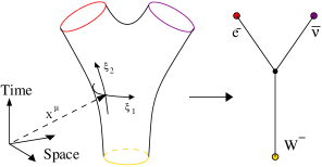
Figure 5: String world-sheets and soap films

As I said I am simplifying things. The soap film calculation is what one would do for classical strings, where the string world–sheet is a sharp surface – just like the world–line of a classical particle is a sharp line. In quantum mechanics, the string world–sheet fluctuates, though. To deal with this, one labels the world–sheet by coordinates $\xi_{1},\xi_{2}$. One then parametrizes the world–sheet by embedding coordinates $x^{\mu}(\xi)$, so that the space–time coordinates $x^{\mu}$ become two–dimensional fields that live on the world sheet. Quantum fluctuations of the world–sheet are taken into account by introducing a path integral over the coordinates and weighing it with $e$ to the minus the “soap film energy”. This yields $e$ to the minus the free energy $F$:

$$\exp\{-F\}\ =\ \int{\cal D}x^{\mu}(\xi)\ \exp\{-{1\over\alpha^{\prime}}A(x)\}\ .$$

Trying to do this path integral $\int{\cal D}x^{\mu}$ leads one into the fascinating area of two–dimensional conformal field theory. The two-dimensional fields are the coordinates $x^{\mu}(\xi)$, and $\alpha^{\prime}$ plays the role of $\hbar$.

I have no time to review two-dimensional field theory here, but I should take the time to point out right from the beginning its crucial limitation: two dimensional field theory can describe only perturbative string theory.

The diagrams in figure 5 are tree diagrams; they are computed from two-dimensional field theory on the shown genus zero surface with holes (the incoming or outgoing strings). g-Loop diagrams correspond to surfaces of genus $g$. They are suppressed by the $g$th power of the string coupling constant $\kappa^{2}$. Thus the loop expansion of particle theory becomes the genus expansion of two-dimensional field theory (figure 6).

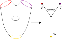
Figure 6: 1-loop scattering amplitudes from two-dimensional field theory on a torus

But what about nonperturbative effects that are invisible in the perturbation expansion in $\kappa$? Those cannot be seen in two-dimensional field theory on a surface of any genus. That this is a crucial limitation is clear from a comparison with QCD: just like important phenomena in QCD such as confinement and chiral symmetry breaking are invisible in its loop expansion, we must expect to miss crucial aspects of string theory in two-dimensional field theory. We will come back to this limitaion.

To conclude, there is a technical problem in calculating the string theory predictions for the “real world”, i.e. for the observable particle physics at low energy scales (up to TeV): our present technology allows us to only compute these predictions perturbatively in the string coupling constant $\kappa$. Although recently discovered strong-weak coupling dualities allow us to extend the range of validity from weak coupling to various strong coupling limits, the most interesting range of intermediate coupling is presently out of reach.

5 Perturbative string theory predictions

After these words of caution, let me move on to the results anyway – the perturbative string theory predictions for the observable world.

The good news is that gravity comes out right. One really recovers Einstein’s theory of general relativity as part of the low–energy limit, so this is a big success.

The bad news is that supersymmetry is unbroken in perturbative string theory. So Einstein’s gravity is really part of supergravity. This disagrees with the real world - we do not observe massless superpartners of the graviton. Moreover, it brings with it a long list of other problems. As is typical for supersymmetric theories, the ground state is degenerate. There are literally millions of distinct perturbative ground states with exactly the same energy (namely zero), and each of them makes a different prediction for the low-energy gauge group, the number of families, the number of scalar (Higgs) fields, etc.

Certainly the simplest ones of these ground states do not resemble the real world. Their gauge group comes out to be not $SU(3)\times SU(2)\times U(1)$, but either $SO(32)$ or $E_{8}\times E_{8}$. The number of families of quarks and leptons comes out to be not three but zero. But the most embarassing thing that comes out wrong is the number of space–time dimensions: it comes out to be 10!

Many - but not all - of the different ground states can be geometrically interpreted as compactifications of the simple 10-dimensional ones. When you roll up a sheet of paper, it looks one–dimensional rather than two–dimensional from the distance (figure 7). Likewise, six of the ten dimensions of string theory might be curled up into a tiny compact manifold (it turns out that it must be a Calabi–Yau manifold) such that the world looks 4–dimensional at scales much larger than the string scale. It can be seen that in this way one can also break the gauge group down to $SU(3)\times SU(2)\times U(1)$, and one can also obtain chiral families of quarks and leptons.

Figure 7: 4 dimensions from 10 dimensions

Millions of different ground states result because there are millions of topologically distinct ways to compactify six dimensions. In figure 7, just a few of these compactifications are plotted [2]. Each point represents one possible compactification. What is plotted is the number of Higgs fields (up to 480) that they predict against the number of families of chiral fermions that they predict (also up to 480!). Do we live on one of these points? Well, even if we did find a point that agrees with the observable world in terms of gauge group, number of Higgs fields and number of lepton families, we would not be convinced that string theory is correct. By picking a different point, we could “predict” pretty much any low energy physics we like – or in other words, we really cannot predict anything.

Figure 8: Some of the many string vacua

The reason for this lack of predictive power of perturbative string theory has already been mentioned: supersymmetry is unbroken perturbatively. Supersymmetry breaking must be a nonperturbative effect in string theory that is missed by the genus expansion of string amplitudes. Once supersymmetry is broken, the huge degeneracy of the string ground state can be expected to be lifted. So there should be a true vacuum of string theory after all, and it should lead to unique predictions.

The big obstacle to making contact between superstring theory and the real world is then to understand how supersymmetry is broken non-perturbatively.

6 The cosmological constant

The big clue to understanding supersymmetry breaking must be the cosmological constant: mysteriously, nature seems to manage to break supersymmetry without generating a huge cosmological constant. We first make a brief digression to recall what is so mysterious about this cosmological constant problem.

The energy density $\rho$ of the vacuum enters Einstein’s equations in the form of an effective cosmological constant $\lambda$:

$$R_{\mu\nu}-{1\over 2}g_{\mu\nu}R=\lambda g_{\mu\nu}\ \ \hbox{with}\ \ \lambda\ =8\pi G\rho\ ,$$ (1)

where $G$ is Newton’s constant. Such a cosmological constant $\lambda$ curves four–dimensional space–time, giving it a curvature radius $R_{curv}$ of order $\lambda^{-{1\over 2}}$. Only part of the curvature of the universe is due to the cosmological constant; other contributions come from visible and dark matter. This is accounted for by a factor $3\Omega_{\Lambda}$:

$$3\Omega_{\Lambda}\ R_{curv}^{-2}\ \sim\ \lambda\ .$$

$\Omega_{\Lambda}$ seems to have been measured to be $\Omega_{\Lambda}\sim{2\over 3}$ [3]. For a spacially flat universe, which is the case that seems to be realized in nature, this curvature radius implies an expanding universe with metric

$$ds^{2}\sim-dt^{2}+e^{Ht}d{\vec{x}}^{2}\ \ \hbox{with}\ \ 3\Omega_{\Lambda}H^{2}\sim\lambda.$$ (2)

The Hubble constant $H$ in our universe is of order

$$H\ \sim\ 10^{-33}eV\ \sim\ (10^{26}m)^{-1}\ .$$

The cosmological constant problem is the question why this is so small, given that we expect much larger contributions to the energy density of the vacuum from Standard Model physics. Let us briefly summarize why we expect such contributions.

First of all, there are classical effects. E.g., in the course of electroweak symmetry breaking the Higgs field is supposed to roll down its potential, thereby changing the vacuum energy density by an amount of order $(TeV)^{4}$. This would give a curvature radius of the universe in the millimeter range, which is not what we observe. Of course, the Higgs potential could be shifted such that its Minimum is at zero. Equivalently, a bare cosmological constant could be added in (1) that exactly cancels the cosmological constant induced by $\rho$. But this is just the fine–tuning problem: why should the bare cosmological constant be fine–tuned to exactly cancel the contributions from later phase transitions?

Even if we do find a reason why the minimum of the Higgs potential should be zero, the problem does not go away. There are other condensates in the Standard Model, such as the chiral and gluon condensates in QCD after chiral symmetry breaking. They should contribute an amount of order $(\Lambda_{QCD})^{4}$ to the cosmological constant, which would translate into a curvature radius of the universe in the kilometer range.

And even if one did not believe in chiral and gluon condensates, there would still remain what is perhaps the most mysterious aspect of the problem: the cosmological constant does not seem to receive contributions from the zero–point energy of the Standard Model fields. A harmonic oscillator has a ground state energy ${1\over 2}\hbar\omega$. In a field theory we have one oscillator for each momentum $k$ with frequency

$$\omega\ =\ \sqrt{k^{2}+m^{2}}\ .$$

In the case of the photon (with $m=0$), integrating over $k$ gives, for each of the two polarizations, a divergent contribution

$$\lambda\ \ =\ 8\pi G\ \int_{|k|\leq\Lambda}{d^{3}k\over(2\pi)^{3}}{1\over 2}\hbar\omega\ \sim\ {1\over 2\pi}{\Lambda^{4}\over m_{Pl}^{2}}$$ (3)

to the cosmological constant, where $\hbar G\ =\ m_{Pl}^{-2}$ and $\Lambda$ is a large–momentum cutoff. How large does this cutoff $\Lambda$ have to be? (3,2) tell us that $\Lambda$ is, on a logarithmic scale, half–way between the Planck mass and the Hubble constant.

$${H\over\Lambda}\ \ \ \sim\ \ \ {\Lambda\over m_{Pl}}.$$ (4)

It is straightforward to calculate that $\Lambda$ is several milli-eV, corresponding to a Compton wave length in the micrometer range. This is even larger than the wave–length of visible light: we can see with our bare eyes that there is no such cutoff in nature!

What can explain a zero cosmological constant is supersymmetry. In supersymmetric theories, the contributions from bosons and fermions to $\lambda$ have opposite signs and cancel. But in order to explain the smallness of the Hubble constant, supersymmetry would have to remain unbroken at least up to scales of the order of the above cutoff $\Lambda$, i.e. up to milli-eV scales (see figure 1).

In other words, the cosmological constant that seems to have been observed could be produced by a supermultiplet of particles with mass splittings of order milli-$eV$ (at least if the supertrace of the mass matrix of the supermultiplet vanishes). But unbroken supersymmetry up to milli-eV scales is of course ruled out for the Standard model: there is no superpartner of the photon with mass in the milli-eV range. If there was, the energy levels in atoms would be very different (if atoms were stable at all). So this is the dilemma.

7 Do we live on a soliton?

We should probably be grateful for this dilemma. The miracle of the nearly vanishing cosmological constant should be a crucial hint as to how nature breaks supersymmetry. Let me now tell you what I personally think that the smallness of the cosmological constant hints at: that we live on a non-supersymmetric soliton of superstring theory.

You might be familiar with extended solitons in solid state physics such as vortex lines in superconductors. 10-dimensional string theory also contains a variety of extended solitonic objects, so–called $p$–branes. A $p$–brane has $p$ space– and one time dimension. There are i.p. 3–branes (figure 8). Each point on it is surrounded by an $(n-1)$–sphere, if there are $n$ dimensions transverse to the brane (in our case, $n=6$, but it is useful to consider the more general case). It can be shown that there are gauge fields $A^{\mu}$, chiral fermions $\psi$ and scalar fields $\phi$ that live only on the 3–brane. These fields might make up the particles of the standard model, if we identify the 3–brane with the observable universe. Gravity, however, is not restricted to the brane in these models. Instead it lives all over the $(4+n)$–dimensional bulk.

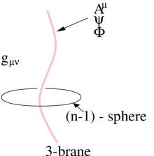
Figure 9: 3-branes embedded in $4+n$ dimensions.

Imagine now that we live on a stable non-supersymmetric soliton - a 3+1 dimensional brane inside the 10-dimensional space of superstring theory; so supersymmetry is broken only because of this brane. Why might this help solve the cosmological constant problem?

I will sketch the ideas of [4]. As we noted before, at least if the recent measurements of the cosmological constant can be trusted, the size of the cosmological constant is such that it could be produced by a supermultiplet of particles with supersymmetry being broken in the milli–$eV$ range. Whatever these particles are, they must be fundamentally different from the Standard Model particles, because they contribute to the cosmological constant, while the Standard Model particles obviously don’t.

The non–supersymmetric brane world scenario provides precisely such a fundamental difference between the Standard Model particles, which live on the brane, and other particles (the supergravity particles), which live in the bulk. So the idea is that the cosmological constant is produced only by the supergravity multiplet.

But why should the Standard Model particles not contribute to the cosmological constant at all? Well, the scenario does in fact provide a mechanism which could at least in principle do the job of soaking up the Standard Model vacuum energy: if the Standard Model is confined to a brane, then it is conceivable that the resulting brane cosmological constant only curves the space transverse to the brane, but not the space parallel to the brane [5] – so the curvature radius of the four-dimensional universe could still be huge.

It is very nontrivial and striking that the supersymmetry breaking scale $\Lambda$ of order milli–$eV$ in the gravity sector comes out naturally, if one assumes Standard Model supersymmetry breaking in the $TeV$ range (as required for the running coupling constants to meet, as mentioned earlier). One then expects e.g. a gravitino mass of order

$$m_{3/2}\ \sim\ {{(TeV)^{2}\over m_{Pl}}}\ \sim\ \Lambda\ \sim\ \hbox{milli-}eV\ .$$

Together with (4), one in fact predicts a relation between four vastly different scales in physics [4]: the Planck scale, the scale of supersymmetry breaking in the Standard Model, the inverse gravitino mass and the inverse Hubble expansion rate of the universe, whose square is of the same order $(10^{-33}eV)^{2}$ as the value of the cosmological constant that seems to have been recently observed [3]. This predicted relation is plotted in figure 9, which extends figure 4 up to cosmic scales. The solid horizontal lines are predicted to be equally spaced on a logarithmic scale, with step size roughly 15.5.

Figure 10: Predicted ratio of scales (to convert electron volt into meters: $(1eV)^{-1}\sim 2\cdot 10^{-7}m$.)

While there are certainly unresolved issues in this scenario (see, e.g., second reference in [4]), at least to the author it feels like pieces of a puzzle beginning to fall into place. But perhaps the best feature of this scenario is that it can be tested experimentally: it predicts gravitinos and other superpartners of the graviton with masses in the $milli-eV$ range. The precise masses of the superpartners of the graviton depend on the detailed non-BPS soliton solution, so the spectrum of supergravity masses should in principle be a window through which we can probe what kinds of branes our string compactification contains.

Masses in the $milli-eV$ range translate into a hypothetical gravitino or dilaton with Compton wavelength in the micrometer range. This is just at the border of not yet being ruled out by experiment, and it could be checked by short-distance measurements of gravity in the not-so-far future.

8 Conclusion

To summarize, the observation of apples, light and electromagnetic forces leads us to the Standard Model. The observation of gravity leads us to superstrings.

To compute the low-energy predictions of superstring theory and compare them with observation, a crucial step is to understand how supersymmetry is broken in string theory.

The crucial hint should be the smallness of the cosmological constant: its observed size is precisely such that it could be produced by the vacuum energy of the supergravity sector, if the observable universe was a four-dimensional non-supersymmetric soliton inside the ten-dimensional space-time of superstring theory.

This scenario predicts gravitinos and other superpartners of the graviton with masses in the milli-$eV$ range. They could be observed experimentally through short-distance measurements of gravity in the micrometer range.

References

- [1] Standard introductions to superstring theory: M. B. Green, J. H. Schwarz and E. Witten, “Superstring Theory.” Cambridge University Press ( 1987); J.Polchinski, ”String Theory”, Vol. 1 and 2, Cambridge University Press (1998); B. R. Greene, “The Elegant Universe,” New York, Norton (1999) 448 p.
- [2] A. Klemm and R. Schimmrigk, “Landau-Ginzburg string vacua,” Nucl. Phys. B411 (1994) 559.
- [3] N. Bahcall, J. P. Ostriker, S. Perlmutter and P. J. Steinhardt, “The Cosmic Triangle: Revealing the State of the Universe,” Science 284, 1481 (1999).
- [4] C. Schmidhuber, “Micrometer gravitinos and the cosmological constant,” Nucl. Phys. B585, 385 (2000). “Brane Supersymmetry Breaking and the Cosmological Constant: Open Problems,” Nucl. Phys. B619, 603 (2001).
- [5] V. A. Rubakov and M. E. Shaposhnikov, “Extra Space-Time Dimensions: Towards A Solution To The Cosmological Constant Problem,” Phys. Lett. B125, 139 (1983).
- [6] C. Schmidhuber, “Logical Quantum Field Theory,” in preparation.