UTTG-08-02

hep-th/0207114


All Genus Topological String Amplitudes and 5-brane Webs as Feynman Diagrams
Amer Iqbal


Theory Group, Department of Physics

University of Texas at Austin,

Austin, TX 78712, U.S.A.

A conjecture for computing all genus topological closed string amplitudes on toric local Calabi-Yau threefolds, by interpreting the associated 5-brane web as a Feynman diagram, is given. A propagator and three point vertex is defined which allows us to write down the amplitude associated with 5-brane web. We verify the conjecture that this amplitude is equal to the closed string partition function by computing integer invariants for resolved conifold and certain curves of low degree in local del Pezzo surfaces, local Hirzebruch surfaces and their various blowups.

1 Introduction

Topological string amplitudes have been of interest to physicists and mathematicians for a long time. For physicists these amplitudes compute terms in the low energy effective action of the theory obtained by compactifying IIA sting theory on a Calabi-Yau threefold [1]. They are of interest to mathematicians since they are the generating functions of Gromov-Witten invariants [2, 3] of holomorphic curves in Calabi-Yau threefold [4].

For the case of toric Calabi-Yau threefolds various techniques are available for computing these amplitudes. Localization can be used for a direct calculations in the A-model [5]. This was discussed in detail in [6] for genus zero case using mirror symmetry. Higher genus calculations, using localization, for the local IP2IsuperscriptP2\mbox{I}\!\mbox{P}^{2} case were carried out in [7]. B-model calculation, although tedious, provide another way of calculating these amplitudes up to certain unknown constants which can sometimes be fixed from their behavior at the singular points [8] in the moduli space and using the hidden integrality properties of the invariants [9].

Integer invariants of holomorphic curves in Calabi-Yau threefolds were defined in [10] and it was shown that topological closed string amplitudes when interpreted from the target space point of view are the generating functions of these integer invariants,

F(ω)=g=0gs2g2Fg(ω)=m=1βH2(X,𝖹𝖹)r=0Nβrm(2sin(mgs2))2r2emβω.𝐹𝜔superscriptsubscript𝑔0superscriptsubscript𝑔𝑠2𝑔2subscript𝐹𝑔𝜔superscriptsubscript𝑚1subscript𝛽subscript𝐻2𝑋𝖹𝖹superscriptsubscript𝑟0subscriptsuperscript𝑁𝑟𝛽𝑚superscript2sin𝑚subscript𝑔𝑠22𝑟2superscript𝑒𝑚𝛽𝜔\displaystyle F(\omega)=\sum_{g=0}^{\infty}g_{s}^{2g-2}F_{g}(\omega)=\sum_{m=1}^{\infty}\sum_{\beta\in H_{2}(X,{\sf Z\!\!\!Z})}\sum_{r=0}^{\infty}\frac{N^{r}_{\beta}}{m}(2\mbox{sin}(m\frac{g_{s}}{2}))^{2r-2}\,e^{-m\beta\cdot\omega}\,. (1)

Where X𝑋X is the Calabi-Yau with Kähler form ω𝜔\omega and Nβr𝖹𝖹subscriptsuperscript𝑁𝑟𝛽𝖹𝖹N^{r}_{\beta}\in{\sf Z\!\!\!Z} are the invariants. Topological open string amplitudes were reformulated in terms of open string integer invariants in [11] by interpreting them from the target space point of view.

A completely new way of obtaining the topological closed string amplitudes from the Chern-Simons theory was developed in [12] using geometric transition: deformation versus resolution of the singularity. The case of blown up conifold was discussed in detail and all genus closed string amplitude of the blown up conifold was derived from the partition function of the Chern-Simons theory on S3superscript𝑆3S^{3}. Recently this open-closed duality, Chern-Simons theory being the theory of topological open strings, was proved from the world-sheet point of view [13]. The fact that both open and closed string invariants are related to knot invariants in a geometry obtained via geometric transition has been checked for many cases [14, 15, 16, 17, 19, 20].

Closed string invariants for more complicated geometries, such as local toric del Pezzo surfaces, have been calculated from the Chern-Simons theory using geometric transition [20, 21]. Unlike the case of the resolved conifold, in these cases the Chern-Simons theory on the space obtained after geometric transition gets corrections from the holomorphic curves with boundaries on the 3-cycles [22]. This open-closed duality, Chern-Simons theory being the theory of open strings [22], has been checked in many cases and is by far the easiest method for calculating the Gromov-Witten invariants and check their hidden integrality properties as formulated in terms of integer invariants [10]

It is well known that knot invariants in the Chern-Simons theory can be calculated using the WZW theory. In this note we conjecture that using the 5-brane web description of toric local Calabi-Yau threefolds [23] the topological closed string partition function can be written directly using the propagator and vertex defined by states and operators in the large N𝑁N WZW theory. Since the 5-brane web naturally gives rise to a Riemann surface the topological closed string partition function is an amplitude associated with this Riemann surface. The conjecture is motivated by the lattice model interpretation of the topological closed string amplitudes given in [21]. It follows from their discussion once we recognize that the “three point vertex” is more basic than the four point vertex of the lattice model [21] and that all 5-brane web diagrams can be constructed from (1,0) 5-brane (“the propagator”) , three point vertex given by (1,0), (0,1) (1,1) 5-branes and their SL(2,𝖹𝖹)𝑆𝐿2𝖹𝖹SL(2,{\sf Z\!\!\!Z}) transforms. We verify the idea by computing integer invariants, from this 5-brane web amplitude, for various geometries.

Using the 5-brane/7-brane description of certain local Calabi-Yau threefolds, developed in [24] we conjecture the form of closed string partition function for some non-toric threefolds. From the 5-brane/7-brane description of toric local Calabi-Yau threefolds it appears that closed string partition function is given by particular Feynman diagrams in the vacuum to vacuum amplitude. The case of non-toric threefolds will be discussed in more detail elsewhere[18].

This paper is organized as follows. In section two we discuss briefly the 5-brane web description of toric local Calabi-Yau threefolds. We also discuss, in this section, the Riemann surface coming from the 5-brane web when IIB string theory is lifted to M-theory after compactification on a circle. In section two we define the propagator and the three point vertex using the states and the operators of the WZW theory. We also discuss the matrix elements and and their computation which will be needed later to work out the integer invariants. The matrix elements we will need are related to the Hopf link with linking number plus one and therefore the discussion of matrix elements is mostly based on section three of [21]. In section three we compute integer invariants for a few curves of low degree in various toric local Calabi-Yau threefolds with a single compact divisor from the 5-brane web description. A more complete account of these invariants for curves of higher degree in these geometries will be given elsewhere [18].

2 Local threefolds and 5-brane webs and the Riemann surface

In this section we discuss toric local Calabi-Yau threefolds, their dual description involving (p,q)𝑝𝑞(p,q) 5-branes of type IIB string theory and the Riemann surface associated with the web.

2.1 CY and 5-brane web

The relation between local toric Calabi-Yau spaces and 5-brane webs of type IIB string theory follows from the basic duality between M-theory on T2superscript𝑇2T^{2} and type IIB string theory on S1superscript𝑆1S^{1}. Consider as an example the resolved conifold which has a toric description given by the following equation [31],

|X1|2+|X2|2|X3|2|X4|2=r,superscriptsubscript𝑋12superscriptsubscript𝑋22superscriptsubscript𝑋32superscriptsubscript𝑋42𝑟\displaystyle|X_{1}|^{2}+|X_{2}|^{2}-|X_{3}|^{2}-|X_{4}|^{2}=r, (2)
(X1,X2,X3,X4)=(eiθX1,eiθX2,eiθX3,eiθX4).subscript𝑋1subscript𝑋2subscript𝑋3subscript𝑋4superscript𝑒𝑖𝜃subscript𝑋1superscript𝑒𝑖𝜃subscript𝑋2superscript𝑒𝑖𝜃subscript𝑋3superscript𝑒𝑖𝜃subscript𝑋4\displaystyle(X_{1},X_{2},X_{3},X_{4})=(e^{i\theta}\,X_{1},e^{i\theta}\,X_{2},e^{-i\theta}\,X_{3},e^{-i\theta}\,X_{4})\,.
Refer to caption
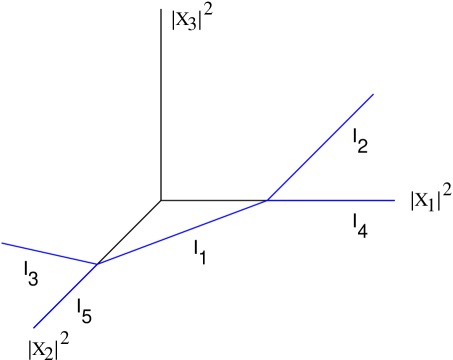
Figure 1: The resolved conifold. Line segments Iasubscript𝐼𝑎I_{a} represent different collapsing U(1)𝑈1U(1)’s.

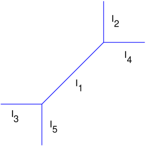
At a point, where none of Xisubscript𝑋𝑖X_{i} are zero we have a T4/U(1)superscript𝑇4𝑈1T^{4}/U(1). Where the U(1)𝑈1U(1) acts with charges (1,1,11)1111(1,1,-1-1) on the phases of Xasubscript𝑋𝑎X_{a} which form the T4superscript𝑇4T^{4}. On different line segments Iasubscript𝐼𝑎I_{a}, shown in Fig. 1, two different Xasubscript𝑋𝑎X_{a} become zero and therefore we are left with a single U(1)𝑈1U(1) after modding out. If we consider the R2superscriptR2\mbox{R}^{2} orthogonal to the line passing through the origin and making equal angle with all three axis then we get a T2superscript𝑇2T^{2} fibration over this plane with T2superscript𝑇2T^{2} degenerating as shown in Fig. 2.

Refer to caption
Figure 2: Projection of the resolved conifold.

On this plane we can choose the directions such that (p,q)𝑝𝑞(p,q) cycle degenerates along a line segment oriented in the (p,q)𝑝𝑞(p,q) direction. Now if we apply M-theory/IIB duality adiabatically we see that the T2superscript𝑇2T^{2} disappears and its information is encoded in the branes present along the locus of degeneration. The line segment directed in the (p,q)𝑝𝑞(p,q) direction , along which (p,q)𝑝𝑞(p,q) cycle was degenerating, now has (p,q)𝑝𝑞(p,q) 5-brane of IIB string theory.

The 5D 𝒩=1𝒩1{\cal N}=1 theory on the transverse space coming from M-theory on the CY is dual to the 5D 𝒩=1𝒩1{\cal N}=1 theory on the 5-brane web. By compactifying one direction transverse to the conifold we can go to type IIA string theory on the blown up conifold. Compactifying one of the common directions of the 5-branes we can go back to M-theory with 5-brane web becoming a single M5-brane wrapped on a Riemann surface embedded in R2×T2superscriptR2superscript𝑇2\mbox{R}^{2}\times T^{2}. We will see that this Riemann surface plays the central role in writing down the string partition function. This perhaps is related to the results of [27, 28] where relation between string partition functions and M5-brane theory was explored. The Riemann surface projects to R2superscriptR2\mbox{R}^{2} as a thickened 5-brane web. The 𝒩=2𝒩2{\cal N}=2 theory on the transverse space obtained by compactifying type IIA string theory on a local Calabi-Yau threefolds has a dual description as the theory on an M5-brane wrapped on the Riemann surface associated with the corresponding web.

Refer to caption
Figure 3: The Riemann surface associated with the 5-brane web dual to the resolved conifold.

For toric local Calabi-Yau this Riemann surface can easily be obtained from the toric data and plays an important role in constructing the mirror Calabi-Yau threefold. If the Riemann surface associated with web is given by f(eu,ev)=0𝑓superscript𝑒𝑢superscript𝑒𝑣0f(e^{u},e^{v})=0 (u,v being coordinates on R2×T2superscript𝑅2superscript𝑇2R^{2}\times T^{2}) then the mirror Calabi-Yau threefold is given by

f(eu,ev)=xy,x,yCI.formulae-sequence𝑓superscript𝑒𝑢superscript𝑒𝑣𝑥𝑦𝑥𝑦CI\displaystyle f(e^{u},e^{v})=xy\,,\,\,x,y\in\mbox{C}\!\!\!\mbox{I}. (3)

3 5-brane webs as Feynman diagrams

5-brane webs provide an interesting way of encoding the geometry of the dual Calabi-Yau threefold. The curves in the CY which give rise to BPS states of the 𝒩=1𝒩1{\cal N}=1 5D theory correspond to (p,q)𝑝𝑞(p,q) strings ending on the (p,q)𝑝𝑞(p,q) 5-branes of the web. From this web description of curves it is easy to compute the intersection number of curves and also the genus of a curve using the fact that the web of (p,q)𝑝𝑞(p,q) strings should be trivalent [25, 23, 26].

The most basic web is the one composed of the (1,0)10(1,0), (0,1)01(0,1) and the (1,1)11(1,1) 5-brane. This web corresponds to the threefold CI3CsuperscriptI3\mbox{C}\!\!\!\mbox{I}^{3} as can be seen by taking the limit in which the Kähler parameter of the IP1IsuperscriptP1\mbox{I}\!\mbox{P}^{1} of the resolved conifold goes to infinity. Since we are in type IIB string theory which has SL(2,𝖹𝖹)𝑆𝐿2𝖹𝖹SL(2,{\sf Z\!\!\!Z}) symmetry, therefore their is no unique web corresponding to a local toric Calabi-Yau threefold. By an SL(2,𝖹𝖹)𝑆𝐿2𝖹𝖹SL(2,{\sf Z\!\!\!Z}) transformation (prqs)matrix𝑝𝑟𝑞𝑠\pmatrix{p&r\cr q&s} we can map the (1,0)10(1,0), (0,1)01(0,1) and (1,1)11(1,1) web to (p,q)𝑝𝑞(p,q), (r,s)𝑟𝑠(r,s) and (p+q,r+s)𝑝𝑞𝑟𝑠(p+q,r+s) web. The invariant aspect of this transformed web is the intersection number of the external charges,

det(prqs)=1.detmatrix𝑝𝑟𝑞𝑠1\displaystyle\mbox{det}\pmatrix{p&r\cr q&s}=1\,. (4)

If we have a web with three 5-brane meeting a point such that the intersection number of any two of them is not ±1plus-or-minus1\pm 1 then it is possible to resolve into a web with more than one trivalent vertices such that the intersection numbers at both vertices are ±1plus-or-minus1\pm 1. The fact that the intersection number is not ±1plus-or-minus1\pm 1 is reflection of the fact that the corresponding CY has a singularity [23]. The resolution of the singularity of the Calabi-Yau is then reflected in the dual web diagram as the appearance of more vertices. A simple example of this is given by the web diagram of the Calabi-Yau which is the total space of 𝒪(3)𝒪3{\cal O}(-3) bundle over IP2IsuperscriptP2\mbox{I}\!\mbox{P}^{2}. If the IP2IsuperscriptP2\mbox{I}\!\mbox{P}^{2} is shrunk then the CY has a singularity and the web diagram of the singular CY consists of (1,1)11(-1,1), (2,1)21(2,1) and (1,2)12(-1,-2) branes. The intersection numbers in this case are ±3plus-or-minus3\pm 3 (depending on the orientation) and therefore the web can be resolved as shown in Fig. 4.

Refer to caption
Figure 4: Resolution of CI3/𝖹𝖹3CsuperscriptI3𝖹subscript𝖹3\mbox{C}\!\!\!\mbox{I}^{3}/{\sf Z\!\!\!Z}_{3}.

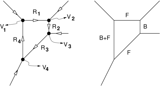
It is easy to check that the resolved web has intersection numbers ±1plus-or-minus1\pm 1 at each vertex and therefore each vertex is an SL(2,𝖹𝖹)𝑆𝐿2𝖹𝖹SL(2,{\sf Z\!\!\!Z}) transform of the basic (1,0)10(1,0), (0,1)01(0,1) and (1,1)11(1,1) vertex. Thus we can decompose any web into pieces which are SL(2,𝖹𝖹)𝑆𝐿2𝖹𝖹SL(2,{\sf Z\!\!\!Z}) transform of the basic three point vertex and the (1,0)10(1,0) 5-brane as shown in Fig. 5 for the case of resolved conifold and local IP2IsuperscriptP2\mbox{I}\!\mbox{P}^{2}.

Refer to caption
Figure 5: a) Resolved conifold, b)local IP2IsuperscriptP2\mbox{I}\!\mbox{P}^{2}. The Riemann surface associated with the web, and the web itself, can be constructed from two basic objects.

In [21] a lattice model interpretation of topological closed string amplitudes was discussed and it was suggested that with a web configuration in which all three point vertices can be converted into four point vertices (in the CY context this corresponds to shrinking IP1IsuperscriptP1\mbox{I}\!\mbox{P}^{1}’s with normal bundle 𝒪(1)𝒪(1)direct-sum𝒪1𝒪1{\cal O}(-1)\oplus{\cal O}(-1)) matrix element R3¯,R4¯|V|R1,R2quantum-operator-product¯subscript𝑅3¯subscript𝑅4𝑉subscript𝑅1subscript𝑅2\langle\bar{R_{3}},\bar{R_{4}}|V|R_{1},R_{2}\rangle should be associated with the four point vertices and propagators elRrsuperscript𝑒subscript𝑙𝑅𝑟e^{-l_{R}r} with the edges. Where |R>ket𝑅|R> are the states of the SU(N)𝑆𝑈𝑁SU(N) WZW theory which are labeled by the highest weight representations R𝑅R at level k+N𝑘𝑁k+N and lRsubscript𝑙𝑅l_{R} is the first Casimir of the representation R𝑅R equal to the number of boxes in the Young-Tableaux of R𝑅R. r𝑟r is the length of the edge and is the Kähler parameter of the associated rational curve in the dual Calabi-Yau. In the case of an external edge we have rmaps-to𝑟r\mapsto\infty and therefore the state associated with the external legs is the vacuum state |0ket0|0\rangle. As discussed in [21] the state |R1,R2ketsubscript𝑅1subscript𝑅2|R_{1},R_{2}\rangle is given by the fusion coefficients,

|R1,R2=RNR1R2R|R,ketsubscript𝑅1subscript𝑅2subscript𝑅subscriptsuperscript𝑁𝑅subscript𝑅1subscript𝑅2ket𝑅\displaystyle|R_{1},R_{2}\rangle=\sum_{R}N^{R}_{R_{1}R_{2}}\,|R\rangle\,, (5)

where the fusion coefficient are given in terms of the modular S𝑆S matrix,

NR1R2R=RSRR1SRR2SRR1S0R.subscriptsuperscript𝑁𝑅subscript𝑅1subscript𝑅2subscriptsuperscript𝑅subscript𝑆superscript𝑅subscript𝑅1subscript𝑆superscript𝑅subscript𝑅2subscriptsuperscript𝑆1superscript𝑅𝑅subscript𝑆0superscript𝑅\displaystyle N^{R}_{R_{1}R_{2}}=\sum_{R^{\prime}}\frac{S_{R^{\prime}R_{1}}S_{R^{\prime}R_{2}}S^{-1}_{R^{\prime}R}}{S_{0R^{\prime}}}\,. (6)

We have seen that three point vertex is more basic than the four point vertex and therefore it is should be possible to associate with it a matrix element R¯3|𝒪|R2,0quantum-operator-productsubscript¯𝑅3𝒪subscript𝑅20\langle\bar{R}_{3}|{\cal O}|R_{2},0\rangle, with 𝒪𝒪{\cal O} being some appropriate operator and |0ket0|0\rangle ,|R2ketsubscript𝑅2|R_{2}\rangle states on the incoming circles and |R3ketsubscript𝑅3|R_{3}\rangle the state on the outgoing circle as shown in Fig. 6. We always consider the vertices in which one of the boundary circles goes of to infinity so that the state on it is the vacuum state.

Refer to caption
Figure 6: a) The vertex, b) the propagator.

We take the amplitude for this vertex to be 111I am grateful to Cumrun Vafa for pointing out a mistake in the definition of the vertex in an earlier version of the preprint.

V(α,β;αβ):=R3¯|S1|R2,0,assign𝑉𝛼𝛽𝛼𝛽quantum-operator-product¯subscript𝑅3superscript𝑆1subscript𝑅20\displaystyle V(\alpha,\beta;\alpha-\beta):=\langle\bar{R_{3}}|S^{-1}|R_{2},0\rangle\,, (7)

where the operator 𝒪=S1𝒪superscript𝑆1{\cal O}=S^{-1} has been chosen such that the corresponding SL(2,𝖹𝖹)𝑆𝐿2𝖹𝖹SL(2,{\sf Z\!\!\!Z}) matrix takes the incoming circle β𝛽\beta into an outgoing circle α𝛼\alpha.222The Riemann surface is embedded in R2×T2superscriptR2superscript𝑇2\mbox{R}^{2}\times T^{2} and α,β𝛼𝛽\alpha,\beta are the basis of H1(T2,𝖹𝖹)subscript𝐻1superscript𝑇2𝖹𝖹H_{1}(T^{2},{\sf Z\!\!\!Z}) such that αβ=1𝛼𝛽1\alpha\cdot\beta=1. The importance of the three point vertex has also been noted in [33] where a vertex with all three circles having non-trivial state has been worked out.

An asymmetrical choice between β𝛽\beta and αβ𝛼𝛽\alpha-\beta was made here. Of the two incoming cycles we choose the one which is followed by the outgoing cycle in the counter clock-wise rotation on the vertex. We will carefully choose our web diagrams from among all SL(2,𝖹𝖹)𝑆𝐿2𝖹𝖹SL(2,{\sf Z\!\!\!Z}) transforms so that the operators at the vertices are of the form TmS1Tksuperscript𝑇𝑚superscript𝑆1superscript𝑇𝑘T^{m}S^{-1}T^{k} for m,k𝖹𝖹𝑚𝑘𝖹𝖹m,k\in{\sf Z\!\!\!Z}. We will see that this is possible for all local del Pezzo surfaces, local Hirzebruch surfaces and their various blowups. This choice is made so that we can use the method given in [21] to calculate the matrix elements R¯|TmS1Tk|Rquantum-operator-product¯𝑅superscript𝑇𝑚superscript𝑆1superscript𝑇𝑘superscript𝑅\langle\bar{R}|T^{m}S^{-1}T^{k}|R^{\prime}\rangle. For the propagator which is cylinder of length r𝑟r with states |R1ketsubscript𝑅1|R_{1}\rangle and |R2ketsubscript𝑅2|R_{2}\rangle at the two boundary circles JR1,JR2H1(T2,𝖹𝖹)subscript𝐽subscript𝑅1subscript𝐽subscript𝑅2subscript𝐻1superscript𝑇2𝖹𝖹J_{R_{1}},J_{R_{2}}\in H_{1}(T^{2},{\sf Z\!\!\!Z}) we choose,

P(JR1,JR2):=elR1rδR1R2.assign𝑃subscript𝐽subscript𝑅1subscript𝐽subscript𝑅2superscript𝑒subscript𝑙subscript𝑅1𝑟subscript𝛿subscript𝑅1subscript𝑅2\displaystyle P(J_{R_{1}},J_{R_{2}}):=e^{-l_{R_{1}}r}\delta_{R_{1}R_{2}}\,. (8)

Although not all web diagrams would allow operators at the vertices of the form TnS1Tmsuperscript𝑇𝑛superscript𝑆1superscript𝑇𝑚T^{n}S^{-1}T^{m} simultaneously we will restrict ourselves to geometries which do allow such vertices so that we can use the results of [21].

The states and the operators we used to define the propagator and the vertices are that of the U(N)𝑈𝑁U(N) WZW theory. It is well known that the primary field of this theory are associated with highest weight representations at level k+N𝑘𝑁k+N [32, 34]. A state |Rket𝑅|R\rangle with weight vector λRsubscript𝜆𝑅\lambda_{R} has conformal dimension

hR=(λR,λR+2ρ)2(k+N)subscript𝑅subscript𝜆𝑅subscript𝜆𝑅2𝜌2𝑘𝑁\displaystyle h_{R}=\frac{(\lambda_{R},\lambda_{R}+2\rho)}{2(k+N)} (9)

where ρ𝜌\rho is one half the sum of positive roots. These states define an orthonormal basis of the Hilbert space of the Chern-Simons theory on a manifold with boundary of genus one, R¯1|R2=δR1,R2inner-productsubscript¯𝑅1subscript𝑅2subscript𝛿subscript𝑅1subscript𝑅2\langle\bar{R}_{1}|R_{2}\rangle=\delta_{R_{1},R_{2}}. As discussed in [32] SL(2,𝖹𝖹)𝑆𝐿2𝖹𝖹SL(2,{\sf Z\!\!\!Z}) action on the boundary T2superscript𝑇2T^{2} is implemented on the Hilbert space using the operators S𝑆S and T𝑇T which form a representation of the SL(2,𝖹𝖹)𝑆𝐿2𝖹𝖹SL(2,{\sf Z\!\!\!Z}),

S2=(ST)3=C,whereCR1,R2=δR1¯,R2.formulae-sequencesuperscript𝑆2superscript𝑆𝑇3𝐶wheresubscript𝐶subscript𝑅1subscript𝑅2subscript𝛿¯subscript𝑅1subscript𝑅2\displaystyle S^{2}=(ST)^{3}=C\,,\,\,\,\mbox{where}\,\,\,\,C_{R_{1},R_{2}}=\delta_{\bar{R_{1}},R_{2}}\,. (10)

In the basis chosen above the T𝑇T operator is diagonal with eigenvalue e2πi(hRc/24)superscript𝑒2𝜋𝑖subscript𝑅𝑐24e^{2\pi i(h_{R}-c/24)} when acting on the state |Rket𝑅|R\rangle. The S𝑆S operator is not diagonal and is given by

SR1,R2:=KwWϵ(w)e2πik+N(w(λR1+ρ),λR2+ρ).assignsubscript𝑆subscript𝑅1subscript𝑅2𝐾subscript𝑤𝑊italic-ϵ𝑤superscript𝑒2𝜋𝑖𝑘𝑁𝑤subscript𝜆subscript𝑅1𝜌subscript𝜆subscript𝑅2𝜌\displaystyle S_{R_{1},R_{2}}:=K\sum_{w\in W}\epsilon(w)e^{-\frac{2\pi i}{k+N}(w(\lambda_{R_{1}+\rho}),\lambda_{R_{2}}+\rho)}\,. (11)

Where K𝐾K only depends on k𝑘k and N𝑁N and W𝑊W is the Weyl group. From the relation between the Hilbert space of the Chern-Simons theory and the space of conformal blocks of the WZW theory [34] it follows that the matrix element WR1,R2:=R¯1|S1|R2assignsubscript𝑊subscript𝑅1subscript𝑅2quantum-operator-productsubscript¯𝑅1superscript𝑆1subscript𝑅2W_{R_{1},R_{2}}:=\langle\bar{R}_{1}|S^{-1}|R_{2}\rangle is the link invariant associated with the Hopf link of linking number +11+1 [21]. This essentially follows from the path integral representation of the matrix element in the Chern-Simons theory. Since the action of T𝑇T is diagonal it follows that [21]

R1¯|TmS1Tn|R2=R1¯|S1|R2(1)mlR1+nlR2q12(mκR2+nκR1),\displaystyle\langle\bar{R_{1}}|T^{m}S^{-1}T^{n}|R_{2}\langle=\langle\bar{R_{1}}|S^{-1}|R_{2}\rangle\,(-1)^{ml_{R_{1}}+nlR_{2}}\,q^{\frac{1}{2}(m\kappa_{R_{2}}+n\kappa_{R_{1}})}\,, (12)

where lRsubscript𝑙𝑅l_{R} as defined before is the number of boxes in the Young-Tableaux of representation R𝑅R and q=e2πik+N𝑞superscript𝑒2𝜋𝑖𝑘𝑁q=e^{\frac{2\pi i}{k+N}}. The integers κRsubscript𝜅𝑅\kappa_{R} are defined in terms of the number of rows d(μR)𝑑superscript𝜇𝑅d(\mu^{R}) in the Young Tableaux μRsuperscript𝜇𝑅\mu^{R} and number of boxes in a a given row μiRsubscriptsuperscript𝜇𝑅𝑖\mu^{R}_{i} as

κR=lR+i=1d(μR)μiR(μiR2i).subscript𝜅𝑅subscript𝑙𝑅superscriptsubscript𝑖1𝑑superscript𝜇𝑅subscriptsuperscript𝜇𝑅𝑖subscriptsuperscript𝜇𝑅𝑖2𝑖\displaystyle\kappa_{R}=l_{R}+\sum_{i=1}^{d(\mu^{R})}\mu^{R}_{i}(\mu^{R}_{i}-2i). (13)

Thus we only need to calculate the matrix elements of S1superscript𝑆1S^{-1} which can be done easily using the results of [35, 36, 21] as we will explain now.

WR1,R2subscript𝑊subscript𝑅1subscript𝑅2W_{R_{1},R_{2}}: The matrix element is a function of q𝑞q and λ:=qNassign𝜆superscript𝑞𝑁\lambda:=q^{N}. It is defined using the following q-numbers,

[x]:=qx2qx2,[x]λ=λ12qx2λ12qx2,formulae-sequenceassigndelimited-[]𝑥superscript𝑞𝑥2superscript𝑞𝑥2subscriptdelimited-[]𝑥𝜆superscript𝜆12superscript𝑞𝑥2superscript𝜆12superscript𝑞𝑥2\displaystyle[x]:=q^{\frac{x}{2}}-q^{-\frac{x}{2}}\,,\,\,[x]_{\lambda}=\lambda^{\frac{1}{2}}q^{\frac{x}{2}}-\lambda^{-\frac{1}{2}}q^{\frac{x}{2}}\,, (14)

and a polynomial associated with each Young-Tableaux μRsuperscript𝜇𝑅\mu^{R} given by

sμR(P(t))=deti,jeμ^iR+ji,e0=1,ek<0=0.formulae-sequencesubscript𝑠superscript𝜇𝑅𝑃𝑡subscriptdet𝑖𝑗subscript𝑒subscriptsuperscript^𝜇𝑅𝑖𝑗𝑖formulae-sequencesubscript𝑒01subscript𝑒𝑘00\displaystyle s_{\mu^{R}}(P(t))=\mbox{det}_{i,j}e_{\widehat{\mu}^{R}_{i}+j-i}\,,\,\,\,e_{0}=1,\,\,e_{k<0}=0\,. (15)

Where μ^Rsuperscript^𝜇𝑅\widehat{\mu}^{R} is the Young-Tableaux obtained by interchanging the rows and the columns and eisubscript𝑒𝑖e_{i} are such that P(t)=1+n=1entn𝑃𝑡1superscriptsubscript𝑛1subscript𝑒𝑛superscript𝑡𝑛P(t)=1+\sum_{n=1}^{\infty}e_{n}t^{n}. For example,

s subscript𝑠 \displaystyle s_{\vbox{\offinterlineskip\kern 1.0pt\hbox{\kern 1.0pt\vbox{\hbox{\noindent\vbox{\hbox{\vbox to0.0pt{\hrule height=0.4pt,width=3.90555pt\vss}}\hbox{\vbox{\hbox to0.0pt{\vrule width=0.4pt,height=3.90555pt\hss}}\kern 3.90555pt\vbox{\hbox to0.0pt{\vrule width=0.4pt,height=3.90555pt\hss}}}\hbox{\vbox{\hbox{\vbox to0.0pt{\hrule height=0.4pt,width=4.30554pt\vss}}}\kern-0.4pt}}}\hbox{}}\kern 1.0pt\kern 0.4pt}\kern 1.0pt\kern 0.4pt}} =\displaystyle= e1,s =e12e2,s =e2,formulae-sequencesubscript𝑒1subscript𝑠 superscriptsubscript𝑒12subscript𝑒2subscript𝑠 subscript𝑒2\displaystyle e_{1}\,,\,s_{\vbox{\offinterlineskip\kern 1.0pt\hbox{\kern 1.0pt\vbox{\hbox{\noindent\vbox{\hbox{\vbox to0.0pt{\hrule height=0.4pt,width=3.90555pt\vss}}\hbox{\vbox{\hbox to0.0pt{\vrule width=0.4pt,height=3.90555pt\hss}}\kern 3.90555pt\vbox{\hbox to0.0pt{\vrule width=0.4pt,height=3.90555pt\hss}}}\hbox{\vbox{\hbox{\vbox to0.0pt{\hrule height=0.4pt,width=4.30554pt\vss}}}\kern-0.4pt}}\vbox{\hbox{\vbox to0.0pt{\hrule height=0.4pt,width=3.90555pt\vss}}\hbox{\vbox{\hbox to0.0pt{\vrule width=0.4pt,height=3.90555pt\hss}}\kern 3.90555pt\vbox{\hbox to0.0pt{\vrule width=0.4pt,height=3.90555pt\hss}}}\hbox{\vbox{\hbox{\vbox to0.0pt{\hrule height=0.4pt,width=4.30554pt\vss}}}\kern-0.4pt}}}\hbox{}}\kern 1.0pt\kern 0.4pt}\kern 1.0pt\kern 0.4pt}}=e_{1}^{2}-e_{2}\,,\,\,s_{\vbox{\offinterlineskip\kern 1.0pt\hbox{\kern 1.0pt\vbox{\hbox{\noindent\vbox{\hbox{\vbox to0.0pt{\hrule height=0.4pt,width=3.90555pt\vss}}\hbox{\vbox{\hbox to0.0pt{\vrule width=0.4pt,height=3.90555pt\hss}}\kern 3.90555pt\vbox{\hbox to0.0pt{\vrule width=0.4pt,height=3.90555pt\hss}}}\hbox{\vbox{\hbox{\vbox to0.0pt{\hrule height=0.4pt,width=4.30554pt\vss}}}\kern-0.4pt}}}\hbox{\noindent\vbox{\hbox{\vbox to0.0pt{\hrule height=0.4pt,width=3.90555pt\vss}}\hbox{\vbox{\hbox to0.0pt{\vrule width=0.4pt,height=3.90555pt\hss}}\kern 3.90555pt\vbox{\hbox to0.0pt{\vrule width=0.4pt,height=3.90555pt\hss}}}\hbox{\vbox{\hbox{\vbox to0.0pt{\hrule height=0.4pt,width=4.30554pt\vss}}}\kern-0.4pt}}}\hbox{}}\kern 1.0pt\kern 0.4pt}\kern 1.0pt\kern 0.4pt}}=e_{2}\,,\,\, (16)
s subscript𝑠 \displaystyle s_{\vbox{\offinterlineskip\kern 1.0pt\hbox{\kern 1.0pt\vbox{\hbox{\noindent\vbox{\hbox{\vbox to0.0pt{\hrule height=0.4pt,width=3.90555pt\vss}}\hbox{\vbox{\hbox to0.0pt{\vrule width=0.4pt,height=3.90555pt\hss}}\kern 3.90555pt\vbox{\hbox to0.0pt{\vrule width=0.4pt,height=3.90555pt\hss}}}\hbox{\vbox{\hbox{\vbox to0.0pt{\hrule height=0.4pt,width=4.30554pt\vss}}}\kern-0.4pt}}\vbox{\hbox{\vbox to0.0pt{\hrule height=0.4pt,width=3.90555pt\vss}}\hbox{\vbox{\hbox to0.0pt{\vrule width=0.4pt,height=3.90555pt\hss}}\kern 3.90555pt\vbox{\hbox to0.0pt{\vrule width=0.4pt,height=3.90555pt\hss}}}\hbox{\vbox{\hbox{\vbox to0.0pt{\hrule height=0.4pt,width=4.30554pt\vss}}}\kern-0.4pt}}\vbox{\hbox{\vbox to0.0pt{\hrule height=0.4pt,width=3.90555pt\vss}}\hbox{\vbox{\hbox to0.0pt{\vrule width=0.4pt,height=3.90555pt\hss}}\kern 3.90555pt\vbox{\hbox to0.0pt{\vrule width=0.4pt,height=3.90555pt\hss}}}\hbox{\vbox{\hbox{\vbox to0.0pt{\hrule height=0.4pt,width=4.30554pt\vss}}}\kern-0.4pt}}}\hbox{}}\kern 1.0pt\kern 0.4pt}\kern 1.0pt\kern 0.4pt}} =\displaystyle= e32e1e2+e13,s =e3,s =e3e1e2.formulae-sequencesubscript𝑒32subscript𝑒1subscript𝑒2superscriptsubscript𝑒13subscript𝑠 subscript𝑒3subscript𝑠 subscript𝑒3subscript𝑒1subscript𝑒2\displaystyle e_{3}-2e_{1}e_{2}+e_{1}^{3}\,,\,\,s_{\vbox{\offinterlineskip\kern 1.0pt\hbox{\kern 1.0pt\vbox{\hbox{\noindent\vbox{\hbox{\vbox to0.0pt{\hrule height=0.4pt,width=3.90555pt\vss}}\hbox{\vbox{\hbox to0.0pt{\vrule width=0.4pt,height=3.90555pt\hss}}\kern 3.90555pt\vbox{\hbox to0.0pt{\vrule width=0.4pt,height=3.90555pt\hss}}}\hbox{\vbox{\hbox{\vbox to0.0pt{\hrule height=0.4pt,width=4.30554pt\vss}}}\kern-0.4pt}}}\hbox{\noindent\vbox{\hbox{\vbox to0.0pt{\hrule height=0.4pt,width=3.90555pt\vss}}\hbox{\vbox{\hbox to0.0pt{\vrule width=0.4pt,height=3.90555pt\hss}}\kern 3.90555pt\vbox{\hbox to0.0pt{\vrule width=0.4pt,height=3.90555pt\hss}}}\hbox{\vbox{\hbox{\vbox to0.0pt{\hrule height=0.4pt,width=4.30554pt\vss}}}\kern-0.4pt}}}\hbox{\noindent\vbox{\hbox{\vbox to0.0pt{\hrule height=0.4pt,width=3.90555pt\vss}}\hbox{\vbox{\hbox to0.0pt{\vrule width=0.4pt,height=3.90555pt\hss}}\kern 3.90555pt\vbox{\hbox to0.0pt{\vrule width=0.4pt,height=3.90555pt\hss}}}\hbox{\vbox{\hbox{\vbox to0.0pt{\hrule height=0.4pt,width=4.30554pt\vss}}}\kern-0.4pt}}}\hbox{}}\kern 1.0pt\kern 0.4pt}\kern 1.0pt\kern 0.4pt}}=e_{3}\,,\,\,s_{\vbox{\offinterlineskip\kern 1.0pt\hbox{\kern 1.0pt\vbox{\hbox{\noindent\vbox{\hbox{\vbox to0.0pt{\hrule height=0.4pt,width=3.90555pt\vss}}\hbox{\vbox{\hbox to0.0pt{\vrule width=0.4pt,height=3.90555pt\hss}}\kern 3.90555pt\vbox{\hbox to0.0pt{\vrule width=0.4pt,height=3.90555pt\hss}}}\hbox{\vbox{\hbox{\vbox to0.0pt{\hrule height=0.4pt,width=4.30554pt\vss}}}\kern-0.4pt}}\vbox{\hbox{\vbox to0.0pt{\hrule height=0.4pt,width=3.90555pt\vss}}\hbox{\vbox{\hbox to0.0pt{\vrule width=0.4pt,height=3.90555pt\hss}}\kern 3.90555pt\vbox{\hbox to0.0pt{\vrule width=0.4pt,height=3.90555pt\hss}}}\hbox{\vbox{\hbox{\vbox to0.0pt{\hrule height=0.4pt,width=4.30554pt\vss}}}\kern-0.4pt}}}\hbox{\noindent\vbox{\hbox{\vbox to0.0pt{\hrule height=0.4pt,width=3.90555pt\vss}}\hbox{\vbox{\hbox to0.0pt{\vrule width=0.4pt,height=3.90555pt\hss}}\kern 3.90555pt\vbox{\hbox to0.0pt{\vrule width=0.4pt,height=3.90555pt\hss}}}\hbox{\vbox{\hbox{\vbox to0.0pt{\hrule height=0.4pt,width=4.30554pt\vss}}}\kern-0.4pt}}}\hbox{}}\kern 1.0pt\kern 0.4pt}\kern 1.0pt\kern 0.4pt}}=e_{3}-e_{1}e_{2}\,.

The matrix element WR1,R2subscript𝑊subscript𝑅1subscript𝑅2W_{R_{1},R_{2}} is given by [35, 36, 21]

WR1,R2:=dimqR1(λq)lR22sμR2(EμR1(t)).assignsubscript𝑊subscript𝑅1subscript𝑅2subscriptdim𝑞subscript𝑅1superscript𝜆𝑞subscript𝑙subscript𝑅22subscript𝑠superscript𝜇subscript𝑅2subscript𝐸superscript𝜇subscript𝑅1𝑡\displaystyle W_{R_{1},R_{2}}:=\mbox{dim}_{q}R_{1}\,(\lambda\,q)^{\frac{l_{R_{2}}}{2}}\,s_{\mu^{R_{2}}}(E_{\mu^{R_{1}}}(t))\,. (17)

Where

dimqR:=1i<jd(μR)[μiμj+ji][ji]i=1d(μR)v=i+1μii[v]λv=1μi[vi+d(μR)].assignsubscriptdim𝑞𝑅subscriptproduct1𝑖𝑗𝑑superscript𝜇𝑅delimited-[]subscript𝜇𝑖subscript𝜇𝑗𝑗𝑖delimited-[]𝑗𝑖superscriptsubscriptproduct𝑖1𝑑superscript𝜇𝑅superscriptsubscriptproduct𝑣𝑖1subscript𝜇𝑖𝑖subscriptdelimited-[]𝑣𝜆superscriptsubscriptproduct𝑣1subscript𝜇𝑖delimited-[]𝑣𝑖𝑑superscript𝜇𝑅\displaystyle\mbox{dim}_{q}R:=\prod_{1\leq i<j\leq d(\mu^{R})}\frac{[\mu_{i}-\mu_{j}+j-i]}{[j-i]}\prod_{i=1}^{d(\mu^{R})}\frac{\prod_{v=-i+1}^{\mu_{i}-i}[v]_{\lambda}}{\prod_{v=1}^{\mu_{i}}[v-i+d(\mu^{R})]}\,. (18)

and

EμR(t)=(j=1d(μR)1+qμjjt1+qjt)(1+n=1(i=1n1λ1qi1qi1)tn).subscript𝐸superscript𝜇𝑅𝑡superscriptsubscriptproduct𝑗1𝑑superscript𝜇𝑅1superscript𝑞subscript𝜇𝑗𝑗𝑡1superscript𝑞𝑗𝑡1superscriptsubscript𝑛1superscriptsubscriptproduct𝑖1𝑛1superscript𝜆1superscript𝑞𝑖1superscript𝑞𝑖1superscript𝑡𝑛\displaystyle E_{\mu^{R}}(t)=(\prod_{j=1}^{d(\mu^{R})}\frac{1+q^{\mu_{j}-j}t}{1+q^{-j}t})\,(1+\sum_{n=1}^{\infty}(\prod_{i=1}^{n}\frac{1-\lambda^{-1}q^{i-1}}{q^{i}-1})t^{n})\,. (19)

We will see later that in the large N𝑁N limit keeping q𝑞q fixed we will only need the leading order term, coefficient of λlR1+lR22superscript𝜆subscript𝑙subscript𝑅1subscript𝑙subscript𝑅22\lambda^{\frac{l_{R_{1}}+l_{R_{2}}}{2}}, in WR1,R2subscript𝑊subscript𝑅1subscript𝑅2W_{R_{1},R_{2}} which we denote by 𝒲R1,R2subscript𝒲subscript𝑅1subscript𝑅2{\cal W}_{R_{1},R_{2}}. It is easy to calculate the leading order term since the expression for E0(t)subscript𝐸0𝑡E_{0}(t) simplifies in this limit and because the leading order term in dimqRsubscriptdim𝑞𝑅\mbox{dim}_{q}R can be explicitly calculated and is given by [21]

qκR/41i<jd(μR)[μiμj+ji][ji]i=1d(R)v=1μi1[vi+d(μR)].superscript𝑞subscript𝜅𝑅4subscriptproduct1𝑖𝑗𝑑superscript𝜇𝑅delimited-[]subscript𝜇𝑖subscript𝜇𝑗𝑗𝑖delimited-[]𝑗𝑖superscriptsubscriptproduct𝑖1𝑑𝑅superscriptsubscriptproduct𝑣1subscript𝜇𝑖1delimited-[]𝑣𝑖𝑑superscript𝜇𝑅\displaystyle q^{\kappa_{R}/4}\,\prod_{1\leq i<j\leq d(\mu^{R})}\frac{[\mu_{i}-\mu_{j}+j-i]}{[j-i]}\prod_{i=1}^{d(R)}\prod_{v=1}^{\mu_{i}}\frac{1}{[v-i+d(\mu^{R})]}\,. (20)

We list here 𝒲R1,R2subscript𝒲subscript𝑅1subscript𝑅2{\cal W}_{R_{1},R_{2}} for a few representations which we will need later for computing integer invariants.

𝒲 nsubscript𝒲subscript 𝑛\displaystyle{\cal W}_{\underbrace{\vbox{\offinterlineskip\kern 1.0pt\hbox{\kern 1.0pt\vbox{\hbox{\noindent\vbox{\hbox{\vbox to0.0pt{\hrule height=0.4pt,width=3.90555pt\vss}}\hbox{\vbox{\hbox to0.0pt{\vrule width=0.4pt,height=3.90555pt\hss}}\kern 3.90555pt\vbox{\hbox to0.0pt{\vrule width=0.4pt,height=3.90555pt\hss}}}\hbox{\vbox{\hbox{\vbox to0.0pt{\hrule height=0.4pt,width=4.30554pt\vss}}}\kern-0.4pt}}\vbox{\hbox{\vbox to0.0pt{\hrule height=0.4pt,width=3.90555pt\vss}}\hbox{\vbox{\hbox to0.0pt{\vrule width=0.4pt,height=3.90555pt\hss}}\kern 3.90555pt\vbox{\hbox to0.0pt{\vrule width=0.4pt,height=3.90555pt\hss}}}\hbox{\vbox{\hbox{\vbox to0.0pt{\hrule height=0.4pt,width=4.30554pt\vss}}}\kern-0.4pt}}\vbox{\hbox{\vbox to0.0pt{\hrule height=0.4pt,width=3.90555pt\vss}}\hbox{\vbox{\hbox to0.0pt{\vrule width=0.4pt,height=3.90555pt\hss}}\kern 3.90555pt\vbox{\hbox to0.0pt{\vrule width=0.4pt,height=3.90555pt\hss}}}\hbox{\vbox{\hbox{\vbox to0.0pt{\hrule height=0.4pt,width=4.30554pt\vss}}}\kern-0.4pt}}}\hbox{}}\kern 1.0pt\kern 0.4pt}\kern 1.0pt\kern 0.4pt}\cdots\vbox{\offinterlineskip\kern 1.0pt\hbox{\kern 1.0pt\vbox{\hbox{\noindent\vbox{\hbox{\vbox to0.0pt{\hrule height=0.4pt,width=3.90555pt\vss}}\hbox{\vbox{\hbox to0.0pt{\vrule width=0.4pt,height=3.90555pt\hss}}\kern 3.90555pt\vbox{\hbox to0.0pt{\vrule width=0.4pt,height=3.90555pt\hss}}}\hbox{\vbox{\hbox{\vbox to0.0pt{\hrule height=0.4pt,width=4.30554pt\vss}}}\kern-0.4pt}}}\hbox{}}\kern 1.0pt\kern 0.4pt}\kern 1.0pt\kern 0.4pt}}_{n}} =\displaystyle= qn(n1)/4k=1n(qk/2qk/2),superscript𝑞𝑛𝑛14superscriptsubscriptproduct𝑘1𝑛superscript𝑞𝑘2superscript𝑞𝑘2\displaystyle\frac{q^{n(n-1)/4}}{\prod_{k=1}^{n}(q^{k/2}-q^{-k/2})}\,, (21)
𝒲Ansubscript𝒲subscript𝐴𝑛\displaystyle{\cal W}_{A_{n}} =\displaystyle= qn(n1)/4k=1n(qk/2qk/2),superscript𝑞𝑛𝑛14superscriptsubscriptproduct𝑘1𝑛superscript𝑞𝑘2superscript𝑞𝑘2\displaystyle\frac{q^{-n(n-1)/4}}{\prod_{k=1}^{n}(q^{k/2}-q^{-k/2})}\,,
𝒲 , subscript𝒲 \displaystyle{\cal W}_{\vbox{\offinterlineskip\kern 1.0pt\hbox{\kern 1.0pt\vbox{\hbox{\noindent\vbox{\hbox{\vbox to0.0pt{\hrule height=0.4pt,width=3.90555pt\vss}}\hbox{\vbox{\hbox to0.0pt{\vrule width=0.4pt,height=3.90555pt\hss}}\kern 3.90555pt\vbox{\hbox to0.0pt{\vrule width=0.4pt,height=3.90555pt\hss}}}\hbox{\vbox{\hbox{\vbox to0.0pt{\hrule height=0.4pt,width=4.30554pt\vss}}}\kern-0.4pt}}}\hbox{}}\kern 1.0pt\kern 0.4pt}\kern 1.0pt\kern 0.4pt},\vbox{\offinterlineskip\kern 1.0pt\hbox{\kern 1.0pt\vbox{\hbox{\noindent\vbox{\hbox{\vbox to0.0pt{\hrule height=0.4pt,width=3.90555pt\vss}}\hbox{\vbox{\hbox to0.0pt{\vrule width=0.4pt,height=3.90555pt\hss}}\kern 3.90555pt\vbox{\hbox to0.0pt{\vrule width=0.4pt,height=3.90555pt\hss}}}\hbox{\vbox{\hbox{\vbox to0.0pt{\hrule height=0.4pt,width=4.30554pt\vss}}}\kern-0.4pt}}}\hbox{}}\kern 1.0pt\kern 0.4pt}\kern 1.0pt\kern 0.4pt}} =\displaystyle= ((q+q11)(q1/2q1/2)2)\displaystyle\frac{((q+q^{-1}-1)}{(q^{1/2}-q^{-1/2})^{2}})\,
𝒲 , subscript𝒲 \displaystyle{\cal W}_{\vbox{\offinterlineskip\kern 1.0pt\hbox{\kern 1.0pt\vbox{\hbox{\noindent\vbox{\hbox{\vbox to0.0pt{\hrule height=0.4pt,width=3.90555pt\vss}}\hbox{\vbox{\hbox to0.0pt{\vrule width=0.4pt,height=3.90555pt\hss}}\kern 3.90555pt\vbox{\hbox to0.0pt{\vrule width=0.4pt,height=3.90555pt\hss}}}\hbox{\vbox{\hbox{\vbox to0.0pt{\hrule height=0.4pt,width=4.30554pt\vss}}}\kern-0.4pt}}\vbox{\hbox{\vbox to0.0pt{\hrule height=0.4pt,width=3.90555pt\vss}}\hbox{\vbox{\hbox to0.0pt{\vrule width=0.4pt,height=3.90555pt\hss}}\kern 3.90555pt\vbox{\hbox to0.0pt{\vrule width=0.4pt,height=3.90555pt\hss}}}\hbox{\vbox{\hbox{\vbox to0.0pt{\hrule height=0.4pt,width=4.30554pt\vss}}}\kern-0.4pt}}}\hbox{}}\kern 1.0pt\kern 0.4pt}\kern 1.0pt\kern 0.4pt},\vbox{\offinterlineskip\kern 1.0pt\hbox{\kern 1.0pt\vbox{\hbox{\noindent\vbox{\hbox{\vbox to0.0pt{\hrule height=0.4pt,width=3.90555pt\vss}}\hbox{\vbox{\hbox to0.0pt{\vrule width=0.4pt,height=3.90555pt\hss}}\kern 3.90555pt\vbox{\hbox to0.0pt{\vrule width=0.4pt,height=3.90555pt\hss}}}\hbox{\vbox{\hbox{\vbox to0.0pt{\hrule height=0.4pt,width=4.30554pt\vss}}}\kern-0.4pt}}}\hbox{}}\kern 1.0pt\kern 0.4pt}\kern 1.0pt\kern 0.4pt}} =\displaystyle= 1(q1/2q1/2)3(1q2+q3)1+q1superscriptsuperscript𝑞12superscript𝑞1231superscript𝑞2superscript𝑞31𝑞\displaystyle\frac{1}{(q^{1/2}-q^{-1/2})^{3}}\,\frac{(1-q^{2}+q^{3})}{1+q}
𝒲 , subscript𝒲 \displaystyle{\cal W}_{\vbox{\offinterlineskip\kern 1.0pt\hbox{\kern 1.0pt\vbox{\hbox{\noindent\vbox{\hbox{\vbox to0.0pt{\hrule height=0.4pt,width=3.90555pt\vss}}\hbox{\vbox{\hbox to0.0pt{\vrule width=0.4pt,height=3.90555pt\hss}}\kern 3.90555pt\vbox{\hbox to0.0pt{\vrule width=0.4pt,height=3.90555pt\hss}}}\hbox{\vbox{\hbox{\vbox to0.0pt{\hrule height=0.4pt,width=4.30554pt\vss}}}\kern-0.4pt}}}\hbox{\noindent\vbox{\hbox{\vbox to0.0pt{\hrule height=0.4pt,width=3.90555pt\vss}}\hbox{\vbox{\hbox to0.0pt{\vrule width=0.4pt,height=3.90555pt\hss}}\kern 3.90555pt\vbox{\hbox to0.0pt{\vrule width=0.4pt,height=3.90555pt\hss}}}\hbox{\vbox{\hbox{\vbox to0.0pt{\hrule height=0.4pt,width=4.30554pt\vss}}}\kern-0.4pt}}}\hbox{}}\kern 1.0pt\kern 0.4pt}\kern 1.0pt\kern 0.4pt},\vbox{\offinterlineskip\kern 1.0pt\hbox{\kern 1.0pt\vbox{\hbox{\noindent\vbox{\hbox{\vbox to0.0pt{\hrule height=0.4pt,width=3.90555pt\vss}}\hbox{\vbox{\hbox to0.0pt{\vrule width=0.4pt,height=3.90555pt\hss}}\kern 3.90555pt\vbox{\hbox to0.0pt{\vrule width=0.4pt,height=3.90555pt\hss}}}\hbox{\vbox{\hbox{\vbox to0.0pt{\hrule height=0.4pt,width=4.30554pt\vss}}}\kern-0.4pt}}}\hbox{}}\kern 1.0pt\kern 0.4pt}\kern 1.0pt\kern 0.4pt}} =\displaystyle= 1(q1/2q1/2)3q2(1q+q3)1+q1superscriptsuperscript𝑞12superscript𝑞123superscript𝑞21𝑞superscript𝑞31𝑞\displaystyle\frac{1}{(q^{1/2}-q^{-1/2})^{3}}\,\frac{q^{-2}(1-q+q^{3})}{1+q}
𝒲 , subscript𝒲 \displaystyle{\cal W}_{\vbox{\offinterlineskip\kern 1.0pt\hbox{\kern 1.0pt\vbox{\hbox{\noindent\vbox{\hbox{\vbox to0.0pt{\hrule height=0.4pt,width=3.90555pt\vss}}\hbox{\vbox{\hbox to0.0pt{\vrule width=0.4pt,height=3.90555pt\hss}}\kern 3.90555pt\vbox{\hbox to0.0pt{\vrule width=0.4pt,height=3.90555pt\hss}}}\hbox{\vbox{\hbox{\vbox to0.0pt{\hrule height=0.4pt,width=4.30554pt\vss}}}\kern-0.4pt}}\vbox{\hbox{\vbox to0.0pt{\hrule height=0.4pt,width=3.90555pt\vss}}\hbox{\vbox{\hbox to0.0pt{\vrule width=0.4pt,height=3.90555pt\hss}}\kern 3.90555pt\vbox{\hbox to0.0pt{\vrule width=0.4pt,height=3.90555pt\hss}}}\hbox{\vbox{\hbox{\vbox to0.0pt{\hrule height=0.4pt,width=4.30554pt\vss}}}\kern-0.4pt}}\vbox{\hbox{\vbox to0.0pt{\hrule height=0.4pt,width=3.90555pt\vss}}\hbox{\vbox{\hbox to0.0pt{\vrule width=0.4pt,height=3.90555pt\hss}}\kern 3.90555pt\vbox{\hbox to0.0pt{\vrule width=0.4pt,height=3.90555pt\hss}}}\hbox{\vbox{\hbox{\vbox to0.0pt{\hrule height=0.4pt,width=4.30554pt\vss}}}\kern-0.4pt}}}\hbox{}}\kern 1.0pt\kern 0.4pt}\kern 1.0pt\kern 0.4pt},\vbox{\offinterlineskip\kern 1.0pt\hbox{\kern 1.0pt\vbox{\hbox{\noindent\vbox{\hbox{\vbox to0.0pt{\hrule height=0.4pt,width=3.90555pt\vss}}\hbox{\vbox{\hbox to0.0pt{\vrule width=0.4pt,height=3.90555pt\hss}}\kern 3.90555pt\vbox{\hbox to0.0pt{\vrule width=0.4pt,height=3.90555pt\hss}}}\hbox{\vbox{\hbox{\vbox to0.0pt{\hrule height=0.4pt,width=4.30554pt\vss}}}\kern-0.4pt}}}\hbox{}}\kern 1.0pt\kern 0.4pt}\kern 1.0pt\kern 0.4pt}} =\displaystyle= 1(q1/2q1/2)4q2(1q3+q4)(1+q)(1+q+q2)1superscriptsuperscript𝑞12superscript𝑞124superscript𝑞21superscript𝑞3superscript𝑞41𝑞1𝑞superscript𝑞2\displaystyle\frac{1}{(q^{1/2}-q^{-1/2})^{4}}\,\frac{q^{2}(1-q^{3}+q^{4})}{(1+q)(1+q+q^{2})}
𝒲 , subscript𝒲 \displaystyle{\cal W}_{\vbox{\offinterlineskip\kern 1.0pt\hbox{\kern 1.0pt\vbox{\hbox{\noindent\vbox{\hbox{\vbox to0.0pt{\hrule height=0.4pt,width=3.90555pt\vss}}\hbox{\vbox{\hbox to0.0pt{\vrule width=0.4pt,height=3.90555pt\hss}}\kern 3.90555pt\vbox{\hbox to0.0pt{\vrule width=0.4pt,height=3.90555pt\hss}}}\hbox{\vbox{\hbox{\vbox to0.0pt{\hrule height=0.4pt,width=4.30554pt\vss}}}\kern-0.4pt}}\vbox{\hbox{\vbox to0.0pt{\hrule height=0.4pt,width=3.90555pt\vss}}\hbox{\vbox{\hbox to0.0pt{\vrule width=0.4pt,height=3.90555pt\hss}}\kern 3.90555pt\vbox{\hbox to0.0pt{\vrule width=0.4pt,height=3.90555pt\hss}}}\hbox{\vbox{\hbox{\vbox to0.0pt{\hrule height=0.4pt,width=4.30554pt\vss}}}\kern-0.4pt}}}\hbox{\noindent\vbox{\hbox{\vbox to0.0pt{\hrule height=0.4pt,width=3.90555pt\vss}}\hbox{\vbox{\hbox to0.0pt{\vrule width=0.4pt,height=3.90555pt\hss}}\kern 3.90555pt\vbox{\hbox to0.0pt{\vrule width=0.4pt,height=3.90555pt\hss}}}\hbox{\vbox{\hbox{\vbox to0.0pt{\hrule height=0.4pt,width=4.30554pt\vss}}}\kern-0.4pt}}}\hbox{}}\kern 1.0pt\kern 0.4pt}\kern 1.0pt\kern 0.4pt},\vbox{\offinterlineskip\kern 1.0pt\hbox{\kern 1.0pt\vbox{\hbox{\noindent\vbox{\hbox{\vbox to0.0pt{\hrule height=0.4pt,width=3.90555pt\vss}}\hbox{\vbox{\hbox to0.0pt{\vrule width=0.4pt,height=3.90555pt\hss}}\kern 3.90555pt\vbox{\hbox to0.0pt{\vrule width=0.4pt,height=3.90555pt\hss}}}\hbox{\vbox{\hbox{\vbox to0.0pt{\hrule height=0.4pt,width=4.30554pt\vss}}}\kern-0.4pt}}}\hbox{}}\kern 1.0pt\kern 0.4pt}\kern 1.0pt\kern 0.4pt}} =\displaystyle= 1(q1/2q1/2)41q+q2q3+q41+q+q2,1superscriptsuperscript𝑞12superscript𝑞1241𝑞superscript𝑞2superscript𝑞3superscript𝑞41𝑞superscript𝑞2\displaystyle\frac{1}{(q^{1/2}-q^{-1/2})^{4}}\,\frac{1-q+q^{2}-q^{3}+q^{4}}{1+q+q^{2}}\,,
𝒲 , subscript𝒲 \displaystyle{\cal W}_{\vbox{\offinterlineskip\kern 1.0pt\hbox{\kern 1.0pt\vbox{\hbox{\noindent\vbox{\hbox{\vbox to0.0pt{\hrule height=0.4pt,width=3.90555pt\vss}}\hbox{\vbox{\hbox to0.0pt{\vrule width=0.4pt,height=3.90555pt\hss}}\kern 3.90555pt\vbox{\hbox to0.0pt{\vrule width=0.4pt,height=3.90555pt\hss}}}\hbox{\vbox{\hbox{\vbox to0.0pt{\hrule height=0.4pt,width=4.30554pt\vss}}}\kern-0.4pt}}}\hbox{\noindent\vbox{\hbox{\vbox to0.0pt{\hrule height=0.4pt,width=3.90555pt\vss}}\hbox{\vbox{\hbox to0.0pt{\vrule width=0.4pt,height=3.90555pt\hss}}\kern 3.90555pt\vbox{\hbox to0.0pt{\vrule width=0.4pt,height=3.90555pt\hss}}}\hbox{\vbox{\hbox{\vbox to0.0pt{\hrule height=0.4pt,width=4.30554pt\vss}}}\kern-0.4pt}}}\hbox{\noindent\vbox{\hbox{\vbox to0.0pt{\hrule height=0.4pt,width=3.90555pt\vss}}\hbox{\vbox{\hbox to0.0pt{\vrule width=0.4pt,height=3.90555pt\hss}}\kern 3.90555pt\vbox{\hbox to0.0pt{\vrule width=0.4pt,height=3.90555pt\hss}}}\hbox{\vbox{\hbox{\vbox to0.0pt{\hrule height=0.4pt,width=4.30554pt\vss}}}\kern-0.4pt}}}\hbox{}}\kern 1.0pt\kern 0.4pt}\kern 1.0pt\kern 0.4pt},\vbox{\offinterlineskip\kern 1.0pt\hbox{\kern 1.0pt\vbox{\hbox{\noindent\vbox{\hbox{\vbox to0.0pt{\hrule height=0.4pt,width=3.90555pt\vss}}\hbox{\vbox{\hbox to0.0pt{\vrule width=0.4pt,height=3.90555pt\hss}}\kern 3.90555pt\vbox{\hbox to0.0pt{\vrule width=0.4pt,height=3.90555pt\hss}}}\hbox{\vbox{\hbox{\vbox to0.0pt{\hrule height=0.4pt,width=4.30554pt\vss}}}\kern-0.4pt}}}\hbox{}}\kern 1.0pt\kern 0.4pt}\kern 1.0pt\kern 0.4pt}} =\displaystyle= 1(q1/2q1/2)4q1/2(1q+q4)(1+q)(1+q+q2)1superscriptsuperscript𝑞12superscript𝑞124superscript𝑞121𝑞superscript𝑞41𝑞1𝑞superscript𝑞2\displaystyle\frac{1}{(q^{1/2}-q^{-1/2})^{4}}\,\frac{q^{1/2}(1-q+q^{4})}{(1+q)(1+q+q^{2})}\,
𝒲 , subscript𝒲 \displaystyle{\cal W}_{\vbox{\offinterlineskip\kern 1.0pt\hbox{\kern 1.0pt\vbox{\hbox{\noindent\vbox{\hbox{\vbox to0.0pt{\hrule height=0.4pt,width=3.90555pt\vss}}\hbox{\vbox{\hbox to0.0pt{\vrule width=0.4pt,height=3.90555pt\hss}}\kern 3.90555pt\vbox{\hbox to0.0pt{\vrule width=0.4pt,height=3.90555pt\hss}}}\hbox{\vbox{\hbox{\vbox to0.0pt{\hrule height=0.4pt,width=4.30554pt\vss}}}\kern-0.4pt}}\vbox{\hbox{\vbox to0.0pt{\hrule height=0.4pt,width=3.90555pt\vss}}\hbox{\vbox{\hbox to0.0pt{\vrule width=0.4pt,height=3.90555pt\hss}}\kern 3.90555pt\vbox{\hbox to0.0pt{\vrule width=0.4pt,height=3.90555pt\hss}}}\hbox{\vbox{\hbox{\vbox to0.0pt{\hrule height=0.4pt,width=4.30554pt\vss}}}\kern-0.4pt}}}\hbox{}}\kern 1.0pt\kern 0.4pt}\kern 1.0pt\kern 0.4pt},\vbox{\offinterlineskip\kern 1.0pt\hbox{\kern 1.0pt\vbox{\hbox{\noindent\vbox{\hbox{\vbox to0.0pt{\hrule height=0.4pt,width=3.90555pt\vss}}\hbox{\vbox{\hbox to0.0pt{\vrule width=0.4pt,height=3.90555pt\hss}}\kern 3.90555pt\vbox{\hbox to0.0pt{\vrule width=0.4pt,height=3.90555pt\hss}}}\hbox{\vbox{\hbox{\vbox to0.0pt{\hrule height=0.4pt,width=4.30554pt\vss}}}\kern-0.4pt}}\vbox{\hbox{\vbox to0.0pt{\hrule height=0.4pt,width=3.90555pt\vss}}\hbox{\vbox{\hbox to0.0pt{\vrule width=0.4pt,height=3.90555pt\hss}}\kern 3.90555pt\vbox{\hbox to0.0pt{\vrule width=0.4pt,height=3.90555pt\hss}}}\hbox{\vbox{\hbox{\vbox to0.0pt{\hrule height=0.4pt,width=4.30554pt\vss}}}\kern-0.4pt}}}\hbox{}}\kern 1.0pt\kern 0.4pt}\kern 1.0pt\kern 0.4pt}} =\displaystyle= 1(q1/2q1/2)4q1/21+q,1superscriptsuperscript𝑞12superscript𝑞124superscript𝑞121𝑞\displaystyle\frac{1}{(q^{1/2}-q^{-1/2})^{4}}\,\frac{q^{1/2}}{1+q}\,,
𝒲 , subscript𝒲 \displaystyle{\cal W}_{\vbox{\offinterlineskip\kern 1.0pt\hbox{\kern 1.0pt\vbox{\hbox{\noindent\vbox{\hbox{\vbox to0.0pt{\hrule height=0.4pt,width=3.90555pt\vss}}\hbox{\vbox{\hbox to0.0pt{\vrule width=0.4pt,height=3.90555pt\hss}}\kern 3.90555pt\vbox{\hbox to0.0pt{\vrule width=0.4pt,height=3.90555pt\hss}}}\hbox{\vbox{\hbox{\vbox to0.0pt{\hrule height=0.4pt,width=4.30554pt\vss}}}\kern-0.4pt}}}\hbox{\noindent\vbox{\hbox{\vbox to0.0pt{\hrule height=0.4pt,width=3.90555pt\vss}}\hbox{\vbox{\hbox to0.0pt{\vrule width=0.4pt,height=3.90555pt\hss}}\kern 3.90555pt\vbox{\hbox to0.0pt{\vrule width=0.4pt,height=3.90555pt\hss}}}\hbox{\vbox{\hbox{\vbox to0.0pt{\hrule height=0.4pt,width=4.30554pt\vss}}}\kern-0.4pt}}}\hbox{}}\kern 1.0pt\kern 0.4pt}\kern 1.0pt\kern 0.4pt},\vbox{\offinterlineskip\kern 1.0pt\hbox{\kern 1.0pt\vbox{\hbox{\noindent\vbox{\hbox{\vbox to0.0pt{\hrule height=0.4pt,width=3.90555pt\vss}}\hbox{\vbox{\hbox to0.0pt{\vrule width=0.4pt,height=3.90555pt\hss}}\kern 3.90555pt\vbox{\hbox to0.0pt{\vrule width=0.4pt,height=3.90555pt\hss}}}\hbox{\vbox{\hbox{\vbox to0.0pt{\hrule height=0.4pt,width=4.30554pt\vss}}}\kern-0.4pt}}\vbox{\hbox{\vbox to0.0pt{\hrule height=0.4pt,width=3.90555pt\vss}}\hbox{\vbox{\hbox to0.0pt{\vrule width=0.4pt,height=3.90555pt\hss}}\kern 3.90555pt\vbox{\hbox to0.0pt{\vrule width=0.4pt,height=3.90555pt\hss}}}\hbox{\vbox{\hbox{\vbox to0.0pt{\hrule height=0.4pt,width=4.30554pt\vss}}}\kern-0.4pt}}}\hbox{}}\kern 1.0pt\kern 0.4pt}\kern 1.0pt\kern 0.4pt}} =\displaystyle= 1(q1/2q1/2)4q1(1q2+q4)(1+q)2,1superscriptsuperscript𝑞12superscript𝑞124superscript𝑞11superscript𝑞2superscript𝑞4superscript1𝑞2\displaystyle\frac{1}{(q^{1/2}-q^{-1/2})^{4}}\,\frac{q^{-1}(1-q^{2}+q^{4})}{(1+q)^{2}}\,,
𝒲 , subscript𝒲 \displaystyle{\cal W}_{\vbox{\offinterlineskip\kern 1.0pt\hbox{\kern 1.0pt\vbox{\hbox{\noindent\vbox{\hbox{\vbox to0.0pt{\hrule height=0.4pt,width=3.90555pt\vss}}\hbox{\vbox{\hbox to0.0pt{\vrule width=0.4pt,height=3.90555pt\hss}}\kern 3.90555pt\vbox{\hbox to0.0pt{\vrule width=0.4pt,height=3.90555pt\hss}}}\hbox{\vbox{\hbox{\vbox to0.0pt{\hrule height=0.4pt,width=4.30554pt\vss}}}\kern-0.4pt}}}\hbox{\noindent\vbox{\hbox{\vbox to0.0pt{\hrule height=0.4pt,width=3.90555pt\vss}}\hbox{\vbox{\hbox to0.0pt{\vrule width=0.4pt,height=3.90555pt\hss}}\kern 3.90555pt\vbox{\hbox to0.0pt{\vrule width=0.4pt,height=3.90555pt\hss}}}\hbox{\vbox{\hbox{\vbox to0.0pt{\hrule height=0.4pt,width=4.30554pt\vss}}}\kern-0.4pt}}}\hbox{}}\kern 1.0pt\kern 0.4pt}\kern 1.0pt\kern 0.4pt},\vbox{\offinterlineskip\kern 1.0pt\hbox{\kern 1.0pt\vbox{\hbox{\noindent\vbox{\hbox{\vbox to0.0pt{\hrule height=0.4pt,width=3.90555pt\vss}}\hbox{\vbox{\hbox to0.0pt{\vrule width=0.4pt,height=3.90555pt\hss}}\kern 3.90555pt\vbox{\hbox to0.0pt{\vrule width=0.4pt,height=3.90555pt\hss}}}\hbox{\vbox{\hbox{\vbox to0.0pt{\hrule height=0.4pt,width=4.30554pt\vss}}}\kern-0.4pt}}}\hbox{\noindent\vbox{\hbox{\vbox to0.0pt{\hrule height=0.4pt,width=3.90555pt\vss}}\hbox{\vbox{\hbox to0.0pt{\vrule width=0.4pt,height=3.90555pt\hss}}\kern 3.90555pt\vbox{\hbox to0.0pt{\vrule width=0.4pt,height=3.90555pt\hss}}}\hbox{\vbox{\hbox{\vbox to0.0pt{\hrule height=0.4pt,width=4.30554pt\vss}}}\kern-0.4pt}}}\hbox{}}\kern 1.0pt\kern 0.4pt}\kern 1.0pt\kern 0.4pt}} =\displaystyle= 1(q1/2q1/2)4q4(1q+q2+2q3q5+q6)(1+q)2.1superscriptsuperscript𝑞12superscript𝑞124superscript𝑞41𝑞superscript𝑞22superscript𝑞3superscript𝑞5superscript𝑞6superscript1𝑞2\displaystyle\frac{1}{(q^{1/2}-q^{-1/2})^{4}}\,\frac{q^{-4}(1-q+q^{2}+2q^{3}-q^{5}+q^{6})}{(1+q)^{2}}\,.

Where Ansubscript𝐴𝑛A_{n} is the Young-Tableaux with a single column of n𝑛n rows and 𝒲R1=𝒲R1,0subscript𝒲subscript𝑅1subscript𝒲subscript𝑅10{\cal W}_{R_{1}}={\cal W}_{R_{1},0}.

4 Resolved Conifold

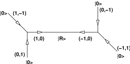
We begin by considering the case of the resolved conifold with the following web diagram. The operator at the right left vertex is S1superscript𝑆1S^{-1} which takes (01)matrix01\pmatrix{0\cr 1} to (10)matrix10\pmatrix{1\cr 0} and the operator at the right vertex is also S1superscript𝑆1S^{-1} since it takes (01)matrix01\pmatrix{0\cr-1} to (10)matrix10\pmatrix{-1\cr 0}. With vacuum states associated with the boundary circles at infinity we get the amplitude
Refer to caption
Figure 7: 5-brane web of the resolved conifold with vacuum states associated to the boundary circles.
Zconifoldsubscript𝑍𝑐𝑜𝑛𝑖𝑓𝑜𝑙𝑑\displaystyle Z_{conifold} =\displaystyle= R0,0|S1|RelRrR¯|S1|0,0,subscript𝑅quantum-operator-product00superscript𝑆1𝑅superscript𝑒subscript𝑙𝑅𝑟quantum-operator-product¯𝑅superscript𝑆100\displaystyle\sum_{R}\langle 0,0|S^{-1}|R\rangle e^{-l_{R}\,r}\langle\bar{R}|S^{-1}|0,0\rangle\,,
=\displaystyle= R0|S1|RelRrR¯|S1|0.subscript𝑅quantum-operator-product0superscript𝑆1𝑅superscript𝑒subscript𝑙𝑅𝑟quantum-operator-product¯𝑅superscript𝑆10\displaystyle\sum_{R}\langle 0|S^{-1}|R\rangle e^{-l_{R}\,r}\langle\bar{R}|S^{-1}|0\rangle\,.

We claim that the instanton corrections to the topological closed string amplitude on the resolved conifold Finst(c)subscriptsuperscript𝐹𝑐𝑖𝑛𝑠𝑡F^{(c)}_{inst} is given by

Finst(c)(T)=logZconifold(r),q=eigs.formulae-sequencesubscriptsuperscript𝐹𝑐𝑖𝑛𝑠𝑡𝑇logsubscript𝑍𝑐𝑜𝑛𝑖𝑓𝑜𝑙𝑑𝑟𝑞superscript𝑒𝑖subscript𝑔𝑠\displaystyle F^{(c)}_{inst}(T)=-\mbox{log}Z_{conifold}(r)\,,\,\,\,q=e^{ig_{s}}\,. (23)

Where T𝑇T is the renormalized Kähler parameter. Thus logZconifoldlogsubscript𝑍𝑐𝑜𝑛𝑖𝑓𝑜𝑙𝑑-\mbox{log}Z_{conifold} gives the instanton corrections to the closed topological string amplitude when written in terms of the renormalized Kähler parameter T𝑇T. To determine the relation between r𝑟r and T𝑇T we calculate the term proportional to ersuperscript𝑒𝑟e^{-r},

I1subscript𝐼1\displaystyle I_{1} =\displaystyle= er0|S1|RR¯|S1|0,superscript𝑒𝑟quantum-operator-product0superscript𝑆1𝑅quantum-operator-product¯𝑅superscript𝑆10\displaystyle e^{-r}\langle 0|S^{-1}|R\rangle\langle\bar{R}|S^{-1}|0\rangle\,,
=\displaystyle= erW 2,superscript𝑒𝑟subscriptsuperscript𝑊2 \displaystyle e^{-r}\,W^{2}_{\vbox{\offinterlineskip\kern 1.0pt\hbox{\kern 1.0pt\vbox{\hbox{\noindent\vbox{\hbox{\vbox to0.0pt{\hrule height=0.4pt,width=3.90555pt\vss}}\hbox{\vbox{\hbox to0.0pt{\vrule width=0.4pt,height=3.90555pt\hss}}\kern 3.90555pt\vbox{\hbox to0.0pt{\vrule width=0.4pt,height=3.90555pt\hss}}}\hbox{\vbox{\hbox{\vbox to0.0pt{\hrule height=0.4pt,width=4.30554pt\vss}}}\kern-0.4pt}}}\hbox{}}\kern 1.0pt\kern 0.4pt}\kern 1.0pt\kern 0.4pt}}\,,
=\displaystyle= er(λ1/2λ1/2q1/2q1/2)2.superscript𝑒𝑟superscriptsuperscript𝜆12superscript𝜆12superscript𝑞12superscript𝑞122\displaystyle e^{-r}\,(\frac{\lambda^{1/2}-\lambda^{-1/2}}{q^{1/2}-q^{-1/2}})^{2}\,.

In the large N𝑁N limit λmaps-to𝜆\lambda\mapsto\infty and therefore to get a finite non-vanishing result we define T𝑇T as follows

r=T+log(λ).𝑟𝑇log𝜆\displaystyle r=T+\mbox{log}(\lambda)\,. (25)

Then we can write Eq(4) as

eFinst(c)=RelRT𝒲R2(q).superscript𝑒subscriptsuperscript𝐹𝑐𝑖𝑛𝑠𝑡subscript𝑅superscript𝑒subscript𝑙𝑅𝑇subscriptsuperscript𝒲2𝑅𝑞\displaystyle e^{-F^{(c)}_{inst}}=\sum_{R}e^{-l_{R}T}\,{\cal W}^{2}_{R}(q)\,. (26)

Where as defined in the last section before 𝒲R(q)subscript𝒲𝑅𝑞{\cal W}_{R}(q) is the coefficient of λlR/2superscript𝜆subscript𝑙𝑅2\lambda^{l_{R}/2} in WR(q):=0|S1|Rassignsubscript𝑊𝑅𝑞quantum-operator-product0superscript𝑆1𝑅W_{R}(q):=\langle 0|S^{-1}|R\rangle. To see this gives the correct closed string expansion we calculate a few terms. Denoting the term proportional to enTsuperscript𝑒𝑛𝑇e^{-nT} by Insubscript𝐼𝑛I_{n} we have,

I1subscript𝐼1\displaystyle I_{1} :=assign\displaystyle:= eT𝒲 2=eT1(q1/2q1/2)2superscript𝑒𝑇subscriptsuperscript𝒲2 superscript𝑒𝑇1superscriptsuperscript𝑞12superscript𝑞122\displaystyle e^{-T}{\cal W}^{2}_{\vbox{\offinterlineskip\kern 1.0pt\hbox{\kern 1.0pt\vbox{\hbox{\noindent\vbox{\hbox{\vbox to0.0pt{\hrule height=0.4pt,width=3.90555pt\vss}}\hbox{\vbox{\hbox to0.0pt{\vrule width=0.4pt,height=3.90555pt\hss}}\kern 3.90555pt\vbox{\hbox to0.0pt{\vrule width=0.4pt,height=3.90555pt\hss}}}\hbox{\vbox{\hbox{\vbox to0.0pt{\hrule height=0.4pt,width=4.30554pt\vss}}}\kern-0.4pt}}}\hbox{}}\kern 1.0pt\kern 0.4pt}\kern 1.0pt\kern 0.4pt}}=e^{-T}\,\,\frac{1}{(q^{1/2}-q^{-1/2})^{2}} (27)
I2subscript𝐼2\displaystyle I_{2} :=assign\displaystyle:= e2T{𝒲 2+𝒲 2}=e2Tq+q1(q1/2q1/2)4(q1/2+q1/2)2,superscript𝑒2𝑇subscriptsuperscript𝒲2 subscriptsuperscript𝒲2 superscript𝑒2𝑇𝑞superscript𝑞1superscriptsuperscript𝑞12superscript𝑞124superscriptsuperscript𝑞12superscript𝑞122\displaystyle e^{-2T}\{{\cal W}^{2}_{\vbox{\offinterlineskip\kern 1.0pt\hbox{\kern 1.0pt\vbox{\hbox{\noindent\vbox{\hbox{\vbox to0.0pt{\hrule height=0.4pt,width=3.90555pt\vss}}\hbox{\vbox{\hbox to0.0pt{\vrule width=0.4pt,height=3.90555pt\hss}}\kern 3.90555pt\vbox{\hbox to0.0pt{\vrule width=0.4pt,height=3.90555pt\hss}}}\hbox{\vbox{\hbox{\vbox to0.0pt{\hrule height=0.4pt,width=4.30554pt\vss}}}\kern-0.4pt}}\vbox{\hbox{\vbox to0.0pt{\hrule height=0.4pt,width=3.90555pt\vss}}\hbox{\vbox{\hbox to0.0pt{\vrule width=0.4pt,height=3.90555pt\hss}}\kern 3.90555pt\vbox{\hbox to0.0pt{\vrule width=0.4pt,height=3.90555pt\hss}}}\hbox{\vbox{\hbox{\vbox to0.0pt{\hrule height=0.4pt,width=4.30554pt\vss}}}\kern-0.4pt}}}\hbox{}}\kern 1.0pt\kern 0.4pt}\kern 1.0pt\kern 0.4pt}}+{\cal W}^{2}_{\vbox{\offinterlineskip\kern 1.0pt\hbox{\kern 1.0pt\vbox{\hbox{\noindent\vbox{\hbox{\vbox to0.0pt{\hrule height=0.4pt,width=3.90555pt\vss}}\hbox{\vbox{\hbox to0.0pt{\vrule width=0.4pt,height=3.90555pt\hss}}\kern 3.90555pt\vbox{\hbox to0.0pt{\vrule width=0.4pt,height=3.90555pt\hss}}}\hbox{\vbox{\hbox{\vbox to0.0pt{\hrule height=0.4pt,width=4.30554pt\vss}}}\kern-0.4pt}}}\hbox{\noindent\vbox{\hbox{\vbox to0.0pt{\hrule height=0.4pt,width=3.90555pt\vss}}\hbox{\vbox{\hbox to0.0pt{\vrule width=0.4pt,height=3.90555pt\hss}}\kern 3.90555pt\vbox{\hbox to0.0pt{\vrule width=0.4pt,height=3.90555pt\hss}}}\hbox{\vbox{\hbox{\vbox to0.0pt{\hrule height=0.4pt,width=4.30554pt\vss}}}\kern-0.4pt}}}\hbox{}}\kern 1.0pt\kern 0.4pt}\kern 1.0pt\kern 0.4pt}}\}=e^{-2T}\,\,\frac{q+q^{-1}}{(q^{1/2}-q^{-1/2})^{4}(q^{1/2}+q^{-1/2})^{2}}\,,
I3subscript𝐼3\displaystyle I_{3} :=assign\displaystyle:= e3T{𝒲 2+𝒲 2+𝒲 2}=e3T(q3+q3)+(q+q1)+2(q1/2q1/2)4(q1/2+q1/2)2(q3/2q3/2)2,superscript𝑒3𝑇subscriptsuperscript𝒲2 subscriptsuperscript𝒲2 subscriptsuperscript𝒲2 superscript𝑒3𝑇superscript𝑞3superscript𝑞3𝑞superscript𝑞12superscriptsuperscript𝑞12superscript𝑞124superscriptsuperscript𝑞12superscript𝑞122superscriptsuperscript𝑞32superscript𝑞322\displaystyle e^{-3T}\{{\cal W}^{2}_{\vbox{\offinterlineskip\kern 1.0pt\hbox{\kern 1.0pt\vbox{\hbox{\noindent\vbox{\hbox{\vbox to0.0pt{\hrule height=0.4pt,width=3.90555pt\vss}}\hbox{\vbox{\hbox to0.0pt{\vrule width=0.4pt,height=3.90555pt\hss}}\kern 3.90555pt\vbox{\hbox to0.0pt{\vrule width=0.4pt,height=3.90555pt\hss}}}\hbox{\vbox{\hbox{\vbox to0.0pt{\hrule height=0.4pt,width=4.30554pt\vss}}}\kern-0.4pt}}\vbox{\hbox{\vbox to0.0pt{\hrule height=0.4pt,width=3.90555pt\vss}}\hbox{\vbox{\hbox to0.0pt{\vrule width=0.4pt,height=3.90555pt\hss}}\kern 3.90555pt\vbox{\hbox to0.0pt{\vrule width=0.4pt,height=3.90555pt\hss}}}\hbox{\vbox{\hbox{\vbox to0.0pt{\hrule height=0.4pt,width=4.30554pt\vss}}}\kern-0.4pt}}\vbox{\hbox{\vbox to0.0pt{\hrule height=0.4pt,width=3.90555pt\vss}}\hbox{\vbox{\hbox to0.0pt{\vrule width=0.4pt,height=3.90555pt\hss}}\kern 3.90555pt\vbox{\hbox to0.0pt{\vrule width=0.4pt,height=3.90555pt\hss}}}\hbox{\vbox{\hbox{\vbox to0.0pt{\hrule height=0.4pt,width=4.30554pt\vss}}}\kern-0.4pt}}}\hbox{}}\kern 1.0pt\kern 0.4pt}\kern 1.0pt\kern 0.4pt}}+{\cal W}^{2}_{\vbox{\offinterlineskip\kern 1.0pt\hbox{\kern 1.0pt\vbox{\hbox{\noindent\vbox{\hbox{\vbox to0.0pt{\hrule height=0.4pt,width=3.90555pt\vss}}\hbox{\vbox{\hbox to0.0pt{\vrule width=0.4pt,height=3.90555pt\hss}}\kern 3.90555pt\vbox{\hbox to0.0pt{\vrule width=0.4pt,height=3.90555pt\hss}}}\hbox{\vbox{\hbox{\vbox to0.0pt{\hrule height=0.4pt,width=4.30554pt\vss}}}\kern-0.4pt}}\vbox{\hbox{\vbox to0.0pt{\hrule height=0.4pt,width=3.90555pt\vss}}\hbox{\vbox{\hbox to0.0pt{\vrule width=0.4pt,height=3.90555pt\hss}}\kern 3.90555pt\vbox{\hbox to0.0pt{\vrule width=0.4pt,height=3.90555pt\hss}}}\hbox{\vbox{\hbox{\vbox to0.0pt{\hrule height=0.4pt,width=4.30554pt\vss}}}\kern-0.4pt}}}\hbox{\noindent\vbox{\hbox{\vbox to0.0pt{\hrule height=0.4pt,width=3.90555pt\vss}}\hbox{\vbox{\hbox to0.0pt{\vrule width=0.4pt,height=3.90555pt\hss}}\kern 3.90555pt\vbox{\hbox to0.0pt{\vrule width=0.4pt,height=3.90555pt\hss}}}\hbox{\vbox{\hbox{\vbox to0.0pt{\hrule height=0.4pt,width=4.30554pt\vss}}}\kern-0.4pt}}}\hbox{}}\kern 1.0pt\kern 0.4pt}\kern 1.0pt\kern 0.4pt}}+{\cal W}^{2}_{\vbox{\offinterlineskip\kern 1.0pt\hbox{\kern 1.0pt\vbox{\hbox{\noindent\vbox{\hbox{\vbox to0.0pt{\hrule height=0.4pt,width=3.90555pt\vss}}\hbox{\vbox{\hbox to0.0pt{\vrule width=0.4pt,height=3.90555pt\hss}}\kern 3.90555pt\vbox{\hbox to0.0pt{\vrule width=0.4pt,height=3.90555pt\hss}}}\hbox{\vbox{\hbox{\vbox to0.0pt{\hrule height=0.4pt,width=4.30554pt\vss}}}\kern-0.4pt}}}\hbox{\noindent\vbox{\hbox{\vbox to0.0pt{\hrule height=0.4pt,width=3.90555pt\vss}}\hbox{\vbox{\hbox to0.0pt{\vrule width=0.4pt,height=3.90555pt\hss}}\kern 3.90555pt\vbox{\hbox to0.0pt{\vrule width=0.4pt,height=3.90555pt\hss}}}\hbox{\vbox{\hbox{\vbox to0.0pt{\hrule height=0.4pt,width=4.30554pt\vss}}}\kern-0.4pt}}}\hbox{\noindent\vbox{\hbox{\vbox to0.0pt{\hrule height=0.4pt,width=3.90555pt\vss}}\hbox{\vbox{\hbox to0.0pt{\vrule width=0.4pt,height=3.90555pt\hss}}\kern 3.90555pt\vbox{\hbox to0.0pt{\vrule width=0.4pt,height=3.90555pt\hss}}}\hbox{\vbox{\hbox{\vbox to0.0pt{\hrule height=0.4pt,width=4.30554pt\vss}}}\kern-0.4pt}}}\hbox{}}\kern 1.0pt\kern 0.4pt}\kern 1.0pt\kern 0.4pt}}\}=e^{-3T}\frac{(q^{3}+q^{-3})+(q+q^{-1})+2}{(q^{1/2}-q^{-1/2})^{4}(q^{1/2}+q^{-1/2})^{2}(q^{3/2}-q^{-3/2})^{2}}\,,
I4subscript𝐼4\displaystyle I_{4} :=assign\displaystyle:= e4T{𝒲 2+𝒲 2+𝒲 2+𝒲 2+𝒲 2}superscript𝑒4𝑇subscriptsuperscript𝒲2 subscriptsuperscript𝒲2 subscriptsuperscript𝒲2 subscriptsuperscript𝒲2 subscriptsuperscript𝒲2 \displaystyle e^{-4T}\{{\cal W}^{2}_{\vbox{\offinterlineskip\kern 1.0pt\hbox{\kern 1.0pt\vbox{\hbox{\noindent\vbox{\hbox{\vbox to0.0pt{\hrule height=0.4pt,width=3.90555pt\vss}}\hbox{\vbox{\hbox to0.0pt{\vrule width=0.4pt,height=3.90555pt\hss}}\kern 3.90555pt\vbox{\hbox to0.0pt{\vrule width=0.4pt,height=3.90555pt\hss}}}\hbox{\vbox{\hbox{\vbox to0.0pt{\hrule height=0.4pt,width=4.30554pt\vss}}}\kern-0.4pt}}\vbox{\hbox{\vbox to0.0pt{\hrule height=0.4pt,width=3.90555pt\vss}}\hbox{\vbox{\hbox to0.0pt{\vrule width=0.4pt,height=3.90555pt\hss}}\kern 3.90555pt\vbox{\hbox to0.0pt{\vrule width=0.4pt,height=3.90555pt\hss}}}\hbox{\vbox{\hbox{\vbox to0.0pt{\hrule height=0.4pt,width=4.30554pt\vss}}}\kern-0.4pt}}\vbox{\hbox{\vbox to0.0pt{\hrule height=0.4pt,width=3.90555pt\vss}}\hbox{\vbox{\hbox to0.0pt{\vrule width=0.4pt,height=3.90555pt\hss}}\kern 3.90555pt\vbox{\hbox to0.0pt{\vrule width=0.4pt,height=3.90555pt\hss}}}\hbox{\vbox{\hbox{\vbox to0.0pt{\hrule height=0.4pt,width=4.30554pt\vss}}}\kern-0.4pt}}\vbox{\hbox{\vbox to0.0pt{\hrule height=0.4pt,width=3.90555pt\vss}}\hbox{\vbox{\hbox to0.0pt{\vrule width=0.4pt,height=3.90555pt\hss}}\kern 3.90555pt\vbox{\hbox to0.0pt{\vrule width=0.4pt,height=3.90555pt\hss}}}\hbox{\vbox{\hbox{\vbox to0.0pt{\hrule height=0.4pt,width=4.30554pt\vss}}}\kern-0.4pt}}}\hbox{}}\kern 1.0pt\kern 0.4pt}\kern 1.0pt\kern 0.4pt}}+{\cal W}^{2}_{\vbox{\offinterlineskip\kern 1.0pt\hbox{\kern 1.0pt\vbox{\hbox{\noindent\vbox{\hbox{\vbox to0.0pt{\hrule height=0.4pt,width=3.90555pt\vss}}\hbox{\vbox{\hbox to0.0pt{\vrule width=0.4pt,height=3.90555pt\hss}}\kern 3.90555pt\vbox{\hbox to0.0pt{\vrule width=0.4pt,height=3.90555pt\hss}}}\hbox{\vbox{\hbox{\vbox to0.0pt{\hrule height=0.4pt,width=4.30554pt\vss}}}\kern-0.4pt}}\vbox{\hbox{\vbox to0.0pt{\hrule height=0.4pt,width=3.90555pt\vss}}\hbox{\vbox{\hbox to0.0pt{\vrule width=0.4pt,height=3.90555pt\hss}}\kern 3.90555pt\vbox{\hbox to0.0pt{\vrule width=0.4pt,height=3.90555pt\hss}}}\hbox{\vbox{\hbox{\vbox to0.0pt{\hrule height=0.4pt,width=4.30554pt\vss}}}\kern-0.4pt}}\vbox{\hbox{\vbox to0.0pt{\hrule height=0.4pt,width=3.90555pt\vss}}\hbox{\vbox{\hbox to0.0pt{\vrule width=0.4pt,height=3.90555pt\hss}}\kern 3.90555pt\vbox{\hbox to0.0pt{\vrule width=0.4pt,height=3.90555pt\hss}}}\hbox{\vbox{\hbox{\vbox to0.0pt{\hrule height=0.4pt,width=4.30554pt\vss}}}\kern-0.4pt}}}\hbox{\noindent\vbox{\hbox{\vbox to0.0pt{\hrule height=0.4pt,width=3.90555pt\vss}}\hbox{\vbox{\hbox to0.0pt{\vrule width=0.4pt,height=3.90555pt\hss}}\kern 3.90555pt\vbox{\hbox to0.0pt{\vrule width=0.4pt,height=3.90555pt\hss}}}\hbox{\vbox{\hbox{\vbox to0.0pt{\hrule height=0.4pt,width=4.30554pt\vss}}}\kern-0.4pt}}}\hbox{}}\kern 1.0pt\kern 0.4pt}\kern 1.0pt\kern 0.4pt}}+{\cal W}^{2}_{\vbox{\offinterlineskip\kern 1.0pt\hbox{\kern 1.0pt\vbox{\hbox{\noindent\vbox{\hbox{\vbox to0.0pt{\hrule height=0.4pt,width=3.90555pt\vss}}\hbox{\vbox{\hbox to0.0pt{\vrule width=0.4pt,height=3.90555pt\hss}}\kern 3.90555pt\vbox{\hbox to0.0pt{\vrule width=0.4pt,height=3.90555pt\hss}}}\hbox{\vbox{\hbox{\vbox to0.0pt{\hrule height=0.4pt,width=4.30554pt\vss}}}\kern-0.4pt}}\vbox{\hbox{\vbox to0.0pt{\hrule height=0.4pt,width=3.90555pt\vss}}\hbox{\vbox{\hbox to0.0pt{\vrule width=0.4pt,height=3.90555pt\hss}}\kern 3.90555pt\vbox{\hbox to0.0pt{\vrule width=0.4pt,height=3.90555pt\hss}}}\hbox{\vbox{\hbox{\vbox to0.0pt{\hrule height=0.4pt,width=4.30554pt\vss}}}\kern-0.4pt}}}\hbox{\noindent\vbox{\hbox{\vbox to0.0pt{\hrule height=0.4pt,width=3.90555pt\vss}}\hbox{\vbox{\hbox to0.0pt{\vrule width=0.4pt,height=3.90555pt\hss}}\kern 3.90555pt\vbox{\hbox to0.0pt{\vrule width=0.4pt,height=3.90555pt\hss}}}\hbox{\vbox{\hbox{\vbox to0.0pt{\hrule height=0.4pt,width=4.30554pt\vss}}}\kern-0.4pt}}\vbox{\hbox{\vbox to0.0pt{\hrule height=0.4pt,width=3.90555pt\vss}}\hbox{\vbox{\hbox to0.0pt{\vrule width=0.4pt,height=3.90555pt\hss}}\kern 3.90555pt\vbox{\hbox to0.0pt{\vrule width=0.4pt,height=3.90555pt\hss}}}\hbox{\vbox{\hbox{\vbox to0.0pt{\hrule height=0.4pt,width=4.30554pt\vss}}}\kern-0.4pt}}}\hbox{}}\kern 1.0pt\kern 0.4pt}\kern 1.0pt\kern 0.4pt}}+{\cal W}^{2}_{\vbox{\offinterlineskip\kern 1.0pt\hbox{\kern 1.0pt\vbox{\hbox{\noindent\vbox{\hbox{\vbox to0.0pt{\hrule height=0.4pt,width=3.90555pt\vss}}\hbox{\vbox{\hbox to0.0pt{\vrule width=0.4pt,height=3.90555pt\hss}}\kern 3.90555pt\vbox{\hbox to0.0pt{\vrule width=0.4pt,height=3.90555pt\hss}}}\hbox{\vbox{\hbox{\vbox to0.0pt{\hrule height=0.4pt,width=4.30554pt\vss}}}\kern-0.4pt}}\vbox{\hbox{\vbox to0.0pt{\hrule height=0.4pt,width=3.90555pt\vss}}\hbox{\vbox{\hbox to0.0pt{\vrule width=0.4pt,height=3.90555pt\hss}}\kern 3.90555pt\vbox{\hbox to0.0pt{\vrule width=0.4pt,height=3.90555pt\hss}}}\hbox{\vbox{\hbox{\vbox to0.0pt{\hrule height=0.4pt,width=4.30554pt\vss}}}\kern-0.4pt}}}\hbox{\noindent\vbox{\hbox{\vbox to0.0pt{\hrule height=0.4pt,width=3.90555pt\vss}}\hbox{\vbox{\hbox to0.0pt{\vrule width=0.4pt,height=3.90555pt\hss}}\kern 3.90555pt\vbox{\hbox to0.0pt{\vrule width=0.4pt,height=3.90555pt\hss}}}\hbox{\vbox{\hbox{\vbox to0.0pt{\hrule height=0.4pt,width=4.30554pt\vss}}}\kern-0.4pt}}}\hbox{\noindent\vbox{\hbox{\vbox to0.0pt{\hrule height=0.4pt,width=3.90555pt\vss}}\hbox{\vbox{\hbox to0.0pt{\vrule width=0.4pt,height=3.90555pt\hss}}\kern 3.90555pt\vbox{\hbox to0.0pt{\vrule width=0.4pt,height=3.90555pt\hss}}}\hbox{\vbox{\hbox{\vbox to0.0pt{\hrule height=0.4pt,width=4.30554pt\vss}}}\kern-0.4pt}}}\hbox{}}\kern 1.0pt\kern 0.4pt}\kern 1.0pt\kern 0.4pt}}+{\cal W}^{2}_{\vbox{\offinterlineskip\kern 1.0pt\hbox{\kern 1.0pt\vbox{\hbox{\noindent\vbox{\hbox{\vbox to0.0pt{\hrule height=0.4pt,width=3.90555pt\vss}}\hbox{\vbox{\hbox to0.0pt{\vrule width=0.4pt,height=3.90555pt\hss}}\kern 3.90555pt\vbox{\hbox to0.0pt{\vrule width=0.4pt,height=3.90555pt\hss}}}\hbox{\vbox{\hbox{\vbox to0.0pt{\hrule height=0.4pt,width=4.30554pt\vss}}}\kern-0.4pt}}}\hbox{\noindent\vbox{\hbox{\vbox to0.0pt{\hrule height=0.4pt,width=3.90555pt\vss}}\hbox{\vbox{\hbox to0.0pt{\vrule width=0.4pt,height=3.90555pt\hss}}\kern 3.90555pt\vbox{\hbox to0.0pt{\vrule width=0.4pt,height=3.90555pt\hss}}}\hbox{\vbox{\hbox{\vbox to0.0pt{\hrule height=0.4pt,width=4.30554pt\vss}}}\kern-0.4pt}}}\hbox{\noindent\vbox{\hbox{\vbox to0.0pt{\hrule height=0.4pt,width=3.90555pt\vss}}\hbox{\vbox{\hbox to0.0pt{\vrule width=0.4pt,height=3.90555pt\hss}}\kern 3.90555pt\vbox{\hbox to0.0pt{\vrule width=0.4pt,height=3.90555pt\hss}}}\hbox{\vbox{\hbox{\vbox to0.0pt{\hrule height=0.4pt,width=4.30554pt\vss}}}\kern-0.4pt}}}\hbox{\noindent\vbox{\hbox{\vbox to0.0pt{\hrule height=0.4pt,width=3.90555pt\vss}}\hbox{\vbox{\hbox to0.0pt{\vrule width=0.4pt,height=3.90555pt\hss}}\kern 3.90555pt\vbox{\hbox to0.0pt{\vrule width=0.4pt,height=3.90555pt\hss}}}\hbox{\vbox{\hbox{\vbox to0.0pt{\hrule height=0.4pt,width=4.30554pt\vss}}}\kern-0.4pt}}}\hbox{}}\kern 1.0pt\kern 0.4pt}\kern 1.0pt\kern 0.4pt}}\}
=\displaystyle= e4TC(q)(q1/2q1/2)6(q1/2+q1/2)4(q+q1)2(q3/2q3/2)2.superscript𝑒4𝑇𝐶𝑞superscriptsuperscript𝑞12superscript𝑞126superscriptsuperscript𝑞12superscript𝑞124superscript𝑞superscript𝑞12superscriptsuperscript𝑞32superscript𝑞322\displaystyle e^{-4T}\frac{C(q)}{(q^{1/2}-q^{-1/2})^{6}(q^{1/2}+q^{-1/2})^{4}(q+q^{-1})^{2}(q^{3/2}-q^{-3/2})^{2}}\,.

Where

C(q):=(q6+q6)+(q4+q4)+2(q3+q3)+4(q2+q2)+2(q+q1)+4.assign𝐶𝑞superscript𝑞6superscript𝑞6superscript𝑞4superscript𝑞42superscript𝑞3superscript𝑞34superscript𝑞2superscript𝑞22𝑞superscript𝑞14\displaystyle C(q):=(q^{6}+q^{-6})+(q^{4}+q^{-4})+2(q^{3}+q^{-3})+4(q^{2}+q^{-2})+2(q+q^{-1})+4\,. (28)

Since the resolved conifold has a single IP1IsuperscriptP1\mbox{I}\!\mbox{P}^{1} from Eq(1) it follows that the closed string expansion for the conifold is given by [10]

Finst(c)(T)=n=1g=0NCgn(2sin(ngs/2))2g2enT.subscriptsuperscript𝐹𝑐𝑖𝑛𝑠𝑡𝑇superscriptsubscript𝑛1superscriptsubscript𝑔0subscriptsuperscript𝑁𝑔𝐶𝑛superscript2sin𝑛subscript𝑔𝑠22𝑔2superscript𝑒𝑛𝑇\displaystyle F^{(c)}_{inst}(T)=\sum_{n=1}^{\infty}\sum_{g=0}^{\infty}\frac{N^{g}_{C}}{n}(2\mbox{sin}(ng_{s}/2))^{2g-2}\,e^{-nT}\,. (29)

Comparing this with Eq(26) using Eq(27) we get

logZconifoldlogsubscript𝑍𝑐𝑜𝑛𝑖𝑓𝑜𝑙𝑑\displaystyle-\mbox{log}Z_{conifold} =\displaystyle= log(1+I1+I2+I3+I4+),log1subscript𝐼1subscript𝐼2subscript𝐼3subscript𝐼4\displaystyle\mbox{log}(1+I_{1}+I_{2}+I_{3}+I_{4}+\cdots)\,,
=\displaystyle= I1+{I212I12}+{I3I2I1+13I13}+{I4I3I1+I2I1212I2214I14}+,subscript𝐼1subscript𝐼212superscriptsubscript𝐼12subscript𝐼3subscript𝐼2subscript𝐼113superscriptsubscript𝐼13subscript𝐼4subscript𝐼3subscript𝐼1subscript𝐼2superscriptsubscript𝐼1212superscriptsubscript𝐼2214superscriptsubscript𝐼14\displaystyle I_{1}+\{I_{2}-\frac{1}{2}I_{1}^{2}\}+\{I_{3}-I_{2}I_{1}+\frac{1}{3}I_{1}^{3}\}+\{I_{4}-I_{3}I_{1}+I_{2}I_{1}^{2}-\frac{1}{2}I_{2}^{2}-\frac{1}{4}I_{1}^{4}\}+\cdots\,,
=\displaystyle= eT(2sin(gs/2))2+e2T2(2sin(gs))2+e3T3(2sin(3gs/2))2+e4T4(2sin(2gs))2+.superscript𝑒𝑇superscript2sinsubscript𝑔𝑠22superscript𝑒2𝑇2superscript2sinsubscript𝑔𝑠2superscript𝑒3𝑇3superscript2sin3subscript𝑔𝑠22superscript𝑒4𝑇4superscript2sin2subscript𝑔𝑠2\displaystyle\frac{e^{-T}}{(2\mbox{sin}(g_{s}/2))^{2}}+\frac{e^{-2T}}{2(2\mbox{sin}(g_{s}))^{2}}+\frac{e^{-3T}}{3(2\mbox{sin}(3g_{s}/2))^{2}}+\frac{e^{-4T}}{4(2\mbox{sin}(2g_{s}))^{2}}+\cdots\,.

Which agrees with the expected closed string expansion.

5 Calabi-Yau with single compact divisor

In this section we will discuss non-compact toric Calabi-Yau threefolds which have a single compact divisor. These Calabi-Yau manifolds are the total space of the canonical line bundle over a toric Fano or toric almost Fano surface. We will consider the case of blowups of IP2IsuperscriptP2\mbox{I}\!\mbox{P}^{2} and the blowups of first and second Hirzebruch surfaces. We denote the blow up of IP2IsuperscriptP2\mbox{I}\!\mbox{P}^{2} at k𝑘k points by ksubscript𝑘{\cal B}_{k}.

Refer to caption
Figure 8: a) IP2IsuperscriptP2\mbox{I}\!\mbox{P}^{2},   b)1subscript1{\cal B}_{1},   c)2subscript2{\cal B}_{2},   d)3subscript3{\cal B}_{3},   e) IP1×IP1IsuperscriptP1IsuperscriptP1\mbox{I}\!\mbox{P}^{1}\times\mbox{I}\!\mbox{P}^{1},   f) F2subscript𝐹2F_{2}, g) F2subscript𝐹2F_{2} blown up at one point,   h) F2subscript𝐹2F_{2} blown up at two points.

5.1 IP2IsuperscriptP2\mbox{I}\!\mbox{P}^{2}

The amplitude associated with the web diagram can be written down completely once the gluing matrices associated with each vertex are known. All Riemann surfaces corresponding to the 5-brane webs can be constructed from a ”propagator” (a cylinder) and SL(2,𝖹𝖹)𝑆𝐿2𝖹𝖹SL(2,{\sf Z\!\!\!Z}) transform of a ”three point vertex” ( a sphere with three disks removed). The SL(2,𝖹𝖹)𝑆𝐿2𝖹𝖹SL(2,{\sf Z\!\!\!Z}) gluing matrices associated with the vertices of the brane web contain the information about how the propagators and the three point vertex are to be put together to get the web. These gluing matrices are SL(2,𝖹𝖹)𝑆𝐿2𝖹𝖹SL(2,{\sf Z\!\!\!Z}) matrices which transform one edge of the three point vertex with charge (p,q)𝑝𝑞(p,q) into another edge with charge (r,s)𝑟𝑠(r,s). For the case of non-compact Calabi-Yaus with a single compact divisor the Riemann surface is of genus one which is reflected by the fact that the 5-brane web has a single “face”. In this case we see that each three point vertex used to construct the web has two edges which are the internal edges and therefore it is natural to define the gluing matrix at that vertex to be the SL(2,𝖹𝖹)𝑆𝐿2𝖹𝖹SL(2,{\sf Z\!\!\!Z}) matrix which maps one internal edge to another internal edge associated with that vertex consistent with the vertex defined before.

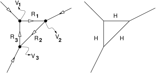
We begin with the case of IP2IsuperscriptP2\mbox{I}\!\mbox{P}^{2}, which was discussed in detail in [21], for completeness. The non-compact Calabi-Yau manifold is the total space of 𝒪(3)𝒪3{\cal O}(-3) bundle over IP2IsuperscriptP2\mbox{I}\!\mbox{P}^{2}. The web diagram dual to this non-compact CY can be obtained from the toric diagrams given in Fig. 8(a) and is shown in Fig. 9.
Refer to caption
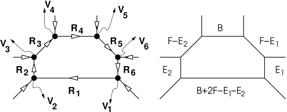
Figure 9: a) The 5-brane web dual to the local IP2IsuperscriptP2\mbox{I}\!\mbox{P}^{2}, (p,q)𝑝𝑞(p,q) 5-brane is oriented in the direction (p,q)𝑝𝑞(p,q). Rasubscript𝑅𝑎R_{a} denote the states propagating on the internal lines, b) the rational curve classes of the internal edges.

The equation for the Riemann surface which gives the dual theory when M5-brane is wrapped on it can be easily determined from the mirror superpotential or the toric data [29, 30]

1+eu+ev+etuv=0.1superscript𝑒𝑢superscript𝑒𝑣superscript𝑒𝑡𝑢𝑣0\displaystyle 1+e^{u}+e^{v}+e^{-t-u-v}=0\,. (31)

Where t𝑡t is the Kähler parameter of the generator of H2(IP2,𝖹𝖹)subscript𝐻2IsuperscriptP2𝖹𝖹H_{2}(\mbox{I}\!\mbox{P}^{2},{\sf Z\!\!\!Z}) which we will denote by H𝐻H. H𝐻H is the class of IP1IsuperscriptP1\mbox{I}\!\mbox{P}^{1} given by a linear equation in IP2IsuperscriptP2\mbox{I}\!\mbox{P}^{2} and is such that HH=1𝐻𝐻1H\cdot H=1. From the web digram we can determine the operators associated with the vertices. These operators are just the operators in the WZW theory corresponding to the SL(2,𝖹𝖹)𝑆𝐿2𝖹𝖹SL(2,{\sf Z\!\!\!Z}) matrices mapping the internal edges into each other at each vertex,

(01)𝒱1(10)𝒱2(11)𝒱3(01),superscriptmaps-tosubscript𝒱1matrix01matrix10superscriptmaps-tosubscript𝒱2matrix11superscriptmaps-tosubscript𝒱3matrix01\displaystyle\pmatrix{0\cr 1}\stackrel{{\scriptstyle{\cal V}_{1}}}{{\mapsto}}\pmatrix{1\cr 0}\stackrel{{\scriptstyle{\cal V}_{2}}}{{\mapsto}}\pmatrix{-1\cr-1}\stackrel{{\scriptstyle{\cal V}_{3}}}{{\mapsto}}\pmatrix{0\cr 1}\,, (32)
𝒱1=S1,𝒱2=TS1T,𝒱3=TS1.formulae-sequencesubscript𝒱1superscript𝑆1formulae-sequencesubscript𝒱2𝑇superscript𝑆1𝑇subscript𝒱3𝑇superscript𝑆1\displaystyle{\cal V}_{1}=S^{-1}\,,\,\,{\cal V}_{2}=TS^{-1}T\,,\,\,{\cal V}_{3}=TS^{-1}\,.

Given these operators associated with the vertices we can write down the instanton contribution to the closed string amplitude (this can also be obtained as the large N limit of the Chern-Simons theory on local B3subscript𝐵3B_{3} with three non intersecting exceptional curves geometrically transitioned to S3superscript𝑆3S^{3} as was done in[21]),

eFinst(c)superscript𝑒subscriptsuperscript𝐹𝑐𝑖𝑛𝑠𝑡\displaystyle e^{F^{(c)}_{inst}} =\displaystyle= R1,R2,R3ea=13laraR3¯|𝒱3|R2,0R2¯|𝒱2|R1,0R1¯|𝒱1|R3,0,subscriptsubscript𝑅1subscript𝑅2subscript𝑅3superscript𝑒superscriptsubscript𝑎13subscript𝑙𝑎subscript𝑟𝑎quantum-operator-product¯subscript𝑅3subscript𝒱3subscript𝑅20quantum-operator-product¯subscript𝑅2subscript𝒱2subscript𝑅10quantum-operator-product¯subscript𝑅1subscript𝒱1subscript𝑅30\displaystyle\sum_{R_{1},R_{2},R_{3}}e^{-\sum_{a=1}^{3}l_{a}r_{a}}\langle\bar{R_{3}}|{\cal V}_{3}|R_{2},0\rangle\langle\bar{R_{2}}|{\cal V}_{2}|R_{1},0\rangle\langle\bar{R_{1}}|{\cal V}_{1}|R_{3},0\rangle\,,
=\displaystyle= R1,R2,R3ea=13laraR3¯|𝒱3|R2R2¯|𝒱2|R1R1¯|𝒱1|R3.subscriptsubscript𝑅1subscript𝑅2subscript𝑅3superscript𝑒superscriptsubscript𝑎13subscript𝑙𝑎subscript𝑟𝑎quantum-operator-product¯subscript𝑅3subscript𝒱3subscript𝑅2quantum-operator-product¯subscript𝑅2subscript𝒱2subscript𝑅1quantum-operator-product¯subscript𝑅1subscript𝒱1subscript𝑅3\displaystyle\sum_{R_{1},R_{2},R_{3}}e^{-\sum_{a=1}^{3}l_{a}r_{a}}\langle\bar{R_{3}}|{\cal V}_{3}|R_{2}\rangle\langle\bar{R_{2}}|{\cal V}_{2}|R_{1}\rangle\langle\bar{R_{1}}|{\cal V}_{1}|R_{3}\rangle\,.

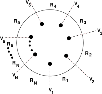
Note: Local IP2IsuperscriptP2\mbox{I}\!\mbox{P}^{2} blown up at more than three points have web diagrams in which some of the external legs are either parallel or cross each other. This is due to the fact that IP2IsuperscriptP2\mbox{I}\!\mbox{P}^{2} blown up at more than three points in not toric although we can choose special points and blow them up. The problem of intersecting external legs was solved in [24] by placing appropriate (p,q)7-brane and allowing the 5-brane to end on these 7-brane so that the external 5-brane no longer can go to infinity and cross each other. This 5-brane/7-brane picture can be simplified so that the web is given by a single 5-brane going around the 7-brane as shown in Fig. 10 below.
Refer to caption
Figure 10: 5-brane/7-brane description of toric and non-toric local Calabi-Yau’s.

In this picture it is easy to generalize and write amplitudes for non-toric local Calabi-Yau,

eFinst(c):=a=1NRaei=1Nlirii=1NRi+1|𝒱i+1|Ri.assignsuperscript𝑒subscriptsuperscript𝐹𝑐𝑖𝑛𝑠𝑡superscriptsubscript𝑎1𝑁subscriptsubscript𝑅𝑎superscript𝑒superscriptsubscript𝑖1𝑁subscript𝑙𝑖subscript𝑟𝑖superscriptsubscriptproduct𝑖1𝑁quantum-operator-productsubscript𝑅𝑖1subscript𝒱𝑖1subscript𝑅𝑖\displaystyle e^{F^{(c)}_{inst}}:=\sum_{a=1}^{N}\sum_{R_{a}}e^{-\sum_{i=1}^{N}l_{i}r_{i}}\prod_{i=1}^{N}\langle R_{i+1}|{\cal V}_{i+1}|R_{i}\rangle\,. (34)

Where 𝒱isubscript𝒱𝑖{\cal V}_{i} are the SL(2,𝖹𝖹)𝑆𝐿2𝖹𝖹SL(2,{\sf Z\!\!\!Z}) monodromy matrices associated with the 7-branes. These amplitudes for non-toric Calabi-Yau spaces will be discussed elsewhere [18].

Coming back to the local IP2IsuperscriptP2\mbox{I}\!\mbox{P}^{2} case we determine the relation between rasubscript𝑟𝑎r_{a} and the renormalized Kähler parameter by calculating the terms with only one non-vanishing lasubscript𝑙𝑎l_{a}.

la=δabsubscript𝑙𝑎subscript𝛿𝑎𝑏l_{a}=\delta_{ab}: We denote the term with la=δabsubscript𝑙𝑎subscript𝛿𝑎𝑏l_{a}=\delta_{ab} by bsubscript𝑏{\cal I}_{b},

bsubscript𝑏\displaystyle{\cal I}_{b} =\displaystyle= erb(1)W, 2(λ,q),superscript𝑒subscript𝑟𝑏1subscriptsuperscript𝑊2 𝜆𝑞\displaystyle e^{-r_{b}}(-1)W^{2}_{\cdot,\vbox{\offinterlineskip\kern 1.0pt\hbox{\kern 1.0pt\vbox{\hbox{\noindent\vbox{\hbox{\vbox to0.0pt{\hrule height=0.4pt,width=3.90555pt\vss}}\hbox{\vbox{\hbox to0.0pt{\vrule width=0.4pt,height=3.90555pt\hss}}\kern 3.90555pt\vbox{\hbox to0.0pt{\vrule width=0.4pt,height=3.90555pt\hss}}}\hbox{\vbox{\hbox{\vbox to0.0pt{\hrule height=0.4pt,width=4.30554pt\vss}}}\kern-0.4pt}}}\hbox{}}\kern 1.0pt\kern 0.4pt}\kern 1.0pt\kern 0.4pt}}(\lambda,q)\,,
=\displaystyle= erb(λ1/2λ1/2q1/2q1/2)2,superscript𝑒subscript𝑟𝑏superscriptsuperscript𝜆12superscript𝜆12superscript𝑞12superscript𝑞122\displaystyle-e^{-r_{b}}(\frac{\lambda^{1/2}-\lambda^{-1/2}}{q^{1/2}-q^{-1/2}})^{2}\,,
=\displaystyle= eTb(q1/2q1/2)2,superscript𝑒subscript𝑇𝑏superscriptsuperscript𝑞12superscript𝑞122\displaystyle-\frac{e^{-T_{b}}}{(q^{1/2}-q^{-1/2})^{2}}\,,
=\displaystyle= eTb(2sin(gs/2))2.superscript𝑒subscript𝑇𝑏superscript2sinsubscript𝑔𝑠22\displaystyle\frac{e^{-T_{b}}}{(2\mbox{sin}(g_{s}/2))^{2}}\,.

Where the minus sign comes from the action of T𝑇T operator on the state with fundamental representation |


ket


|\vbox{\offinterlineskip\kern 1.0pt\hbox{\kern 1.0pt\vbox{\hbox{\noindent\vbox{\hbox{\vbox to0.0pt{\hrule height=0.4pt,width=3.90555pt\vss}}\hbox{\vbox{\hbox to0.0pt{\vrule width=0.4pt,height=3.90555pt\hss}}\kern 3.90555pt\vbox{\hbox to0.0pt{\vrule width=0.4pt,height=3.90555pt\hss}}}\hbox{\vbox{\hbox{\vbox to0.0pt{\hrule height=0.4pt,width=4.30554pt\vss}}}\kern-0.4pt}}}\hbox{}}\kern 1.0pt\kern 0.4pt}\kern 1.0pt\kern 0.4pt}\rangle
and we have defined rb=Tb+log(λ)subscript𝑟𝑏subscript𝑇𝑏log𝜆r_{b}=T_{b}+\mbox{log}(\lambda) before taking the limit λmaps-to𝜆\lambda\mapsto\infty. Tbsubscript𝑇𝑏T_{b} is the ”renormalized Kähler parameter of the rational curve which lives on the bth𝑏𝑡b-th internal edge of the web diagram. Since all the rational curves living on the internal edge of the web diagram are in the same class H𝐻H therefore we can set T1=T2=T3=:THT_{1}=T_{2}=T_{3}=:T_{H}. After this redefinition we see that we only need the leading order terms in λ𝜆\lambda in the matrix elements R¯|S1|R¯quantum-operator-product¯𝑅superscript𝑆1¯superscript𝑅\langle\bar{R}|S^{-1}|\bar{R^{\prime}}\rangle as noted in [21],

eFinst(c)=R1,R2,R3e(l1+l2+l3)(THiπ)𝒲R3,R2𝒲R2,R1𝒲R1,R3q12(κR1+κR2+κR3).superscript𝑒subscriptsuperscript𝐹𝑐𝑖𝑛𝑠𝑡subscriptsubscript𝑅1subscript𝑅2subscript𝑅3superscript𝑒subscript𝑙1subscript𝑙2subscript𝑙3subscript𝑇𝐻𝑖𝜋subscript𝒲subscript𝑅3subscript𝑅2subscript𝒲subscript𝑅2subscript𝑅1subscript𝒲subscript𝑅1subscript𝑅3superscript𝑞12subscript𝜅subscript𝑅1subscript𝜅subscript𝑅2subscript𝜅subscript𝑅3\displaystyle e^{F^{(c)}_{inst}}=\sum_{R_{1},R_{2},R_{3}}e^{-(l_{1}+l_{2}+l_{3})(T_{H}-i\pi)}{\cal W}_{R_{3},R_{2}}\,{\cal W}_{R_{2},R_{1}}\,{\cal W}_{R_{1},R_{3}}\,q^{\frac{1}{2}(\kappa_{R_{1}}+\kappa_{R_{2}}+\kappa_{R_{3}})}\,. (36)

5.1.1 Integer invariants of few curve classes

We evaluate the invariants for the curve classes H,2H𝐻2𝐻H,2H and 3H3𝐻3H. Terms contribution to nH𝑛𝐻nH are proportional to enTHsuperscript𝑒𝑛subscript𝑇𝐻e^{-nT_{H}} and therefore l1+l2+l3=nsubscript𝑙1subscript𝑙2subscript𝑙3𝑛l_{1}+l_{2}+l_{3}=n. For n=1𝑛1n=1 it follows form Eq(36) that

(H)=3eTH𝒲 2.𝐻3superscript𝑒subscript𝑇𝐻subscriptsuperscript𝒲2 \displaystyle{\cal I}(H)=-3e^{-T_{H}}\,{\cal W}^{2}_{\vbox{\offinterlineskip\kern 1.0pt\hbox{\kern 1.0pt\vbox{\hbox{\noindent\vbox{\hbox{\vbox to0.0pt{\hrule height=0.4pt,width=3.90555pt\vss}}\hbox{\vbox{\hbox to0.0pt{\vrule width=0.4pt,height=3.90555pt\hss}}\kern 3.90555pt\vbox{\hbox to0.0pt{\vrule width=0.4pt,height=3.90555pt\hss}}}\hbox{\vbox{\hbox{\vbox to0.0pt{\hrule height=0.4pt,width=4.30554pt\vss}}}\kern-0.4pt}}}\hbox{}}\kern 1.0pt\kern 0.4pt}\kern 1.0pt\kern 0.4pt}}\,. (37)

For n=2𝑛2n=2 we have from Eq(36),

(2H)2𝐻\displaystyle{\cal I}(2H) =\displaystyle= e2TH(3q𝒲 2+3q1𝒲 2+3𝒲 2𝒲 , ),superscript𝑒2subscript𝑇𝐻3𝑞subscriptsuperscript𝒲2 3superscript𝑞1subscriptsuperscript𝒲2 3subscriptsuperscript𝒲2 subscript𝒲 \displaystyle e^{-2T_{H}}(3q{\cal W}^{2}_{\vbox{\offinterlineskip\kern 1.0pt\hbox{\kern 1.0pt\vbox{\hbox{\noindent\vbox{\hbox{\vbox to0.0pt{\hrule height=0.4pt,width=3.90555pt\vss}}\hbox{\vbox{\hbox to0.0pt{\vrule width=0.4pt,height=3.90555pt\hss}}\kern 3.90555pt\vbox{\hbox to0.0pt{\vrule width=0.4pt,height=3.90555pt\hss}}}\hbox{\vbox{\hbox{\vbox to0.0pt{\hrule height=0.4pt,width=4.30554pt\vss}}}\kern-0.4pt}}\vbox{\hbox{\vbox to0.0pt{\hrule height=0.4pt,width=3.90555pt\vss}}\hbox{\vbox{\hbox to0.0pt{\vrule width=0.4pt,height=3.90555pt\hss}}\kern 3.90555pt\vbox{\hbox to0.0pt{\vrule width=0.4pt,height=3.90555pt\hss}}}\hbox{\vbox{\hbox{\vbox to0.0pt{\hrule height=0.4pt,width=4.30554pt\vss}}}\kern-0.4pt}}}\hbox{}}\kern 1.0pt\kern 0.4pt}\kern 1.0pt\kern 0.4pt}}+3q^{-1}{\cal W}^{2}_{\vbox{\offinterlineskip\kern 1.0pt\hbox{\kern 1.0pt\vbox{\hbox{\noindent\vbox{\hbox{\vbox to0.0pt{\hrule height=0.4pt,width=3.90555pt\vss}}\hbox{\vbox{\hbox to0.0pt{\vrule width=0.4pt,height=3.90555pt\hss}}\kern 3.90555pt\vbox{\hbox to0.0pt{\vrule width=0.4pt,height=3.90555pt\hss}}}\hbox{\vbox{\hbox{\vbox to0.0pt{\hrule height=0.4pt,width=4.30554pt\vss}}}\kern-0.4pt}}}\hbox{\noindent\vbox{\hbox{\vbox to0.0pt{\hrule height=0.4pt,width=3.90555pt\vss}}\hbox{\vbox{\hbox to0.0pt{\vrule width=0.4pt,height=3.90555pt\hss}}\kern 3.90555pt\vbox{\hbox to0.0pt{\vrule width=0.4pt,height=3.90555pt\hss}}}\hbox{\vbox{\hbox{\vbox to0.0pt{\hrule height=0.4pt,width=4.30554pt\vss}}}\kern-0.4pt}}}\hbox{}}\kern 1.0pt\kern 0.4pt}\kern 1.0pt\kern 0.4pt}}+3{\cal W}^{2}_{\vbox{\offinterlineskip\kern 1.0pt\hbox{\kern 1.0pt\vbox{\hbox{\noindent\vbox{\hbox{\vbox to0.0pt{\hrule height=0.4pt,width=3.90555pt\vss}}\hbox{\vbox{\hbox to0.0pt{\vrule width=0.4pt,height=3.90555pt\hss}}\kern 3.90555pt\vbox{\hbox to0.0pt{\vrule width=0.4pt,height=3.90555pt\hss}}}\hbox{\vbox{\hbox{\vbox to0.0pt{\hrule height=0.4pt,width=4.30554pt\vss}}}\kern-0.4pt}}}\hbox{}}\kern 1.0pt\kern 0.4pt}\kern 1.0pt\kern 0.4pt}}\,{\cal W}_{\vbox{\offinterlineskip\kern 1.0pt\hbox{\kern 1.0pt\vbox{\hbox{\noindent\vbox{\hbox{\vbox to0.0pt{\hrule height=0.4pt,width=3.90555pt\vss}}\hbox{\vbox{\hbox to0.0pt{\vrule width=0.4pt,height=3.90555pt\hss}}\kern 3.90555pt\vbox{\hbox to0.0pt{\vrule width=0.4pt,height=3.90555pt\hss}}}\hbox{\vbox{\hbox{\vbox to0.0pt{\hrule height=0.4pt,width=4.30554pt\vss}}}\kern-0.4pt}}}\hbox{}}\kern 1.0pt\kern 0.4pt}\kern 1.0pt\kern 0.4pt},\vbox{\offinterlineskip\kern 1.0pt\hbox{\kern 1.0pt\vbox{\hbox{\noindent\vbox{\hbox{\vbox to0.0pt{\hrule height=0.4pt,width=3.90555pt\vss}}\hbox{\vbox{\hbox to0.0pt{\vrule width=0.4pt,height=3.90555pt\hss}}\kern 3.90555pt\vbox{\hbox to0.0pt{\vrule width=0.4pt,height=3.90555pt\hss}}}\hbox{\vbox{\hbox{\vbox to0.0pt{\hrule height=0.4pt,width=4.30554pt\vss}}}\kern-0.4pt}}}\hbox{}}\kern 1.0pt\kern 0.4pt}\kern 1.0pt\kern 0.4pt}})\,, (38)
=\displaystyle= e2TH 3q1(2(q2+q2)+(q+q1))calW 2.superscript𝑒2subscript𝑇𝐻3superscript𝑞12superscript𝑞2superscript𝑞2𝑞superscript𝑞1𝑐𝑎𝑙subscriptsuperscript𝑊2 \displaystyle e^{-2T_{H}}\,3q^{-1}(2(q^{2}+q^{-2})+(q+q^{-1}))\,{calW}^{2}_{\vbox{\offinterlineskip\kern 1.0pt\hbox{\kern 1.0pt\vbox{\hbox{\noindent\vbox{\hbox{\vbox to0.0pt{\hrule height=0.4pt,width=3.90555pt\vss}}\hbox{\vbox{\hbox to0.0pt{\vrule width=0.4pt,height=3.90555pt\hss}}\kern 3.90555pt\vbox{\hbox to0.0pt{\vrule width=0.4pt,height=3.90555pt\hss}}}\hbox{\vbox{\hbox{\vbox to0.0pt{\hrule height=0.4pt,width=4.30554pt\vss}}}\kern-0.4pt}}\vbox{\hbox{\vbox to0.0pt{\hrule height=0.4pt,width=3.90555pt\vss}}\hbox{\vbox{\hbox to0.0pt{\vrule width=0.4pt,height=3.90555pt\hss}}\kern 3.90555pt\vbox{\hbox to0.0pt{\vrule width=0.4pt,height=3.90555pt\hss}}}\hbox{\vbox{\hbox{\vbox to0.0pt{\hrule height=0.4pt,width=4.30554pt\vss}}}\kern-0.4pt}}}\hbox{}}\kern 1.0pt\kern 0.4pt}\kern 1.0pt\kern 0.4pt}}\,. (39)

For n=3𝑛3n=3,

(3H)3𝐻\displaystyle{\cal I}(3H) =\displaystyle= e3TH(3q3𝒲 2+3q3𝒲 2+3𝒲 2+\displaystyle-e^{-3T_{H}}(3q^{3}{\cal W}^{2}_{\vbox{\offinterlineskip\kern 1.0pt\hbox{\kern 1.0pt\vbox{\hbox{\noindent\vbox{\hbox{\vbox to0.0pt{\hrule height=0.4pt,width=3.90555pt\vss}}\hbox{\vbox{\hbox to0.0pt{\vrule width=0.4pt,height=3.90555pt\hss}}\kern 3.90555pt\vbox{\hbox to0.0pt{\vrule width=0.4pt,height=3.90555pt\hss}}}\hbox{\vbox{\hbox{\vbox to0.0pt{\hrule height=0.4pt,width=4.30554pt\vss}}}\kern-0.4pt}}\vbox{\hbox{\vbox to0.0pt{\hrule height=0.4pt,width=3.90555pt\vss}}\hbox{\vbox{\hbox to0.0pt{\vrule width=0.4pt,height=3.90555pt\hss}}\kern 3.90555pt\vbox{\hbox to0.0pt{\vrule width=0.4pt,height=3.90555pt\hss}}}\hbox{\vbox{\hbox{\vbox to0.0pt{\hrule height=0.4pt,width=4.30554pt\vss}}}\kern-0.4pt}}\vbox{\hbox{\vbox to0.0pt{\hrule height=0.4pt,width=3.90555pt\vss}}\hbox{\vbox{\hbox to0.0pt{\vrule width=0.4pt,height=3.90555pt\hss}}\kern 3.90555pt\vbox{\hbox to0.0pt{\vrule width=0.4pt,height=3.90555pt\hss}}}\hbox{\vbox{\hbox{\vbox to0.0pt{\hrule height=0.4pt,width=4.30554pt\vss}}}\kern-0.4pt}}}\hbox{}}\kern 1.0pt\kern 0.4pt}\kern 1.0pt\kern 0.4pt}}+3q^{-3}{\cal W}^{2}_{\vbox{\offinterlineskip\kern 1.0pt\hbox{\kern 1.0pt\vbox{\hbox{\noindent\vbox{\hbox{\vbox to0.0pt{\hrule height=0.4pt,width=3.90555pt\vss}}\hbox{\vbox{\hbox to0.0pt{\vrule width=0.4pt,height=3.90555pt\hss}}\kern 3.90555pt\vbox{\hbox to0.0pt{\vrule width=0.4pt,height=3.90555pt\hss}}}\hbox{\vbox{\hbox{\vbox to0.0pt{\hrule height=0.4pt,width=4.30554pt\vss}}}\kern-0.4pt}}}\hbox{\noindent\vbox{\hbox{\vbox to0.0pt{\hrule height=0.4pt,width=3.90555pt\vss}}\hbox{\vbox{\hbox to0.0pt{\vrule width=0.4pt,height=3.90555pt\hss}}\kern 3.90555pt\vbox{\hbox to0.0pt{\vrule width=0.4pt,height=3.90555pt\hss}}}\hbox{\vbox{\hbox{\vbox to0.0pt{\hrule height=0.4pt,width=4.30554pt\vss}}}\kern-0.4pt}}}\hbox{\noindent\vbox{\hbox{\vbox to0.0pt{\hrule height=0.4pt,width=3.90555pt\vss}}\hbox{\vbox{\hbox to0.0pt{\vrule width=0.4pt,height=3.90555pt\hss}}\kern 3.90555pt\vbox{\hbox to0.0pt{\vrule width=0.4pt,height=3.90555pt\hss}}}\hbox{\vbox{\hbox{\vbox to0.0pt{\hrule height=0.4pt,width=4.30554pt\vss}}}\kern-0.4pt}}}\hbox{}}\kern 1.0pt\kern 0.4pt}\kern 1.0pt\kern 0.4pt}}+3{\cal W}^{2}_{\vbox{\offinterlineskip\kern 1.0pt\hbox{\kern 1.0pt\vbox{\hbox{\noindent\vbox{\hbox{\vbox to0.0pt{\hrule height=0.4pt,width=3.90555pt\vss}}\hbox{\vbox{\hbox to0.0pt{\vrule width=0.4pt,height=3.90555pt\hss}}\kern 3.90555pt\vbox{\hbox to0.0pt{\vrule width=0.4pt,height=3.90555pt\hss}}}\hbox{\vbox{\hbox{\vbox to0.0pt{\hrule height=0.4pt,width=4.30554pt\vss}}}\kern-0.4pt}}\vbox{\hbox{\vbox to0.0pt{\hrule height=0.4pt,width=3.90555pt\vss}}\hbox{\vbox{\hbox to0.0pt{\vrule width=0.4pt,height=3.90555pt\hss}}\kern 3.90555pt\vbox{\hbox to0.0pt{\vrule width=0.4pt,height=3.90555pt\hss}}}\hbox{\vbox{\hbox{\vbox to0.0pt{\hrule height=0.4pt,width=4.30554pt\vss}}}\kern-0.4pt}}}\hbox{\noindent\vbox{\hbox{\vbox to0.0pt{\hrule height=0.4pt,width=3.90555pt\vss}}\hbox{\vbox{\hbox to0.0pt{\vrule width=0.4pt,height=3.90555pt\hss}}\kern 3.90555pt\vbox{\hbox to0.0pt{\vrule width=0.4pt,height=3.90555pt\hss}}}\hbox{\vbox{\hbox{\vbox to0.0pt{\hrule height=0.4pt,width=4.30554pt\vss}}}\kern-0.4pt}}}\hbox{}}\kern 1.0pt\kern 0.4pt}\kern 1.0pt\kern 0.4pt}}+
6q𝒲 𝒲 𝒲 , +6q1𝒲 𝒲 𝒲 , +𝒲 , 2)\displaystyle 6q{\cal W}_{\vbox{\offinterlineskip\kern 1.0pt\hbox{\kern 1.0pt\vbox{\hbox{\noindent\vbox{\hbox{\vbox to0.0pt{\hrule height=0.4pt,width=3.90555pt\vss}}\hbox{\vbox{\hbox to0.0pt{\vrule width=0.4pt,height=3.90555pt\hss}}\kern 3.90555pt\vbox{\hbox to0.0pt{\vrule width=0.4pt,height=3.90555pt\hss}}}\hbox{\vbox{\hbox{\vbox to0.0pt{\hrule height=0.4pt,width=4.30554pt\vss}}}\kern-0.4pt}}}\hbox{}}\kern 1.0pt\kern 0.4pt}\kern 1.0pt\kern 0.4pt}}{\cal W}_{\vbox{\offinterlineskip\kern 1.0pt\hbox{\kern 1.0pt\vbox{\hbox{\noindent\vbox{\hbox{\vbox to0.0pt{\hrule height=0.4pt,width=3.90555pt\vss}}\hbox{\vbox{\hbox to0.0pt{\vrule width=0.4pt,height=3.90555pt\hss}}\kern 3.90555pt\vbox{\hbox to0.0pt{\vrule width=0.4pt,height=3.90555pt\hss}}}\hbox{\vbox{\hbox{\vbox to0.0pt{\hrule height=0.4pt,width=4.30554pt\vss}}}\kern-0.4pt}}\vbox{\hbox{\vbox to0.0pt{\hrule height=0.4pt,width=3.90555pt\vss}}\hbox{\vbox{\hbox to0.0pt{\vrule width=0.4pt,height=3.90555pt\hss}}\kern 3.90555pt\vbox{\hbox to0.0pt{\vrule width=0.4pt,height=3.90555pt\hss}}}\hbox{\vbox{\hbox{\vbox to0.0pt{\hrule height=0.4pt,width=4.30554pt\vss}}}\kern-0.4pt}}}\hbox{}}\kern 1.0pt\kern 0.4pt}\kern 1.0pt\kern 0.4pt}}{\cal W}_{\vbox{\offinterlineskip\kern 1.0pt\hbox{\kern 1.0pt\vbox{\hbox{\noindent\vbox{\hbox{\vbox to0.0pt{\hrule height=0.4pt,width=3.90555pt\vss}}\hbox{\vbox{\hbox to0.0pt{\vrule width=0.4pt,height=3.90555pt\hss}}\kern 3.90555pt\vbox{\hbox to0.0pt{\vrule width=0.4pt,height=3.90555pt\hss}}}\hbox{\vbox{\hbox{\vbox to0.0pt{\hrule height=0.4pt,width=4.30554pt\vss}}}\kern-0.4pt}}}\hbox{}}\kern 1.0pt\kern 0.4pt}\kern 1.0pt\kern 0.4pt},\vbox{\offinterlineskip\kern 1.0pt\hbox{\kern 1.0pt\vbox{\hbox{\noindent\vbox{\hbox{\vbox to0.0pt{\hrule height=0.4pt,width=3.90555pt\vss}}\hbox{\vbox{\hbox to0.0pt{\vrule width=0.4pt,height=3.90555pt\hss}}\kern 3.90555pt\vbox{\hbox to0.0pt{\vrule width=0.4pt,height=3.90555pt\hss}}}\hbox{\vbox{\hbox{\vbox to0.0pt{\hrule height=0.4pt,width=4.30554pt\vss}}}\kern-0.4pt}}\vbox{\hbox{\vbox to0.0pt{\hrule height=0.4pt,width=3.90555pt\vss}}\hbox{\vbox{\hbox to0.0pt{\vrule width=0.4pt,height=3.90555pt\hss}}\kern 3.90555pt\vbox{\hbox to0.0pt{\vrule width=0.4pt,height=3.90555pt\hss}}}\hbox{\vbox{\hbox{\vbox to0.0pt{\hrule height=0.4pt,width=4.30554pt\vss}}}\kern-0.4pt}}}\hbox{}}\kern 1.0pt\kern 0.4pt}\kern 1.0pt\kern 0.4pt}}+6q^{-1}{\cal W}_{\vbox{\offinterlineskip\kern 1.0pt\hbox{\kern 1.0pt\vbox{\hbox{\noindent\vbox{\hbox{\vbox to0.0pt{\hrule height=0.4pt,width=3.90555pt\vss}}\hbox{\vbox{\hbox to0.0pt{\vrule width=0.4pt,height=3.90555pt\hss}}\kern 3.90555pt\vbox{\hbox to0.0pt{\vrule width=0.4pt,height=3.90555pt\hss}}}\hbox{\vbox{\hbox{\vbox to0.0pt{\hrule height=0.4pt,width=4.30554pt\vss}}}\kern-0.4pt}}}\hbox{}}\kern 1.0pt\kern 0.4pt}\kern 1.0pt\kern 0.4pt}}{\cal W}_{\vbox{\offinterlineskip\kern 1.0pt\hbox{\kern 1.0pt\vbox{\hbox{\noindent\vbox{\hbox{\vbox to0.0pt{\hrule height=0.4pt,width=3.90555pt\vss}}\hbox{\vbox{\hbox to0.0pt{\vrule width=0.4pt,height=3.90555pt\hss}}\kern 3.90555pt\vbox{\hbox to0.0pt{\vrule width=0.4pt,height=3.90555pt\hss}}}\hbox{\vbox{\hbox{\vbox to0.0pt{\hrule height=0.4pt,width=4.30554pt\vss}}}\kern-0.4pt}}}\hbox{\noindent\vbox{\hbox{\vbox to0.0pt{\hrule height=0.4pt,width=3.90555pt\vss}}\hbox{\vbox{\hbox to0.0pt{\vrule width=0.4pt,height=3.90555pt\hss}}\kern 3.90555pt\vbox{\hbox to0.0pt{\vrule width=0.4pt,height=3.90555pt\hss}}}\hbox{\vbox{\hbox{\vbox to0.0pt{\hrule height=0.4pt,width=4.30554pt\vss}}}\kern-0.4pt}}}\hbox{}}\kern 1.0pt\kern 0.4pt}\kern 1.0pt\kern 0.4pt}}{\cal W}_{\vbox{\offinterlineskip\kern 1.0pt\hbox{\kern 1.0pt\vbox{\hbox{\noindent\vbox{\hbox{\vbox to0.0pt{\hrule height=0.4pt,width=3.90555pt\vss}}\hbox{\vbox{\hbox to0.0pt{\vrule width=0.4pt,height=3.90555pt\hss}}\kern 3.90555pt\vbox{\hbox to0.0pt{\vrule width=0.4pt,height=3.90555pt\hss}}}\hbox{\vbox{\hbox{\vbox to0.0pt{\hrule height=0.4pt,width=4.30554pt\vss}}}\kern-0.4pt}}}\hbox{}}\kern 1.0pt\kern 0.4pt}\kern 1.0pt\kern 0.4pt},\vbox{\offinterlineskip\kern 1.0pt\hbox{\kern 1.0pt\vbox{\hbox{\noindent\vbox{\hbox{\vbox to0.0pt{\hrule height=0.4pt,width=3.90555pt\vss}}\hbox{\vbox{\hbox to0.0pt{\vrule width=0.4pt,height=3.90555pt\hss}}\kern 3.90555pt\vbox{\hbox to0.0pt{\vrule width=0.4pt,height=3.90555pt\hss}}}\hbox{\vbox{\hbox{\vbox to0.0pt{\hrule height=0.4pt,width=4.30554pt\vss}}}\kern-0.4pt}}}\hbox{\noindent\vbox{\hbox{\vbox to0.0pt{\hrule height=0.4pt,width=3.90555pt\vss}}\hbox{\vbox{\hbox to0.0pt{\vrule width=0.4pt,height=3.90555pt\hss}}\kern 3.90555pt\vbox{\hbox to0.0pt{\vrule width=0.4pt,height=3.90555pt\hss}}}\hbox{\vbox{\hbox{\vbox to0.0pt{\hrule height=0.4pt,width=4.30554pt\vss}}}\kern-0.4pt}}}\hbox{}}\kern 1.0pt\kern 0.4pt}\kern 1.0pt\kern 0.4pt}}+{\cal W}^{2}_{\vbox{\offinterlineskip\kern 1.0pt\hbox{\kern 1.0pt\vbox{\hbox{\noindent\vbox{\hbox{\vbox to0.0pt{\hrule height=0.4pt,width=3.90555pt\vss}}\hbox{\vbox{\hbox to0.0pt{\vrule width=0.4pt,height=3.90555pt\hss}}\kern 3.90555pt\vbox{\hbox to0.0pt{\vrule width=0.4pt,height=3.90555pt\hss}}}\hbox{\vbox{\hbox{\vbox to0.0pt{\hrule height=0.4pt,width=4.30554pt\vss}}}\kern-0.4pt}}}\hbox{}}\kern 1.0pt\kern 0.4pt}\kern 1.0pt\kern 0.4pt},\vbox{\offinterlineskip\kern 1.0pt\hbox{\kern 1.0pt\vbox{\hbox{\noindent\vbox{\hbox{\vbox to0.0pt{\hrule height=0.4pt,width=3.90555pt\vss}}\hbox{\vbox{\hbox to0.0pt{\vrule width=0.4pt,height=3.90555pt\hss}}\kern 3.90555pt\vbox{\hbox to0.0pt{\vrule width=0.4pt,height=3.90555pt\hss}}}\hbox{\vbox{\hbox{\vbox to0.0pt{\hrule height=0.4pt,width=4.30554pt\vss}}}\kern-0.4pt}}}\hbox{}}\kern 1.0pt\kern 0.4pt}\kern 1.0pt\kern 0.4pt}})
=\displaystyle= e3THq3P(q)𝒲 2,superscript𝑒3subscript𝑇𝐻superscript𝑞3𝑃𝑞subscriptsuperscript𝒲2 \displaystyle-e^{-3T_{H}}\,q^{-3}P(q)\,{\cal W}^{2}_{\vbox{\offinterlineskip\kern 1.0pt\hbox{\kern 1.0pt\vbox{\hbox{\noindent\vbox{\hbox{\vbox to0.0pt{\hrule height=0.4pt,width=3.90555pt\vss}}\hbox{\vbox{\hbox to0.0pt{\vrule width=0.4pt,height=3.90555pt\hss}}\kern 3.90555pt\vbox{\hbox to0.0pt{\vrule width=0.4pt,height=3.90555pt\hss}}}\hbox{\vbox{\hbox{\vbox to0.0pt{\hrule height=0.4pt,width=4.30554pt\vss}}}\kern-0.4pt}}\vbox{\hbox{\vbox to0.0pt{\hrule height=0.4pt,width=3.90555pt\vss}}\hbox{\vbox{\hbox to0.0pt{\vrule width=0.4pt,height=3.90555pt\hss}}\kern 3.90555pt\vbox{\hbox to0.0pt{\vrule width=0.4pt,height=3.90555pt\hss}}}\hbox{\vbox{\hbox{\vbox to0.0pt{\hrule height=0.4pt,width=4.30554pt\vss}}}\kern-0.4pt}}\vbox{\hbox{\vbox to0.0pt{\hrule height=0.4pt,width=3.90555pt\vss}}\hbox{\vbox{\hbox to0.0pt{\vrule width=0.4pt,height=3.90555pt\hss}}\kern 3.90555pt\vbox{\hbox to0.0pt{\vrule width=0.4pt,height=3.90555pt\hss}}}\hbox{\vbox{\hbox{\vbox to0.0pt{\hrule height=0.4pt,width=4.30554pt\vss}}}\kern-0.4pt}}}\hbox{}}\kern 1.0pt\kern 0.4pt}\kern 1.0pt\kern 0.4pt}}\,,
P(q)𝑃𝑞\displaystyle P(q) :=assign\displaystyle:= 10(q6+q6)+7(q5+q5)+8(q4+q4)+3(q3+q3)10superscript𝑞6superscript𝑞67superscript𝑞5superscript𝑞58superscript𝑞4superscript𝑞43superscript𝑞3superscript𝑞3\displaystyle 10(q^{6}+q^{-6})+7(q^{5}+q^{-5})+8(q^{4}+q^{-4})+3(q^{3}+q^{-3})
+10(q2+q2)+26(q+q1)+3410superscript𝑞2superscript𝑞226𝑞superscript𝑞134\displaystyle+10(q^{2}+q^{-2})+26(q+q^{-1})+34

Thus up to e3Tsuperscript𝑒3𝑇e^{-3T} the closed string expansion is given by

Finst(c)subscriptsuperscript𝐹𝑐𝑖𝑛𝑠𝑡\displaystyle F^{(c)}_{inst} =\displaystyle= log(1+(H)+(2H)+(3H)+)log1𝐻2𝐻3𝐻\displaystyle\mbox{log}(1+{\cal I}(H)+{\cal I}(2H)+{\cal I}(3H)+\cdots)\,
=\displaystyle= (H)+{(2H)12(H)2}+{(3H)(H)(2H)+13(H)3}+,𝐻2𝐻12superscript𝐻23𝐻𝐻2𝐻13superscript𝐻3\displaystyle{\cal I}(H)+\{{\cal I}(2H)-\frac{1}{2}{\cal I}(H)^{2}\}+\{{\cal I}(3H)-{\cal I}(H){\cal I}(2H)+\frac{1}{3}{\cal I}(H)^{3}\}+\cdots\,,
=\displaystyle= eTH3(2sin(gs/2))2+e2TH{32(2sin(gs))26(2sin(gs/2))2}+e3TH{33(sin(3gs/2))2\displaystyle e^{-T_{H}}\frac{3}{(2\mbox{sin}(g_{s}/2))^{2}}+e^{-2T_{H}}\{\frac{3}{2(2\mbox{sin}(g_{s}))^{2}}-\frac{6}{(2\mbox{sin}(g_{s}/2))^{2}}\}+e^{-3T_{H}}\{\frac{3}{3(\mbox{sin}(3g_{s}/2))^{2}}
+27(2sin(gs/2))210}+\displaystyle+\frac{27}{(2\mbox{sin}(g_{s}/2))^{2}}-10\}+\cdots

To get the integer invariant we compare the above expansion with the close string expansion

Finst(c)subscriptsuperscript𝐹𝑐𝑖𝑛𝑠𝑡\displaystyle F^{(c)}_{inst} =\displaystyle= eTHNH0(2sin(gs/2))2+e2TH{NH02(2sin(gs))2+N2H0(2sin(gs/2))2}+e3TH{NH03(sin(3gs/2))2\displaystyle e^{-T_{H}}\frac{N^{0}_{H}}{(2\mbox{sin}(g_{s}/2))^{2}}+e^{-2T_{H}}\{\frac{N^{0}_{H}}{2(2\mbox{sin}(g_{s}))^{2}}+\frac{N^{0}_{2H}}{(2\mbox{sin}(g_{s}/2))^{2}}\}+e^{-3T_{H}}\{\frac{N^{0}_{H}}{3(\mbox{sin}(3g_{s}/2))^{2}}
+N3H0(2sin(gs/2))2+N3H1}+,\displaystyle+\frac{N^{0}_{3H}}{(2\mbox{sin}(g_{s}/2))^{2}}+N^{1}_{3H}\}+\cdots\,,

to obtainNHg=3δg,0,N2Hg=6δg,0formulae-sequencesubscriptsuperscript𝑁𝑔𝐻3subscript𝛿𝑔0subscriptsuperscript𝑁𝑔2𝐻6subscript𝛿𝑔0N^{g}_{H}=3\,\delta_{g,0},N^{g}_{2H}=-6\delta_{g,0} and N3Hg=27δg,010δg,1subscriptsuperscript𝑁𝑔3𝐻27subscript𝛿𝑔010subscript𝛿𝑔1N^{g}_{3H}=27\delta_{g,0}-10\delta_{g,1}.

5.2 local 1subscript1{\cal B}_{1}

Consider now the case of a non-compact Calabi-Yau with a compact divisor which is IP2IsuperscriptP2\mbox{I}\!\mbox{P}^{2} blown up at one point, 1subscript1{\cal B}_{1}. The case when the divisor is a IP2IsuperscriptP2\mbox{I}\!\mbox{P}^{2} can also be obtained from this as we will show later. We will see that the geometry of the web (or the Riemann surface given by mirror symmetry) when interpreted as a Feynman diagram completely determines instanton corrections to the closed topological string amplitude.

The geometry of the web corresponding to local 1subscript1{\cal B}_{1} is shown in Fig. 11.

Refer to caption
Figure 11: The 5-brane web dual to the local 1subscript1{\cal B}_{1}, b) rational curves associated with the internal edges.

The Riemann surface can be obtained by thickening the web and is given by the following equation,

1+eu+ev+et1u+v+et2u=0.1superscript𝑒𝑢superscript𝑒𝑣superscript𝑒subscript𝑡1𝑢𝑣superscript𝑒subscript𝑡2𝑢0\displaystyle 1+e^{u}+e^{v}+e^{-t_{1}-u+v}+e^{-t_{2}-u}=0\,. (41)

This equation as well as the 5-brane web can be easily obtained from the toric data shown in Fig. 8.

5.2.1 Kähler parameters and homology

1subscript1{\cal B}_{1} is IP2IsuperscriptP2\mbox{I}\!\mbox{P}^{2} blown up at one point and therefore has dimH2(1)=2dimsubscript𝐻2subscript12\mbox{dim}H_{2}({\cal B}_{1})=2. As a basis we take the curves given by B:=Eassign𝐵𝐸B:=E and F:=HEassign𝐹𝐻𝐸F:=H-E where H𝐻H is the class coming from IP2IsuperscriptP2\mbox{I}\!\mbox{P}^{2} and E𝐸E is the class of the exceptional curve obtained by blowing up. The intersection matrix is then ,

B2=1,BF=1,F2=0.formulae-sequencesuperscript𝐵21formulae-sequence𝐵𝐹1superscript𝐹20\displaystyle B^{2}=-1\,,\,\,B\cdot F=1\,,\,\,F^{2}=0\,. (42)

We have used the fact that 1subscript1{\cal B}_{1} is a IP1IsuperscriptP1\mbox{I}\!\mbox{P}^{1} bundle over IP1IsuperscriptP1\mbox{I}\!\mbox{P}^{1} to use as basis the base IP1IsuperscriptP1\mbox{I}\!\mbox{P}^{1} and the fiber IP1IsuperscriptP1\mbox{I}\!\mbox{P}^{1} denoted by B𝐵B and F𝐹F respectively. We denote by tB,Fsubscript𝑡𝐵𝐹t_{B,F} the Kähler parameters of B𝐵B and F𝐹F. Since intersection numbers between effective curves must be non-negative it follows that for nB+mF𝑛𝐵𝑚𝐹nB+mF to be effective and therefore contribute to the topological string amplitudes we must have

(nB+mF)B0mnifm0𝑛𝐵𝑚𝐹𝐵0maps-to𝑚𝑛if𝑚0\displaystyle(nB+mF)\cdot B\geq 0\,\,\mapsto\,\,m\geq n\,\,\,\mbox{if}\,\,m\neq 0 (43)

Each internal line of the web corresponds to a curve in 1subscript1{\cal B}_{1}. Denoting these curves by Casubscript𝐶𝑎C_{a} it follows that these curves are not independent (K1subscript𝐾subscript1-K_{{\cal B}_{1}} is the class dual to the first Chern class of 1subscript1{\cal B}_{1})

a=14Ca=K1=2B+3F.superscriptsubscript𝑎14subscript𝐶𝑎subscript𝐾subscript12𝐵3𝐹\displaystyle\sum_{a=1}^{4}C_{a}=-K_{{\cal B}_{1}}=2B+3F\,. (44)

It the follows that

C1=F,C2=B,C3=F,C4=B+F.formulae-sequencesubscript𝐶1𝐹formulae-sequencesubscript𝐶2𝐵formulae-sequencesubscript𝐶3𝐹subscript𝐶4𝐵𝐹\displaystyle C_{1}=F\,,\,\,C_{2}=B\,,\,\,C_{3}=F\,,\,\,C_{4}=B+F\,. (45)

From the web diagram, Fig. 11, it is easy to write down the gluing matrices 𝒱asubscript𝒱𝑎{\cal V}_{a} associated with the vertices,

(01)𝒱1(10)𝒱2(01)𝒱3(11)𝒱4(01),superscriptmaps-tosubscript𝒱1matrix01matrix10superscriptmaps-tosubscript𝒱2matrix01superscriptmaps-tosubscript𝒱3matrix11superscriptmaps-tosubscript𝒱4matrix01\displaystyle\pmatrix{0\cr 1}\stackrel{{\scriptstyle{\cal V}_{1}}}{{\mapsto}}\pmatrix{1\cr 0}\stackrel{{\scriptstyle{\cal V}_{2}}}{{\mapsto}}\pmatrix{0\cr-1}\stackrel{{\scriptstyle{\cal V}_{3}}}{{\mapsto}}\pmatrix{-1\cr-1}\stackrel{{\scriptstyle{\cal V}_{4}}}{{\mapsto}}\pmatrix{0\cr 1}\,, (46)
𝒱1=S1,𝒱2=S1,𝒱3=S1T1,𝒱4=TS1.formulae-sequencesubscript𝒱1superscript𝑆1formulae-sequencesubscript𝒱2superscript𝑆1formulae-sequencesubscript𝒱3superscript𝑆1superscript𝑇1subscript𝒱4𝑇superscript𝑆1\displaystyle{\cal V}_{1}=S^{-1}\,,\,{\cal V}_{2}=S^{-1}\,,\,{\cal V}_{3}=S^{-1}T^{-1}\,,\,{\cal V}_{4}=TS^{-1}\,.

The amplitude associated with the above 5-brane web is obtained by interpreting the corresponding Riemann surface/web as a one loop Feynman diagram with four external states. We take the states associated with the external legs to be vacuum states |0ket0|0\rangle. And the states |Raketsubscript𝑅𝑎|R_{a}\rangle propagating in the loop are summed over. With this prescription the amplitude whose log gives the topological closed string instanton corrections is given by

eFinst(c)superscript𝑒subscriptsuperscript𝐹𝑐𝑖𝑛𝑠𝑡\displaystyle e^{F^{(c)}_{inst}} :=assign\displaystyle:= R1,R2,R3,R4ea=14lRaraR4¯|𝒱4|R3,0R3¯|𝒱3|R2,0R2¯|𝒱2|R1,0R1¯|𝒱1|0,R4.subscriptsubscript𝑅1subscript𝑅2subscript𝑅3subscript𝑅4superscript𝑒superscriptsubscript𝑎14subscript𝑙subscript𝑅𝑎subscript𝑟𝑎quantum-operator-product¯subscript𝑅4subscript𝒱4subscript𝑅30quantum-operator-product¯subscript𝑅3subscript𝒱3subscript𝑅20quantum-operator-product¯subscript𝑅2subscript𝒱2subscript𝑅10quantum-operator-product¯subscript𝑅1subscript𝒱10subscript𝑅4\displaystyle\sum_{R_{1},R_{2},R_{3},R_{4}}e^{-\sum_{a=1}^{4}l_{R_{a}}r_{a}}\langle\bar{R_{4}}|{\cal V}_{4}|R_{3},0\rangle\langle\bar{R_{3}}|{\cal V}_{3}|R_{2},0\rangle\langle\bar{R_{2}}|{\cal V}_{2}|R_{1},0\rangle\langle\bar{R_{1}}|{\cal V}_{1}|0,R_{4}\rangle\,.\,
=\displaystyle= R1,R2,R3,R4ea=14lRaraR4¯|𝒱4|R3R3¯|𝒱3|R2R2¯|𝒱2|R1R1¯|𝒱1|R4.subscriptsubscript𝑅1subscript𝑅2subscript𝑅3subscript𝑅4superscript𝑒superscriptsubscript𝑎14subscript𝑙subscript𝑅𝑎subscript𝑟𝑎quantum-operator-product¯subscript𝑅4subscript𝒱4subscript𝑅3quantum-operator-product¯subscript𝑅3subscript𝒱3subscript𝑅2quantum-operator-product¯subscript𝑅2subscript𝒱2subscript𝑅1quantum-operator-product¯subscript𝑅1subscript𝒱1subscript𝑅4\displaystyle\sum_{R_{1},R_{2},R_{3},R_{4}}e^{-\sum_{a=1}^{4}l_{R_{a}}r_{a}}\langle\bar{R_{4}}|{\cal V}_{4}|R_{3}\rangle\langle\bar{R_{3}}|{\cal V}_{3}|R_{2}\rangle\langle\bar{R_{2}}|{\cal V}_{2}|R_{1}\rangle\langle\bar{R_{1}}|{\cal V}_{1}|R_{4}\rangle\,.

In the above equation rasubscript𝑟𝑎r_{a} is the length of the internal edge, lasubscript𝑙𝑎l_{a} is the number of boxes in the Young Tableau corresponding to the representation Rasubscript𝑅𝑎R_{a} and the term elarasuperscript𝑒subscript𝑙𝑎subscript𝑟𝑎e^{-l_{a}r_{a}} comes from the propagator joining the states at two adjacent vertices. Note that not all rasubscript𝑟𝑎r_{a} are actually independent as we will see below. Note that if r2=0subscript𝑟20r_{2}=0 we can sum over R2subscript𝑅2R_{2} and obtain the expression for the local IP2IsuperscriptP2\mbox{I}\!\mbox{P}^{2} case [21].

To determine the relation between rasubscript𝑟𝑎r_{a} and the renormalized Kähler parameters TB,Fsubscript𝑇𝐵𝐹T_{B,F} we evaluate terms in the Eq(5.2.1) with only one non-vanishing lasubscript𝑙𝑎l_{a}.

la=δabsubscript𝑙𝑎subscript𝛿𝑎𝑏l_{a}=\delta_{ab}: We denote this term by Ibsubscript𝐼𝑏I_{b},

Ibsubscript𝐼𝑏\displaystyle I_{b} :=assign\displaystyle:= (1)δb,2+δb,4erbW 2(q,λ),superscript1subscript𝛿𝑏2subscript𝛿𝑏4superscript𝑒subscript𝑟𝑏subscriptsuperscript𝑊2 𝑞𝜆\displaystyle(-1)^{\delta_{b,2}+\delta_{b,4}}\,e^{-r_{b}}\,W^{2}_{\vbox{\offinterlineskip\kern 1.0pt\hbox{\kern 1.0pt\vbox{\hbox{\noindent\vbox{\hbox{\vbox to0.0pt{\hrule height=0.4pt,width=3.90555pt\vss}}\hbox{\vbox{\hbox to0.0pt{\vrule width=0.4pt,height=3.90555pt\hss}}\kern 3.90555pt\vbox{\hbox to0.0pt{\vrule width=0.4pt,height=3.90555pt\hss}}}\hbox{\vbox{\hbox{\vbox to0.0pt{\hrule height=0.4pt,width=4.30554pt\vss}}}\kern-0.4pt}}}\hbox{}}\kern 1.0pt\kern 0.4pt}\kern 1.0pt\kern 0.4pt}}(q,\lambda)\,,
=\displaystyle= (1)δb,2+δb,4erb(λ1/2λ1/2q1/2q1/2)2.superscript1subscript𝛿𝑏2subscript𝛿𝑏4superscript𝑒subscript𝑟𝑏superscriptsuperscript𝜆12superscript𝜆12superscript𝑞12superscript𝑞122\displaystyle(-1)^{\delta_{b,2}+\delta_{b,4}}\,e^{-r_{b}}\,(\frac{\lambda^{1/2}-\lambda^{-1/2}}{q^{1/2}-q^{-1/2}})^{2}\,.

In order to obtain a finite non-vanishing Ibsubscript𝐼𝑏I_{b} in the limit λmaps-to𝜆\lambda\mapsto\infty we define the renormalized Kähler parameter Tbsubscript𝑇𝑏T_{b} associated with curves Cbsubscript𝐶𝑏C_{b} as follows

Tb:=rblog(λ).assignsubscript𝑇𝑏subscript𝑟𝑏log𝜆\displaystyle T_{b}:=r_{b}-\mbox{log}(\lambda)\,. (48)

Thus from the above equation and Eq(45) we get

r1subscript𝑟1\displaystyle r_{1} =\displaystyle= T1+log(λ)=TF+log(λ),subscript𝑇1log𝜆subscript𝑇𝐹log𝜆\displaystyle T_{1}+\mbox{log}(\lambda)=T_{F}+\mbox{log}(\lambda)\,, (49)
r2subscript𝑟2\displaystyle r_{2} =\displaystyle= T2+log(λ)=TB+log(λ),subscript𝑇2log𝜆subscript𝑇𝐵log𝜆\displaystyle T_{2}+\mbox{log}(\lambda)=T_{B}+\mbox{log}(\lambda)\,,
r3subscript𝑟3\displaystyle r_{3} =\displaystyle= T3+log(λ)=TF+log(λ),subscript𝑇3log𝜆subscript𝑇𝐹log𝜆\displaystyle T_{3}+\mbox{log}(\lambda)=T_{F}+\mbox{log}(\lambda)\,,
r4subscript𝑟4\displaystyle r_{4} =\displaystyle= T4+log(λ)=TB+TF+log(λ).subscript𝑇4log𝜆subscript𝑇𝐵subscript𝑇𝐹log𝜆\displaystyle T_{4}+\mbox{log}(\lambda)=T_{B}+T_{F}+\mbox{log}(\lambda)\,.

5.2.2 Integer invariants of few curve classes

Using the above definition of rasubscript𝑟𝑎r_{a} in terms of TB,Fsubscript𝑇𝐵𝐹T_{B,F} we can write Eq(5.2.1) as

eFinst(c)=a=14RaelBTBlFTF𝒲R4,R3𝒲R3,R2𝒲R2,R1𝒲R1,R4(1)l2+l4q12(κR4κR2).superscript𝑒subscriptsuperscript𝐹𝑐𝑖𝑛𝑠𝑡superscriptsubscript𝑎14subscriptsubscript𝑅𝑎superscript𝑒subscript𝑙𝐵subscript𝑇𝐵subscript𝑙𝐹subscript𝑇𝐹subscript𝒲subscript𝑅4subscript𝑅3subscript𝒲subscript𝑅3subscript𝑅2subscript𝒲subscript𝑅2subscript𝑅1subscript𝒲subscript𝑅1subscript𝑅4superscript1subscript𝑙2subscript𝑙4superscript𝑞12subscript𝜅subscript𝑅4subscript𝜅subscript𝑅2\displaystyle e^{F^{(c)}_{inst}}=\sum_{a=1}^{4}\sum_{R_{a}}\,e^{-l_{B}T_{B}-l_{F}T_{F}}{\cal W}_{R_{4},R_{3}}\,{\cal W}_{R_{3},R_{2}}\,{\cal W}_{R_{2},R_{1}}\,{\cal W}_{R_{1},R_{4}}\,(-1)^{l_{2}+l_{4}}\,q^{\frac{1}{2}(\kappa_{R_{4}}-\kappa_{R_{2}})}\,.

where

lBsubscript𝑙𝐵\displaystyle l_{B} :=assign\displaystyle:= l2+l4,lF:=l1+l3+l4,assignsubscript𝑙2subscript𝑙4subscript𝑙𝐹subscript𝑙1subscript𝑙3subscript𝑙4\displaystyle l_{2}+l_{4}\,,\,\,l_{F}:=l_{1}+l_{3}+l_{4}\,, (50)

and 𝒲Ra,Rbsubscript𝒲subscript𝑅𝑎subscript𝑅𝑏{\cal W}_{R_{a},R_{b}} are the coefficient of the leading power of λ𝜆\lambda, λla+lb2superscript𝜆subscript𝑙𝑎subscript𝑙𝑏2\lambda^{\frac{l_{a}+l_{b}}{2}}, in Ra|S1|Rbquantum-operator-productsubscript𝑅𝑎superscript𝑆1subscript𝑅𝑏\langle R_{a}|S^{-1}|R_{b}\rangle and some of them are listed in section 3. We denote the term with emTFnTBsuperscript𝑒𝑚subscript𝑇𝐹𝑛subscript𝑇𝐵e^{-mT_{F}-nT_{B}} in the above expansion by (nB+mF)𝑛𝐵𝑚𝐹{\cal I}(nB+mF). Using Eq(5.2.2) we evaluate the integer invariants associated with B𝐵B, F𝐹F and B+F𝐵𝐹B+F.

B𝐵B:  To obtain the coefficient of eTBsuperscript𝑒subscript𝑇𝐵e^{-T_{B}} we see that we must have l1=l3=l4=0subscript𝑙1subscript𝑙3subscript𝑙40l_{1}=l_{3}=l_{4}=0 and l2=1subscript𝑙21l_{2}=1,

(B)𝐵\displaystyle{\cal I}(B) =\displaystyle= eTB𝒲 2,superscript𝑒subscript𝑇𝐵subscriptsuperscript𝒲2 \displaystyle-e^{-T_{B}}\,{\cal W}^{2}_{\vbox{\offinterlineskip\kern 1.0pt\hbox{\kern 1.0pt\vbox{\hbox{\noindent\vbox{\hbox{\vbox to0.0pt{\hrule height=0.4pt,width=3.90555pt\vss}}\hbox{\vbox{\hbox to0.0pt{\vrule width=0.4pt,height=3.90555pt\hss}}\kern 3.90555pt\vbox{\hbox to0.0pt{\vrule width=0.4pt,height=3.90555pt\hss}}}\hbox{\vbox{\hbox{\vbox to0.0pt{\hrule height=0.4pt,width=4.30554pt\vss}}}\kern-0.4pt}}}\hbox{}}\kern 1.0pt\kern 0.4pt}\kern 1.0pt\kern 0.4pt}}\,,
=\displaystyle= eTB(q1/2q1/2)2,superscript𝑒subscript𝑇𝐵superscriptsuperscript𝑞12superscript𝑞122\displaystyle-\frac{e^{-T_{B}}}{(q^{1/2}-q^{-1/2})^{2}}\,,
=\displaystyle= eTB(2sin(gs/2))2,superscript𝑒subscript𝑇𝐵superscript2sinsubscript𝑔𝑠22\displaystyle\frac{e^{-T_{B}}}{(2\mbox{sin}(g_{s}/2))^{2}}\,,

where λ=qN𝜆superscript𝑞𝑁\lambda=q^{N} and q=eigs𝑞superscript𝑒𝑖subscript𝑔𝑠q=e^{ig_{s}}. Since this curve class is not a multiple of another curve class therefore we do not have to take into account any multiple cover contributions and comparing it with the closed string expansion gives

NB0=1,NBg=0,g>0.formulae-sequencesubscriptsuperscript𝑁0𝐵1formulae-sequencesubscriptsuperscript𝑁𝑔𝐵0𝑔0\displaystyle N^{0}_{B}=1\,,\,\,N^{g}_{B}=0\,,\,g>0\,. (52)

Which is indeed the correct result given that the exceptional curve B𝐵B is rigid and has zero dimensional moduli space.

F𝐹F:   In this case we must have (l1,l2,l3,l4)=(1,0,0,0)or(0,0,1,0)subscript𝑙1subscript𝑙2subscript𝑙3subscript𝑙41000or0010(l_{1},l_{2},l_{3},l_{4})=(1,0,0,0)\,\,\mbox{or}\,\,(0,0,1,0). Again denoting the term by (F)𝐹{\cal I}(F) we get

(F)𝐹\displaystyle{\cal I}(F) =\displaystyle= eTF 2𝒲 2,superscript𝑒subscript𝑇𝐹2subscriptsuperscript𝒲2 \displaystyle\,e^{-T_{F}}\,2\,{\cal W}^{2}_{\vbox{\offinterlineskip\kern 1.0pt\hbox{\kern 1.0pt\vbox{\hbox{\noindent\vbox{\hbox{\vbox to0.0pt{\hrule height=0.4pt,width=3.90555pt\vss}}\hbox{\vbox{\hbox to0.0pt{\vrule width=0.4pt,height=3.90555pt\hss}}\kern 3.90555pt\vbox{\hbox to0.0pt{\vrule width=0.4pt,height=3.90555pt\hss}}}\hbox{\vbox{\hbox{\vbox to0.0pt{\hrule height=0.4pt,width=4.30554pt\vss}}}\kern-0.4pt}}}\hbox{}}\kern 1.0pt\kern 0.4pt}\kern 1.0pt\kern 0.4pt}}\,,
=\displaystyle= 2eTF(2sin(gs/2))2.2superscript𝑒subscript𝑇𝐹superscript2sinsubscript𝑔𝑠22\displaystyle-\frac{2\,e^{-T_{F}}}{(2\mbox{sin}(g_{s}/2))^{2}}\,.

Again since there are no multiple cover contribution to be subtracted comparing with the closed string expansion gives

NF0=2,NFg=0g>0.formulae-sequencesubscriptsuperscript𝑁0𝐹2subscriptsuperscript𝑁𝑔𝐹0𝑔0\displaystyle N^{0}_{F}=-2\,,\,\,\,N^{g}_{F}=0\,\,\,g>0\,. (54)

Which is indeed the correct result, since its moduli space is just the base curve which is IP1IsuperscriptP1\mbox{I}\!\mbox{P}^{1} (since F𝐹F is genus zero the moduli space of flat connections is trivial) and therefore NF0=(1)dimFχ(F)=2subscriptsuperscript𝑁0𝐹superscript1dimsubscript𝐹𝜒subscript𝐹2N^{0}_{F}=(-1)^{\mbox{dim}{\cal M}_{F}}\chi({\cal M}_{F})=-2.

B+F𝐵𝐹B+F:  Terms contributing in this case are the ones with (l1,l2,l3,l4)=(1,1,0,0),(0,1,1,0)subscript𝑙1subscript𝑙2subscript𝑙3subscript𝑙411000110(l_{1},l_{2},l_{3},l_{4})=(1,1,0,0),(0,1,1,0) and (0,0,0,1)0001(0,0,0,1).

(B+F)𝐵𝐹\displaystyle{\cal I}(B+F) =\displaystyle= eTBTF{2𝒲 2𝒲 , 𝒲 2},superscript𝑒subscript𝑇𝐵subscript𝑇𝐹2subscriptsuperscript𝒲2 subscript𝒲 subscriptsuperscript𝒲2 \displaystyle e^{-T_{B}-T_{F}}\{-2\,{\cal W}^{2}_{\vbox{\offinterlineskip\kern 1.0pt\hbox{\kern 1.0pt\vbox{\hbox{\noindent\vbox{\hbox{\vbox to0.0pt{\hrule height=0.4pt,width=3.90555pt\vss}}\hbox{\vbox{\hbox to0.0pt{\vrule width=0.4pt,height=3.90555pt\hss}}\kern 3.90555pt\vbox{\hbox to0.0pt{\vrule width=0.4pt,height=3.90555pt\hss}}}\hbox{\vbox{\hbox{\vbox to0.0pt{\hrule height=0.4pt,width=4.30554pt\vss}}}\kern-0.4pt}}}\hbox{}}\kern 1.0pt\kern 0.4pt}\kern 1.0pt\kern 0.4pt}}\,{\cal W}_{\vbox{\offinterlineskip\kern 1.0pt\hbox{\kern 1.0pt\vbox{\hbox{\noindent\vbox{\hbox{\vbox to0.0pt{\hrule height=0.4pt,width=3.90555pt\vss}}\hbox{\vbox{\hbox to0.0pt{\vrule width=0.4pt,height=3.90555pt\hss}}\kern 3.90555pt\vbox{\hbox to0.0pt{\vrule width=0.4pt,height=3.90555pt\hss}}}\hbox{\vbox{\hbox{\vbox to0.0pt{\hrule height=0.4pt,width=4.30554pt\vss}}}\kern-0.4pt}}}\hbox{}}\kern 1.0pt\kern 0.4pt}\kern 1.0pt\kern 0.4pt},\vbox{\offinterlineskip\kern 1.0pt\hbox{\kern 1.0pt\vbox{\hbox{\noindent\vbox{\hbox{\vbox to0.0pt{\hrule height=0.4pt,width=3.90555pt\vss}}\hbox{\vbox{\hbox to0.0pt{\vrule width=0.4pt,height=3.90555pt\hss}}\kern 3.90555pt\vbox{\hbox to0.0pt{\vrule width=0.4pt,height=3.90555pt\hss}}}\hbox{\vbox{\hbox{\vbox to0.0pt{\hrule height=0.4pt,width=4.30554pt\vss}}}\kern-0.4pt}}}\hbox{}}\kern 1.0pt\kern 0.4pt}\kern 1.0pt\kern 0.4pt}}-{\cal W}^{2}_{\vbox{\offinterlineskip\kern 1.0pt\hbox{\kern 1.0pt\vbox{\hbox{\noindent\vbox{\hbox{\vbox to0.0pt{\hrule height=0.4pt,width=3.90555pt\vss}}\hbox{\vbox{\hbox to0.0pt{\vrule width=0.4pt,height=3.90555pt\hss}}\kern 3.90555pt\vbox{\hbox to0.0pt{\vrule width=0.4pt,height=3.90555pt\hss}}}\hbox{\vbox{\hbox{\vbox to0.0pt{\hrule height=0.4pt,width=4.30554pt\vss}}}\kern-0.4pt}}}\hbox{}}\kern 1.0pt\kern 0.4pt}\kern 1.0pt\kern 0.4pt}}\}\,,
=\displaystyle= 3eTBTF(2sin(gs/2))22eTBTF(2sin(gs/2))4.3superscript𝑒subscript𝑇𝐵subscript𝑇𝐹superscript2sinsubscript𝑔𝑠222superscript𝑒subscript𝑇𝐵subscript𝑇𝐹superscript2sinsubscript𝑔𝑠24\displaystyle\frac{3\,e^{-T_{B}-T_{F}}}{(2\mbox{sin}(g_{s}/2))^{2}}-\frac{2\,e^{-T_{B}-T_{F}}}{(2\mbox{sin}(g_{s}/2))^{4}}\,.

Thus we get

Finst(c)subscriptsuperscript𝐹𝑐𝑖𝑛𝑠𝑡\displaystyle F^{(c)}_{inst} =\displaystyle= log(1+(B)+(F)+(B+F)+),log1𝐵𝐹𝐵𝐹\displaystyle\mbox{log}(1+{\cal I}(B)+{\cal I}(F)+{\cal I}(B+F)+\cdots)\,,
=\displaystyle= (B)+(F)+(B+F)(B)(F)+,𝐵𝐹𝐵𝐹𝐵𝐹\displaystyle{\cal I}(B)+{\cal I}(F)+{\cal I}(B+F)-{\cal I}(B){\cal I}(F)+\cdots\,,
=\displaystyle= eTB(2sin(gs/2))22eTF(2sin(gs/2))2+3eTBTF(2sin(gs/2))2+superscript𝑒subscript𝑇𝐵superscript2sinsubscript𝑔𝑠222superscript𝑒subscript𝑇𝐹superscript2sinsubscript𝑔𝑠223superscript𝑒subscript𝑇𝐵subscript𝑇𝐹superscript2sinsubscript𝑔𝑠22\displaystyle\frac{e^{-T_{B}}}{(2\mbox{sin}(g_{s}/2))^{2}}-\frac{2e^{-T_{F}}}{(2\mbox{sin}(g_{s}/2))^{2}}+\frac{3e^{-T_{B}-T_{F}}}{(2\mbox{sin}(g_{s}/2))^{2}}+\cdots

Thus we get

NB+F0=3,NB+Fg=0,g>0.formulae-sequencesubscriptsuperscript𝑁0𝐵𝐹3formulae-sequencesubscriptsuperscript𝑁𝑔𝐵𝐹0𝑔0\displaystyle N^{0}_{B+F}=3\,,\,\,N^{g}_{B+F}=0\,,\,\,g>0\,. (57)

Which is indeed correct since B+F=H𝐵𝐹𝐻B+F=H.

5.3 2subscript2{\cal B}_{2}

2subscript2{\cal B}_{2} is IP2IsuperscriptP2\mbox{I}\!\mbox{P}^{2} blown-up at two points and can also be obtained from IP1×IP1IsuperscriptP1IsuperscriptP1\mbox{I}\!\mbox{P}^{1}\times\mbox{I}\!\mbox{P}^{1} by blowing up one point. The 5-brane web diagram can be obtained from the toric diagram 8 directly or can be obtained from the mirror Riemann surface

1+eu+ev+et1uv+et2u+et3v,1superscript𝑒𝑢superscript𝑒𝑣superscript𝑒subscript𝑡1𝑢𝑣superscript𝑒subscript𝑡2𝑢superscript𝑒subscript𝑡3𝑣\displaystyle 1+e^{u}+e^{v}+e^{-t_{1}-u-v}+e^{-t_{2}-u}+e^{-t_{3}-v}\,, (58)

which is embedded in R2×T2superscriptR2superscript𝑇2\mbox{R}^{2}\times T^{2} by taking the Kähler parameter of T2superscript𝑇2T^{2} to zero. Both these description give the same 5-brane web shown in Fig. 12 below.
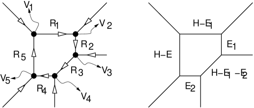
Refer to caption
Figure 12: 5-brane web dual to local B2subscript𝐵2B_{2}.

From the toric diagram we immediately obtain the SL(2,𝖹𝖹)𝑆𝐿2𝖹𝖹SL(2,{\sf Z\!\!\!Z}) matrices associated with the trivalent vertices,

(01)𝒱1(10)𝒱2(01)𝒱3(11)𝒱4(10)𝒱5(01),superscriptmaps-tosubscript𝒱1matrix01matrix10superscriptmaps-tosubscript𝒱2matrix01superscriptmaps-tosubscript𝒱3matrix11superscriptmaps-tosubscript𝒱4matrix10superscriptmaps-tosubscript𝒱5matrix01\displaystyle\pmatrix{0\cr 1}\stackrel{{\scriptstyle{\cal V}_{1}}}{{\mapsto}}\pmatrix{1\cr 0}\stackrel{{\scriptstyle{\cal V}_{2}}}{{\mapsto}}\pmatrix{0\cr-1}\stackrel{{\scriptstyle{\cal V}_{3}}}{{\mapsto}}\pmatrix{-1\cr-1}\stackrel{{\scriptstyle{\cal V}_{4}}}{{\mapsto}}\pmatrix{-1\cr 0}\stackrel{{\scriptstyle{\cal V}_{5}}}{{\mapsto}}\pmatrix{0\cr 1}\,, (59)
𝒱1=S1,𝒱2=S1,𝒱3=S1T1,𝒱4=T1S1T1,𝒱5=S1.formulae-sequencesubscript𝒱1superscript𝑆1formulae-sequencesubscript𝒱2superscript𝑆1formulae-sequencesubscript𝒱3superscript𝑆1superscript𝑇1formulae-sequencesubscript𝒱4superscript𝑇1superscript𝑆1superscript𝑇1subscript𝒱5superscript𝑆1\displaystyle{\cal V}_{1}=S^{-1}\,,\,{\cal V}_{2}=S^{-1}\,,\,{\cal V}_{3}=S^{-1}T^{-1}\,,\,{\cal V}_{4}=T^{-1}S^{-1}T^{-1}\,,\,{\cal V}_{5}=S^{-1}\,.

Using these matrices we can immediately write down the amplitude associated with the web diagram,

eFinst(c):=a=15Raeb=15lbrbi=15Ri+1|𝒱i+1|Ri,assignsuperscript𝑒subscriptsuperscript𝐹𝑐𝑖𝑛𝑠𝑡superscriptsubscript𝑎15subscriptsubscript𝑅𝑎superscript𝑒superscriptsubscript𝑏15subscript𝑙𝑏subscript𝑟𝑏superscriptsubscriptproduct𝑖15quantum-operator-productsubscript𝑅𝑖1subscript𝒱𝑖1subscript𝑅𝑖\displaystyle e^{F^{(c)}_{inst}}:=\sum_{a=1}^{5}\sum_{R_{a}}e^{-\sum_{b=1}^{5}l_{b}r_{b}}\prod_{i=1}^{5}\langle R_{i+1}|{\cal V}_{i+1}|R_{i}\rangle\,, (60)

where R6=R1subscript𝑅6subscript𝑅1R_{6}=R_{1} and 𝒱6=𝒱1subscript𝒱6subscript𝒱1{\cal V}_{6}={\cal V}_{1}. rbsubscript𝑟𝑏r_{b} are the bare Kähler parameters associated with the curve classes Cbsubscript𝐶𝑏C_{b} forming the internal line of the web,

C1=HE1,C2=E1,C3=HE1E2,C4=E2,C5=HE2.formulae-sequencesubscript𝐶1𝐻subscript𝐸1formulae-sequencesubscript𝐶2subscript𝐸1formulae-sequencesubscript𝐶3𝐻subscript𝐸1subscript𝐸2formulae-sequencesubscript𝐶4subscript𝐸2subscript𝐶5𝐻subscript𝐸2\displaystyle C_{1}=H-E_{1}\,,\,C_{2}=E_{1}\,,\,C_{3}=H-E_{1}-E_{2}\,,\,\,C_{4}=E_{2}\,,\,\,C_{5}=H-E_{2}\,. (61)

To determine the relation between rbsubscript𝑟𝑏r_{b} and the renormalized parameters associated with Cbsubscript𝐶𝑏C_{b} denoted by Tbsubscript𝑇𝑏T_{b} we calculate the terms in Eq(60) with la=δabsubscript𝑙𝑎subscript𝛿𝑎𝑏l_{a}=\delta_{ab}.

la=δabsubscript𝑙𝑎subscript𝛿𝑎𝑏l_{a}=\delta_{ab}: we denote this term by Ibsubscript𝐼𝑏I_{b},

Ibsubscript𝐼𝑏\displaystyle I_{b} =\displaystyle= (1)δb,2+δb,3+δb,4erbW 2,superscript1subscript𝛿𝑏2subscript𝛿𝑏3subscript𝛿𝑏4superscript𝑒subscript𝑟𝑏subscriptsuperscript𝑊2 \displaystyle(-1)^{\delta_{b,2}+\delta_{b,3}+\delta_{b,4}}\,e^{-r_{b}}\,W^{2}_{\vbox{\offinterlineskip\kern 1.0pt\hbox{\kern 1.0pt\vbox{\hbox{\noindent\vbox{\hbox{\vbox to0.0pt{\hrule height=0.4pt,width=3.90555pt\vss}}\hbox{\vbox{\hbox to0.0pt{\vrule width=0.4pt,height=3.90555pt\hss}}\kern 3.90555pt\vbox{\hbox to0.0pt{\vrule width=0.4pt,height=3.90555pt\hss}}}\hbox{\vbox{\hbox{\vbox to0.0pt{\hrule height=0.4pt,width=4.30554pt\vss}}}\kern-0.4pt}}}\hbox{}}\kern 1.0pt\kern 0.4pt}\kern 1.0pt\kern 0.4pt}}\,,
=\displaystyle= (1)δb,2+δb,3+δb,4erb(λ1/2λ1/2q1/2q1/2)2.superscript1subscript𝛿𝑏2subscript𝛿𝑏3subscript𝛿𝑏4superscript𝑒subscript𝑟𝑏superscriptsuperscript𝜆12superscript𝜆12superscript𝑞12superscript𝑞122\displaystyle(-1)^{\delta_{b,2}+\delta_{b,3}+\delta_{b,4}}\,e^{-r_{b}}\,(\frac{\lambda^{1/2}-\lambda^{-1/2}}{q^{1/2}-q^{-1/2}})^{2}\,.

Thus to be able to take the limit λmaps-to𝜆\lambda\mapsto\infty we define the rbsubscript𝑟𝑏r_{b} in terms of the renormalized Kähler parameters TH,TE1subscript𝑇𝐻subscript𝑇subscript𝐸1T_{H},T_{E_{1}} and TE2subscript𝑇subscript𝐸2T_{E_{2}},

r1subscript𝑟1\displaystyle r_{1} =\displaystyle= T1+log(λ)=THTE1+log(λ),subscript𝑇1log𝜆subscript𝑇𝐻subscript𝑇subscript𝐸1log𝜆\displaystyle T_{1}+\mbox{log}(\lambda)=T_{H}-T_{E_{1}}+\mbox{log}(\lambda)\,, (63)
r2subscript𝑟2\displaystyle r_{2} =\displaystyle= T2+log(λ)=TE1+log(λ),subscript𝑇2log𝜆subscript𝑇subscript𝐸1log𝜆\displaystyle T_{2}+\mbox{log}(\lambda)=T_{E_{1}}+\mbox{log}(\lambda)\,,
r3subscript𝑟3\displaystyle r_{3} =\displaystyle= T3+log(λ)=THTE1TE2+log(λ),subscript𝑇3log𝜆subscript𝑇𝐻subscript𝑇subscript𝐸1subscript𝑇subscript𝐸2log𝜆\displaystyle T_{3}+\mbox{log}(\lambda)=T_{H}-T_{E_{1}}-T_{E_{2}}+\mbox{log}(\lambda)\,,
r4subscript𝑟4\displaystyle r_{4} =\displaystyle= T4+log(λ)=TE2+log(λ),subscript𝑇4log𝜆subscript𝑇subscript𝐸2log𝜆\displaystyle T_{4}+\mbox{log}(\lambda)=T_{E_{2}}+\mbox{log}(\lambda)\,,
r5subscript𝑟5\displaystyle r_{5} =\displaystyle= T5+log(λ)=THTE2+log(λ)subscript𝑇5log𝜆subscript𝑇𝐻subscript𝑇subscript𝐸2log𝜆\displaystyle T_{5}+\mbox{log}(\lambda)=T_{H}-T_{E_{2}}+\mbox{log}(\lambda)\,

5.3.1 Integer invariants of few curve classes

Using the above definition of TH,E1,E2subscript𝑇𝐻subscript𝐸1subscript𝐸2T_{H,E_{1},E_{2}} we can write the amplitude Eq(60) as

eFinst(c)=a=15Rae(lHTHlE1TE1lE2TE2)(1)l2+l3+l4q12(κR2+κR3+κR4)i=15𝒲Ri+1,Ri.superscript𝑒subscriptsuperscript𝐹𝑐𝑖𝑛𝑠𝑡superscriptsubscript𝑎15subscriptsubscript𝑅𝑎superscript𝑒subscript𝑙𝐻subscript𝑇𝐻subscript𝑙subscript𝐸1subscript𝑇subscript𝐸1subscript𝑙subscript𝐸2subscript𝑇subscript𝐸2superscript1subscript𝑙2subscript𝑙3subscript𝑙4superscript𝑞12subscript𝜅subscript𝑅2subscript𝜅subscript𝑅3subscript𝜅subscript𝑅4superscriptsubscriptproduct𝑖15subscript𝒲subscript𝑅𝑖1subscript𝑅𝑖\displaystyle e^{F^{(c)}_{inst}}=\sum_{a=1}^{5}\sum_{R_{a}}e^{-(l_{H}T_{H}-l_{E_{1}}T_{E_{1}}-l_{E_{2}}T_{E_{2}})}\,\,(-1)^{l_{2}+l_{3}+l_{4}}\,q^{-\frac{1}{2}(\kappa_{R_{2}}+\kappa_{R_{3}}+\kappa_{R_{4}})}\,\,\prod_{i=1}^{5}{\cal W}_{R_{i+1},R_{i}}\,. (64)

where

lH=l1+l3+l5,lE1=l1+l3l2,lE2=l3+l5l4.formulae-sequencesubscript𝑙𝐻subscript𝑙1subscript𝑙3subscript𝑙5formulae-sequencesubscript𝑙subscript𝐸1subscript𝑙1subscript𝑙3subscript𝑙2subscript𝑙subscript𝐸2subscript𝑙3subscript𝑙5subscript𝑙4\displaystyle l_{H}=l_{1}+l_{3}+l_{5}\,,\,\,l_{E_{1}}=l_{1}+l_{3}-l_{2}\,,\,\,l_{E_{2}}=l_{3}+l_{5}-l_{4}\,. (65)

we start with determining the invariants associated with the exceptional curves E1,E2subscript𝐸1subscript𝐸2E_{1},E_{2} and HE1E2𝐻subscript𝐸1subscript𝐸2H-E_{1}-E_{2}.

E1subscript𝐸1E_{1}:  This term, which we will denote by (E1)subscript𝐸1{\cal I}(E_{1}), is given by (l1,l2,l3,l4,l5)=(0,1,0,0,0)subscript𝑙1subscript𝑙2subscript𝑙3subscript𝑙4subscript𝑙501000(l_{1},l_{2},l_{3},l_{4},l_{5})=(0,1,0,0,0),

(E1)subscript𝐸1\displaystyle{\cal I}(E_{1}) =\displaystyle= eTE1𝒲 2,superscript𝑒subscript𝑇subscript𝐸1subscriptsuperscript𝒲2 \displaystyle-e^{-T_{E_{1}}}\,{\cal W}^{2}_{\vbox{\offinterlineskip\kern 1.0pt\hbox{\kern 1.0pt\vbox{\hbox{\noindent\vbox{\hbox{\vbox to0.0pt{\hrule height=0.4pt,width=3.90555pt\vss}}\hbox{\vbox{\hbox to0.0pt{\vrule width=0.4pt,height=3.90555pt\hss}}\kern 3.90555pt\vbox{\hbox to0.0pt{\vrule width=0.4pt,height=3.90555pt\hss}}}\hbox{\vbox{\hbox{\vbox to0.0pt{\hrule height=0.4pt,width=4.30554pt\vss}}}\kern-0.4pt}}}\hbox{}}\kern 1.0pt\kern 0.4pt}\kern 1.0pt\kern 0.4pt}}\,,
=\displaystyle= eTE1(2sin(gs/2))2.superscript𝑒subscript𝑇subscript𝐸1superscript2sinsubscript𝑔𝑠22\displaystyle\frac{e^{-T_{E_{1}}}}{(2\mbox{sin}(g_{s}/2))^{2}}\,.

This implies that

NE10=1,NE1g=0,g>0.formulae-sequencesubscriptsuperscript𝑁0subscript𝐸11formulae-sequencesubscriptsuperscript𝑁𝑔subscript𝐸10𝑔0\displaystyle N^{0}_{E_{1}}=1\,,\,\,\,N^{g}_{E_{1}}=0\,,\,g>0\,. (67)

Similarly the term corresponding to E2subscript𝐸2E_{2} is the same as above giving NE20=1subscriptsuperscript𝑁0subscript𝐸21N^{0}_{E_{2}}=1 and NE2gsubscriptsuperscript𝑁𝑔subscript𝐸2N^{g}_{E_{2}} for g>0𝑔0g>0 as expected since the exceptional curves are rigid with zero dimensional moduli space.

HE1E2𝐻subscript𝐸1subscript𝐸2H-E_{1}-E_{2}  There is only term which contributes here given by (l1,l2,l3,l4,l5)=(0,0,1,0,0)subscript𝑙1subscript𝑙2subscript𝑙3subscript𝑙4subscript𝑙500100(l_{1},l_{2},l_{3},l_{4},l_{5})=(0,0,1,0,0),

(HE1E2)𝐻subscript𝐸1subscript𝐸2\displaystyle{\cal I}(H-E_{1}-E_{2}) =\displaystyle= e(THTE1TE2)𝒲 2,superscript𝑒subscript𝑇𝐻subscript𝑇subscript𝐸1subscript𝑇subscript𝐸2subscriptsuperscript𝒲2 \displaystyle-e^{-(T_{H}-T_{E_{1}}-T_{E_{2}})}\,{\cal W}^{2}_{\vbox{\offinterlineskip\kern 1.0pt\hbox{\kern 1.0pt\vbox{\hbox{\noindent\vbox{\hbox{\vbox to0.0pt{\hrule height=0.4pt,width=3.90555pt\vss}}\hbox{\vbox{\hbox to0.0pt{\vrule width=0.4pt,height=3.90555pt\hss}}\kern 3.90555pt\vbox{\hbox to0.0pt{\vrule width=0.4pt,height=3.90555pt\hss}}}\hbox{\vbox{\hbox{\vbox to0.0pt{\hrule height=0.4pt,width=4.30554pt\vss}}}\kern-0.4pt}}}\hbox{}}\kern 1.0pt\kern 0.4pt}\kern 1.0pt\kern 0.4pt}}\,,
=\displaystyle= eTH+TE1+TE2(2sin(gs/2))2.superscript𝑒subscript𝑇𝐻subscript𝑇subscript𝐸1subscript𝑇subscript𝐸2superscript2sinsubscript𝑔𝑠22\displaystyle\frac{e^{-T_{H}+T_{E_{1}}+T_{E_{2}}}}{(2\mbox{sin}(g_{s}/2))^{2}}\,.

Thus we get NHE1E2g=δg,0subscriptsuperscript𝑁𝑔𝐻subscript𝐸1subscript𝐸2subscript𝛿𝑔0N^{g}_{H-E_{1}-E_{2}}=\delta_{g,0} since HE1E2𝐻subscript𝐸1subscript𝐸2H-E_{1}-E_{2} is an exceptional curve.

5.4 3subscript3{\cal B}_{3}

The web diagram in this case is given by Fig. 13.
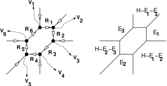
Refer to caption
Figure 13: 5-brane web dual to local 3subscript3{\cal B}_{3}.

The SL(2,𝖹𝖹)𝑆𝐿2𝖹𝖹SL(2,{\sf Z\!\!\!Z}) matrices are determined by the web diagram and are

(11)𝒱1(10)𝒱2(01)𝒱3(11)𝒱4(10)𝒱5(01)𝒱6(11),superscriptmaps-tosubscript𝒱1matrix11matrix10superscriptmaps-tosubscript𝒱2matrix01superscriptmaps-tosubscript𝒱3matrix11superscriptmaps-tosubscript𝒱4matrix10superscriptmaps-tosubscript𝒱5matrix01superscriptmaps-tosubscript𝒱6matrix11\displaystyle\pmatrix{1\cr 1}\stackrel{{\scriptstyle{\cal V}_{1}}}{{\mapsto}}\pmatrix{1\cr 0}\stackrel{{\scriptstyle{\cal V}_{2}}}{{\mapsto}}\pmatrix{0\cr-1}\stackrel{{\scriptstyle{\cal V}_{3}}}{{\mapsto}}\pmatrix{-1\cr-1}\stackrel{{\scriptstyle{\cal V}_{4}}}{{\mapsto}}\pmatrix{-1\cr 0}\stackrel{{\scriptstyle{\cal V}_{5}}}{{\mapsto}}\pmatrix{0\cr 1}\stackrel{{\scriptstyle{\cal V}_{6}}}{{\mapsto}}\pmatrix{1\cr 1}\,, (69)
𝒱1=T1S1T1,𝒱2=S1,𝒱3=S1T1,𝒱4=T1S1T1,𝒱5=S1,𝒱6=S1T1.formulae-sequencesubscript𝒱1superscript𝑇1superscript𝑆1superscript𝑇1formulae-sequencesubscript𝒱2superscript𝑆1formulae-sequencesubscript𝒱3superscript𝑆1superscript𝑇1formulae-sequencesubscript𝒱4superscript𝑇1superscript𝑆1superscript𝑇1formulae-sequencesubscript𝒱5superscript𝑆1subscript𝒱6superscript𝑆1superscript𝑇1\displaystyle{\cal V}_{1}=T^{-1}S^{-1}T^{-1}\,,\,{\cal V}_{2}=S^{-1}\,,\,{\cal V}_{3}=S^{-1}T^{-1}\,,\,{\cal V}_{4}=T^{-1}S^{-1}T^{-1}\,,\,{\cal V}_{5}=S^{-1}\,,\,{\cal V}_{6}=S^{-1}T^{-1}\,.

Then Finst(c)subscriptsuperscript𝐹𝑐𝑖𝑛𝑠𝑡F^{(c)}_{inst} is given by

eFinst(c)=a=16Raeb=16lbrbb=16Rb+1|𝒱b+1|Rb.superscript𝑒subscriptsuperscript𝐹𝑐𝑖𝑛𝑠𝑡superscriptsubscript𝑎16subscriptsubscript𝑅𝑎superscript𝑒superscriptsubscript𝑏16subscript𝑙𝑏subscript𝑟𝑏superscriptsubscriptproduct𝑏16quantum-operator-productsubscript𝑅𝑏1subscript𝒱𝑏1subscript𝑅𝑏\displaystyle e^{F^{(c)}_{inst}}=\sum_{a=1}^{6}\sum_{R_{a}}e^{-\sum_{b=1}^{6}l_{b}r_{b}}\prod_{b=1}^{6}\langle R_{b+1}|{\cal V}_{b+1}|R_{b}\rangle\,. (70)

Where R7=R1subscript𝑅7subscript𝑅1R_{7}=R_{1} and 𝒱7=𝒱1subscript𝒱7subscript𝒱1{\cal V}_{7}={\cal V}_{1}. calculation similar to the one done before gives the rbsubscript𝑟𝑏r_{b} in terms of normalized Kähler parameters TH,TE1,TE2,TE3subscript𝑇𝐻subscript𝑇subscript𝐸1subscript𝑇subscript𝐸2subscript𝑇subscript𝐸3T_{H},T_{E_{1}},T_{E_{2}},T_{E_{3}},

r1subscript𝑟1\displaystyle r_{1} =\displaystyle= THTE1TE3+log(λ),subscript𝑇𝐻subscript𝑇subscript𝐸1subscript𝑇subscript𝐸3log𝜆\displaystyle T_{H}-T_{E_{1}}-T_{E_{3}}+\mbox{log}(\lambda)\,, (71)
r2subscript𝑟2\displaystyle r_{2} =\displaystyle= TE1+log(λ),subscript𝑇subscript𝐸1log𝜆\displaystyle T_{E_{1}}+\mbox{log}(\lambda)\,,
r3subscript𝑟3\displaystyle r_{3} =\displaystyle= THTE1TE2+log(λ),subscript𝑇𝐻subscript𝑇subscript𝐸1subscript𝑇subscript𝐸2log𝜆\displaystyle T_{H}-T_{E_{1}}-T_{E_{2}}+\mbox{log}(\lambda)\,,
r4subscript𝑟4\displaystyle r_{4} =\displaystyle= TE2+log(λ),subscript𝑇subscript𝐸2log𝜆\displaystyle T_{E_{2}}+\mbox{log}(\lambda)\,,
r5subscript𝑟5\displaystyle r_{5} =\displaystyle= THTE2TE3+log(λ),subscript𝑇𝐻subscript𝑇subscript𝐸2subscript𝑇subscript𝐸3log𝜆\displaystyle T_{H}-T_{E_{2}}-T_{E_{3}}+\mbox{log}(\lambda)\,,
r6subscript𝑟6\displaystyle r_{6} =\displaystyle= TE3+log(λ).subscript𝑇subscript𝐸3log𝜆\displaystyle T_{E_{3}}+\mbox{log}(\lambda)\,.

5.4.1 Integer invariants of few curve classes

To show that this correctly reproduces the integer invariants [10] we calculate some terms in the above expansion corresponding to exceptional curves. First we rewrite Eq(70) in terms of TH,TE1,TE2,TE3subscript𝑇𝐻subscript𝑇subscript𝐸1subscript𝑇subscript𝐸2subscript𝑇subscript𝐸3T_{H},T_{E_{1}},T_{E_{2}},T_{E_{3}},

eFinst(c)=a=16Rae(lHTHlE1TE1lE2TE2)(1)i=16liq12(i=16κRi)b=16𝒲Rb+1,Rbsuperscript𝑒subscriptsuperscript𝐹𝑐𝑖𝑛𝑠𝑡superscriptsubscript𝑎16subscriptsubscript𝑅𝑎superscript𝑒subscript𝑙𝐻subscript𝑇𝐻subscript𝑙subscript𝐸1subscript𝑇subscript𝐸1subscript𝑙subscript𝐸2subscript𝑇subscript𝐸2superscript1superscriptsubscript𝑖16subscript𝑙𝑖superscript𝑞12superscriptsubscript𝑖16subscript𝜅subscript𝑅𝑖superscriptsubscriptproduct𝑏16subscript𝒲subscript𝑅𝑏1subscript𝑅𝑏\displaystyle e^{F^{(c)}_{inst}}=\sum_{a=1}^{6}\sum_{R_{a}}e^{-(l_{H}T_{H}-l_{E_{1}}T_{E_{1}}-l_{E_{2}}T_{E_{2}})}\,(-1)^{\sum_{i=1}^{6}l_{i}}q^{-\frac{1}{2}(\sum_{i=1}^{6}\kappa_{R_{i}})}\,\prod_{b=1}^{6}{\cal W}_{R_{b+1},R_{b}} (72)

Where

lH=l1+l3+l5,lE1=l1+l3l2,lE2=l3+l5l4,lE3=l1+l5l6.formulae-sequencesubscript𝑙𝐻subscript𝑙1subscript𝑙3subscript𝑙5formulae-sequencesubscript𝑙subscript𝐸1subscript𝑙1subscript𝑙3subscript𝑙2formulae-sequencesubscript𝑙subscript𝐸2subscript𝑙3subscript𝑙5subscript𝑙4subscript𝑙subscript𝐸3subscript𝑙1subscript𝑙5subscript𝑙6\displaystyle l_{H}=l_{1}+l_{3}+l_{5}\,,\,\,l_{E_{1}}=l_{1}+l_{3}-l_{2}\,,\,\,l_{E_{2}}=l_{3}+l_{5}-l_{4}\,,\,\,l_{E_{3}}=l_{1}+l_{5}-l_{6}\,. (73)

Easubscript𝐸𝑎E_{a}: In this case we have to take l1=l3=l5=0subscript𝑙1subscript𝑙3subscript𝑙50l_{1}=l_{3}=l_{5}=0 and la=δa,2+δa,4=δa,6subscript𝑙𝑎subscript𝛿𝑎2subscript𝛿𝑎4subscript𝛿𝑎6l_{a}=\delta_{a,2}+\delta_{a,4}=\delta_{a,6}.

(Ea)subscript𝐸𝑎\displaystyle{\cal I}(E_{a}) =\displaystyle= eTEa,𝒲 2,superscript𝑒subscript𝑇subscript𝐸𝑎subscriptsuperscript𝒲2 \displaystyle-e^{-T_{E_{a}}},{\cal W}^{2}_{\vbox{\offinterlineskip\kern 1.0pt\hbox{\kern 1.0pt\vbox{\hbox{\noindent\vbox{\hbox{\vbox to0.0pt{\hrule height=0.4pt,width=3.90555pt\vss}}\hbox{\vbox{\hbox to0.0pt{\vrule width=0.4pt,height=3.90555pt\hss}}\kern 3.90555pt\vbox{\hbox to0.0pt{\vrule width=0.4pt,height=3.90555pt\hss}}}\hbox{\vbox{\hbox{\vbox to0.0pt{\hrule height=0.4pt,width=4.30554pt\vss}}}\kern-0.4pt}}}\hbox{}}\kern 1.0pt\kern 0.4pt}\kern 1.0pt\kern 0.4pt}}\,,
=\displaystyle= eTEa(2sin(gs/2))2.superscript𝑒subscript𝑇subscript𝐸𝑎superscript2sinsubscript𝑔𝑠22\displaystyle\frac{e^{-T_{E_{a}}}}{(2\mbox{sin}(g_{s}/2))^{2}}\,.

Thus we get as expected NEag=δg,0subscriptsuperscript𝑁𝑔subscript𝐸𝑎subscript𝛿𝑔0N^{g}_{E_{a}}=\delta_{g,0}.

HEaEb,ab𝐻subscript𝐸𝑎subscript𝐸𝑏𝑎𝑏H-E_{a}-E_{b},a\neq b: In this case we have only one term contributing for each curve. For HE1E3𝐻subscript𝐸1subscript𝐸3H-E_{1}-E_{3} we have la=(0,0,1,0,0,0)subscript𝑙𝑎001000l_{a}=(0,0,1,0,0,0), for HE1E3𝐻subscript𝐸1subscript𝐸3H-E_{1}-E_{3} we have la=(0,1,0,0,0,0)subscript𝑙𝑎010000l_{a}=(0,1,0,0,0,0) and for HE2E3𝐻subscript𝐸2subscript𝐸3H-E_{2}-E_{3} we have la=(1,0,0,0,0,0)subscript𝑙𝑎100000l_{a}=(1,0,0,0,0,0). Thus we get

(HEaEb)𝐻subscript𝐸𝑎subscript𝐸𝑏\displaystyle{\cal I}(H-E_{a}-E_{b}) =\displaystyle= e(THTEaTEb)𝒲 2,superscript𝑒subscript𝑇𝐻subscript𝑇subscript𝐸𝑎subscript𝑇subscript𝐸𝑏subscriptsuperscript𝒲2 \displaystyle-e^{-(T_{H}-T_{E_{a}}-T_{E_{b}})}\,{\cal W}^{2}_{\vbox{\offinterlineskip\kern 1.0pt\hbox{\kern 1.0pt\vbox{\hbox{\noindent\vbox{\hbox{\vbox to0.0pt{\hrule height=0.4pt,width=3.90555pt\vss}}\hbox{\vbox{\hbox to0.0pt{\vrule width=0.4pt,height=3.90555pt\hss}}\kern 3.90555pt\vbox{\hbox to0.0pt{\vrule width=0.4pt,height=3.90555pt\hss}}}\hbox{\vbox{\hbox{\vbox to0.0pt{\hrule height=0.4pt,width=4.30554pt\vss}}}\kern-0.4pt}}}\hbox{}}\kern 1.0pt\kern 0.4pt}\kern 1.0pt\kern 0.4pt}}\,,
=\displaystyle= e(THTE1TE2)(2sin(gs/2))2.superscript𝑒subscript𝑇𝐻subscript𝑇subscript𝐸1subscript𝑇subscript𝐸2superscript2sinsubscript𝑔𝑠22\displaystyle\frac{e^{-(T_{H}-T_{E_{1}}-T_{E_{2}})}}{(2\mbox{sin}(g_{s}/2))^{2}}\,.

Thus again we get the correct result NHEaEbg=δg,0subscriptsuperscript𝑁𝑔𝐻subscript𝐸𝑎subscript𝐸𝑏subscript𝛿𝑔0N^{g}_{H-E_{a}-E_{b}}=\delta_{g,0}.

5.5 F0=IP1×IP1subscript𝐹0IsuperscriptP1IsuperscriptP1F_{0}=\mbox{I}\!\mbox{P}^{1}\times\mbox{I}\!\mbox{P}^{1}

This case was discussed in detail in [21]. We include this here for completeness. The web diagram is shown in Fig. 14 from which we get the following SL(2,𝖹𝖹)𝑆𝐿2𝖹𝖹SL(2,{\sf Z\!\!\!Z}) matrices associated with the vertices.

Refer to caption
Figure 14: 5-brane web dual to local IP1×IP1IsuperscriptP1IsuperscriptP1\mbox{I}\!\mbox{P}^{1}\times\mbox{I}\!\mbox{P}^{1}.
(10)𝒱1(01)𝒱2(10)𝒱3(01)𝒱4(10),superscriptmaps-tosubscript𝒱1matrix10matrix01superscriptmaps-tosubscript𝒱2matrix10superscriptmaps-tosubscript𝒱3matrix01superscriptmaps-tosubscript𝒱4matrix10\displaystyle\pmatrix{1\cr 0}\stackrel{{\scriptstyle{\cal V}_{1}}}{{\mapsto}}\pmatrix{0\cr-1}\stackrel{{\scriptstyle{\cal V}_{2}}}{{\mapsto}}\pmatrix{-1\cr 0}\stackrel{{\scriptstyle{\cal V}_{3}}}{{\mapsto}}\pmatrix{0\cr 1}\stackrel{{\scriptstyle{\cal V}_{4}}}{{\mapsto}}\pmatrix{1\cr 0}\,, (76)
𝒱1=𝒱2=𝒱3=𝒱4=S1.subscript𝒱1subscript𝒱2subscript𝒱3subscript𝒱4superscript𝑆1\displaystyle{\cal V}_{1}={\cal V}_{2}={\cal V}_{3}={\cal V}_{4}=S^{-1}\,.

The amplitude associated with it is then given by

eFinst(c)=a=14Raea=14larab=14Rb+1|𝒱b+1|Rb.superscript𝑒subscriptsuperscript𝐹𝑐𝑖𝑛𝑠𝑡superscriptsubscript𝑎14subscriptsubscript𝑅𝑎superscript𝑒superscriptsubscript𝑎14subscript𝑙𝑎subscript𝑟𝑎superscriptsubscriptproduct𝑏14quantum-operator-productsubscript𝑅𝑏1subscript𝒱𝑏1subscript𝑅𝑏\displaystyle e^{F^{(c)}_{inst}}=\sum_{a=1}^{4}\sum_{R_{a}}e^{-\sum_{a=1}^{4}l_{a}r_{a}}\,\prod_{b=1}^{4}\langle R_{b+1}|{\cal V}_{b+1}|R_{b}\rangle. (77)

Where we have R5=R1subscript𝑅5subscript𝑅1R_{5}=R_{1} and 𝒱5=𝒱1subscript𝒱5subscript𝒱1{\cal V}_{5}={\cal V}_{1}. This is exactly the expression obtained in [21] using geometric transition of F0subscript𝐹0F_{0} blown up at four points. The relation between the renormalized Kähler parameters and r1,2subscript𝑟12r_{1,2} can be obtained from the terms with only one lasubscript𝑙𝑎l_{a} non-vanishing.

la=δabsubscript𝑙𝑎subscript𝛿𝑎𝑏l_{a}=\delta_{ab}

Ibsubscript𝐼𝑏\displaystyle I_{b} =\displaystyle= erbW 2,superscript𝑒subscript𝑟𝑏subscriptsuperscript𝑊2 \displaystyle e^{-r_{b}}W^{2}_{\vbox{\offinterlineskip\kern 1.0pt\hbox{\kern 1.0pt\vbox{\hbox{\noindent\vbox{\hbox{\vbox to0.0pt{\hrule height=0.4pt,width=3.90555pt\vss}}\hbox{\vbox{\hbox to0.0pt{\vrule width=0.4pt,height=3.90555pt\hss}}\kern 3.90555pt\vbox{\hbox to0.0pt{\vrule width=0.4pt,height=3.90555pt\hss}}}\hbox{\vbox{\hbox{\vbox to0.0pt{\hrule height=0.4pt,width=4.30554pt\vss}}}\kern-0.4pt}}}\hbox{}}\kern 1.0pt\kern 0.4pt}\kern 1.0pt\kern 0.4pt}}\,,
=\displaystyle= erb(λ1/2λ1/2q1/2q1/2)2.superscript𝑒subscript𝑟𝑏superscriptsuperscript𝜆12superscript𝜆12superscript𝑞12superscript𝑞122\displaystyle e^{-r_{b}}\,(\frac{\lambda^{1/2}-\lambda^{-1/2}}{q^{1/2}-q^{-1/2}})^{2}\,.

Thus λmaps-to𝜆\lambda\mapsto\infty limit implies that we have to define the renormalized Tl1subscript𝑇subscript𝑙1T_{l_{1}} and Tl2subscript𝑇subscript𝑙2T_{l_{2}} as follows

r1=r3=Tl1+log(λ),subscript𝑟1subscript𝑟3subscript𝑇subscript𝑙1log𝜆\displaystyle r_{1}=r_{3}=T_{l_{1}}+\mbox{log}(\lambda)\,, (79)
r2=r4=Tl2+log(λ).subscript𝑟2subscript𝑟4subscript𝑇subscript𝑙2log𝜆\displaystyle r_{2}=r_{4}=T_{l_{2}}+\mbox{log}(\lambda)\,.

Here l1,2subscript𝑙12l_{1,2} are the two IP1IsuperscriptP1\mbox{I}\!\mbox{P}^{1} such that

lalb=1δab.subscript𝑙𝑎subscript𝑙𝑏1subscript𝛿𝑎𝑏\displaystyle l_{a}\cdot l_{b}=1-\delta_{ab}\,. (80)

5.6 F2subscript𝐹2F_{2}

Now consider the case of local CY manifold which has compact divisor F2subscript𝐹2F_{2}, the second Hirzebruch surface. We consider this cases since it would be difficult to analyze using the geometric transition technique [21, 20]. The toric diagrams are shown in Fig. 8 form which we can obtain the the web diagram as shown in Fig. 15. In this case also to begin with we have to determine which curve classes Casubscript𝐶𝑎C_{a} correspond to the four internal lines of the web diagram.

Refer to caption
Figure 15: 5-brane web dual to local F2subscript𝐹2F_{2}.

Homology, Kähler parameters, gluing matrices and the Riemann surface: Second Hirzebruch surface F2subscript𝐹2F_{2} like F0subscript𝐹0F_{0} and B1=F1subscript𝐵1subscript𝐹1B_{1}=F_{1} is a IP1IsuperscriptP1\mbox{I}\!\mbox{P}^{1} bundle over IP1IsuperscriptP1\mbox{I}\!\mbox{P}^{1} and has a two dimensional second homology group spanned by the class of the base IP1IsuperscriptP1\mbox{I}\!\mbox{P}^{1} and the class of the fiber IP1IsuperscriptP1\mbox{I}\!\mbox{P}^{1} which we denote with B𝐵B and F𝐹F respectively. The class dual to the first Chern class is given by 2B+4F2𝐵4𝐹2B+4F and the intersection numbers are given by

BB=2,BF=1,FF=0.formulae-sequence𝐵𝐵2formulae-sequence𝐵𝐹1𝐹𝐹0\displaystyle B\cdot B=-2\,,\,\,\,B\cdot F=1\,,\,\,\,F\cdot F=0\,. (81)

From the web diagram it is clear that the curve between the two vertices with parallel external legs is a curve of self-intersection -2 and therefore C3=Bsubscript𝐶3𝐵C_{3}=B. Also it is clear that C2=C4=Fsubscript𝐶2subscript𝐶4𝐹C_{2}=C_{4}=F since F𝐹F is the only rational curve which intersects B𝐵B at one point. Since a=14Ca=2B+4Fsuperscriptsubscript𝑎14subscript𝐶𝑎2𝐵4𝐹\sum_{a=1}^{4}C_{a}=2B+4F (class dual to the first Chern class) thus C1=B+2Fsubscript𝐶1𝐵2𝐹C_{1}=B+2F.

Form Fig. 15 we can easily determine the gluing matrices as the SL(2,𝖹𝖹)𝑆𝐿2𝖹𝖹SL(2,{\sf Z\!\!\!Z}) matrix associated with a vertex which maps an incoming internal line into the outgoing internal line at that vertex. With the orientation of the lines as shown in Fig. 15 we get

𝒱1=TS1,𝒱2=S1T1,𝒱3=T1S1,𝒱4=S1T.formulae-sequencesubscript𝒱1𝑇superscript𝑆1formulae-sequencesubscript𝒱2superscript𝑆1superscript𝑇1formulae-sequencesubscript𝒱3superscript𝑇1superscript𝑆1subscript𝒱4superscript𝑆1𝑇\displaystyle{\cal V}_{1}=TS^{-1}\,,\,\,{\cal V}_{2}=S^{-1}T^{-1}\,,\,\,\,{\cal V}_{3}=T^{-1}S^{-1}\,,\,\,\,{\cal V}_{4}=S^{-1}T\,. (82)

The web diagram also completely determines the equation of the Riemann surface obtained by thickening the web. As discussed before the theory on the M5-brane wrapped on this Riemann surface is dual to the N=2𝑁2N=2 theory obtained by compactifying Type IIA string theory on the local F2subscript𝐹2F_{2}. The equation for the Riemann surface for the local F2subscript𝐹2F_{2} case is given by

1+eu+ev+et1u+et22uv=0.1superscript𝑒𝑢superscript𝑒𝑣superscript𝑒subscript𝑡1𝑢superscript𝑒subscript𝑡22𝑢𝑣0\displaystyle 1+e^{u}+e^{v}+e^{-t_{1}-u}+e^{-t_{2}-2u-v}=0\,. (83)

Where t1,2subscript𝑡12t_{1,2} are Kähler parameters and u,vCI𝑢𝑣CIu,v\in\mbox{C}\!\!\!\mbox{I}.

Topological string amplitude and renormalized Kähler parameter: Using the above gluing matrices one can immediately write down the closed string topological amplitude by interpreting the Riemann surface associated with the above web diagram as a Feynman digram with operators 𝒱asubscript𝒱𝑎{\cal V}_{a} giving the interactions at the vertices.

eF(c)superscript𝑒subscript𝐹𝑐\displaystyle e^{F_{(c)}} =\displaystyle= Raea=14laraR1|𝒱4|R4,0R4|𝒱3|R3,0R3|𝒱2|R2,0R2|𝒱1|R1,0,subscriptsubscript𝑅𝑎superscript𝑒superscriptsubscript𝑎14subscript𝑙𝑎subscript𝑟𝑎quantum-operator-productsubscript𝑅1subscript𝒱4subscript𝑅40quantum-operator-productsubscript𝑅4subscript𝒱3subscript𝑅30quantum-operator-productsubscript𝑅3subscript𝒱2subscript𝑅20quantum-operator-productsubscript𝑅2subscript𝒱1subscript𝑅10\displaystyle\sum_{R_{a}}e^{-\sum_{a=1}^{4}l_{a}r_{a}}\,\langle R_{1}|{\cal V}_{4}|R_{4},0\rangle\langle R_{4}|{\cal V}_{3}|R_{3},0\rangle\,\langle R_{3}|{\cal V}_{2}|R_{2},0\rangle\langle R_{2}|{\cal V}_{1}|R_{1},0\rangle\,,
=\displaystyle= Raea=14laraR1|S1T|R4R4|T1S1|R3R3|S1T1|R2R2|TS1|R1.subscriptsubscript𝑅𝑎superscript𝑒superscriptsubscript𝑎14subscript𝑙𝑎subscript𝑟𝑎quantum-operator-productsubscript𝑅1superscript𝑆1𝑇subscript𝑅4quantum-operator-productsubscript𝑅4superscript𝑇1superscript𝑆1subscript𝑅3quantum-operator-productsubscript𝑅3superscript𝑆1superscript𝑇1subscript𝑅2quantum-operator-productsubscript𝑅2𝑇superscript𝑆1subscript𝑅1\displaystyle\sum_{R_{a}}e^{-\sum_{a=1}^{4}l_{a}r_{a}}\,\langle R_{1}|S^{-1}T|R_{4}\rangle\langle R_{4}|T^{-1}S^{-1}|R_{3}\rangle\,\langle R_{3}|S^{-1}T^{-1}|R_{2}\rangle\langle R_{2}|TS^{-1}|R_{1}\rangle\,.

To determine the renormalized Kähler parameters TB,TFsubscript𝑇𝐵subscript𝑇𝐹T_{B},T_{F} in terms of rasubscript𝑟𝑎r_{a} we determine terms with only one lasubscript𝑙𝑎l_{a} non-vanishing.

la=δabsubscript𝑙𝑎subscript𝛿𝑎𝑏l_{a}=\delta_{ab}: we denote this term by bsubscript𝑏{\cal I}_{b} and it is the coefficient of erbsuperscript𝑒subscript𝑟𝑏e^{-r_{b}} in Eq(5.6),

bsubscript𝑏\displaystyle{\cal I}_{b} =\displaystyle= erb |S1|00|S1| ,superscript𝑒subscript𝑟𝑏quantum-operator-product superscript𝑆10quantum-operator-product0superscript𝑆1 \displaystyle e^{-r_{b}}\,\langle\vbox{\offinterlineskip\kern 1.0pt\hbox{\kern 1.0pt\vbox{\hbox{\noindent\vbox{\hbox{\vbox to0.0pt{\hrule height=0.4pt,width=3.90555pt\vss}}\hbox{\vbox{\hbox to0.0pt{\vrule width=0.4pt,height=3.90555pt\hss}}\kern 3.90555pt\vbox{\hbox to0.0pt{\vrule width=0.4pt,height=3.90555pt\hss}}}\hbox{\vbox{\hbox{\vbox to0.0pt{\hrule height=0.4pt,width=4.30554pt\vss}}}\kern-0.4pt}}}\hbox{}}\kern 1.0pt\kern 0.4pt}\kern 1.0pt\kern 0.4pt}|S^{-1}|0\rangle\,\langle 0|S^{-1}|\vbox{\offinterlineskip\kern 1.0pt\hbox{\kern 1.0pt\vbox{\hbox{\noindent\vbox{\hbox{\vbox to0.0pt{\hrule height=0.4pt,width=3.90555pt\vss}}\hbox{\vbox{\hbox to0.0pt{\vrule width=0.4pt,height=3.90555pt\hss}}\kern 3.90555pt\vbox{\hbox to0.0pt{\vrule width=0.4pt,height=3.90555pt\hss}}}\hbox{\vbox{\hbox{\vbox to0.0pt{\hrule height=0.4pt,width=4.30554pt\vss}}}\kern-0.4pt}}}\hbox{}}\kern 1.0pt\kern 0.4pt}\kern 1.0pt\kern 0.4pt}\rangle\,,
=\displaystyle= erb(λ1/2λ1/22sin(gs/2))2,superscript𝑒subscript𝑟𝑏superscriptsuperscript𝜆12superscript𝜆122sinsubscript𝑔𝑠22\displaystyle-e^{-r_{b}}(\frac{\lambda^{1/2}-\lambda^{-1/2}}{2\mbox{sin}(g_{s}/2)})^{2}\,,
=\displaystyle= eTb(2sin(gs/2))2.superscript𝑒subscript𝑇𝑏superscript2sinsubscript𝑔𝑠22\displaystyle-\frac{e^{-T_{b}}}{(2\mbox{sin}(g_{s}/2))^{2}}\,.

Where in the last line we have taken the limit λmaps-to𝜆\lambda\mapsto\infty after defining the renormalized Kähler parameter TCbsubscript𝑇subscript𝐶𝑏T_{C_{b}} associated with the curve Cbsubscript𝐶𝑏C_{b} such that

rb=TCb+log(λ).subscript𝑟𝑏subscript𝑇subscript𝐶𝑏log𝜆\displaystyle r_{b}=T_{C_{b}}+\mbox{log}(\lambda)\,. (86)

Thus we get the following relations between rasubscript𝑟𝑎r_{a} and TCasubscript𝑇subscript𝐶𝑎T_{C_{a}},

r1subscript𝑟1\displaystyle r_{1} =\displaystyle= TB+2F+log(λ)=TB+2TF+log(λ)subscript𝑇𝐵2𝐹log𝜆subscript𝑇𝐵2subscript𝑇𝐹log𝜆\displaystyle T_{B+2F}+\mbox{log}(\lambda)=T_{B}+2T_{F}+\mbox{log}(\lambda)\, (87)
r2subscript𝑟2\displaystyle r_{2} =\displaystyle= TF+log(λ),subscript𝑇𝐹log𝜆\displaystyle T_{F}+\mbox{log}(\lambda)\,,
r3subscript𝑟3\displaystyle r_{3} =\displaystyle= TB+log(λ),subscript𝑇𝐵log𝜆\displaystyle T_{B}+\mbox{log}(\lambda)\,,
r4subscript𝑟4\displaystyle r_{4} =\displaystyle= TF+log(λ).subscript𝑇𝐹log𝜆\displaystyle T_{F}+\mbox{log}(\lambda)\,.

5.6.1 Integer invariants for few curves classes

Using the above relations we can write Eq(5.6) in terms of TB,Fsubscript𝑇𝐵𝐹T_{B,F},

eFinst(c)superscript𝑒subscriptsuperscript𝐹𝑐𝑖𝑛𝑠𝑡\displaystyle e^{F^{(c)}_{inst}} =\displaystyle= Rae(l1+l3)TB(2l1+l2+l4)TF𝒲R1,R4𝒲R4,R3𝒲R3,R2𝒲R2,R1.subscriptsubscript𝑅𝑎superscript𝑒subscript𝑙1subscript𝑙3subscript𝑇𝐵2subscript𝑙1subscript𝑙2subscript𝑙4subscript𝑇𝐹subscript𝒲subscript𝑅1subscript𝑅4subscript𝒲subscript𝑅4subscript𝑅3subscript𝒲subscript𝑅3subscript𝑅2subscript𝒲subscript𝑅2subscript𝑅1\displaystyle\sum_{R_{a}}e^{-(l_{1}+l_{3})T_{B}-(2l_{1}+l_{2}+l_{4})T_{F}}\,{\cal W}_{R_{1},R_{4}}\,{\cal W}_{R_{4},R_{3}}\,{\cal W}_{R_{3},R_{2}}\,{\cal W}_{R_{2},R_{1}}\,. (88)

Where as before 𝒲Ra,Rb(q)subscript𝒲subscript𝑅𝑎subscript𝑅𝑏𝑞{\cal W}_{R_{a},R_{b}}(q) is the coefficient of the leading power of λ𝜆\lambda in


¯
|S1|0
quantum-operator-product¯


superscript𝑆10
\langle\bar{\vbox{\offinterlineskip\kern 1.0pt\hbox{\kern 1.0pt\vbox{\hbox{\noindent\vbox{\hbox{\vbox to0.0pt{\hrule height=0.4pt,width=3.90555pt\vss}}\hbox{\vbox{\hbox to0.0pt{\vrule width=0.4pt,height=3.90555pt\hss}}\kern 3.90555pt\vbox{\hbox to0.0pt{\vrule width=0.4pt,height=3.90555pt\hss}}}\hbox{\vbox{\hbox{\vbox to0.0pt{\hrule height=0.4pt,width=4.30554pt\vss}}}\kern-0.4pt}}}\hbox{}}\kern 1.0pt\kern 0.4pt}\kern 1.0pt\kern 0.4pt}}|S^{-1}|0\rangle
.

We calculate the integer invariants associated with B,F𝐵𝐹B,F and B+F𝐵𝐹B+F. The term contributing to C𝐶C we denote by (C)𝐶{\cal I}(C),

(B)𝐵\displaystyle{\cal I}(B) =\displaystyle= eTB𝒲 2,superscript𝑒subscript𝑇𝐵subscriptsuperscript𝒲2 \displaystyle e^{-T_{B}}\,{\cal W}^{2}_{\vbox{\offinterlineskip\kern 1.0pt\hbox{\kern 1.0pt\vbox{\hbox{\noindent\vbox{\hbox{\vbox to0.0pt{\hrule height=0.4pt,width=3.90555pt\vss}}\hbox{\vbox{\hbox to0.0pt{\vrule width=0.4pt,height=3.90555pt\hss}}\kern 3.90555pt\vbox{\hbox to0.0pt{\vrule width=0.4pt,height=3.90555pt\hss}}}\hbox{\vbox{\hbox{\vbox to0.0pt{\hrule height=0.4pt,width=4.30554pt\vss}}}\kern-0.4pt}}}\hbox{}}\kern 1.0pt\kern 0.4pt}\kern 1.0pt\kern 0.4pt}}\,,
=\displaystyle= eTB(2sin(gs/2))2.superscript𝑒subscript𝑇𝐵superscript2sinsubscript𝑔𝑠22\displaystyle-\frac{e^{-T_{B}}}{(2\mbox{sin}(g_{s}/2))^{2}}\,.

This gives NBg=δg,0subscriptsuperscript𝑁𝑔𝐵subscript𝛿𝑔0N^{g}_{B}=-\delta_{g,0}. For F𝐹F we get

(F)𝐹\displaystyle{\cal I}(F) =\displaystyle= eTF 2𝒲 2,superscript𝑒subscript𝑇𝐹2subscriptsuperscript𝒲2 \displaystyle e^{-T_{F}}\,2{\cal W}^{2}_{\vbox{\offinterlineskip\kern 1.0pt\hbox{\kern 1.0pt\vbox{\hbox{\noindent\vbox{\hbox{\vbox to0.0pt{\hrule height=0.4pt,width=3.90555pt\vss}}\hbox{\vbox{\hbox to0.0pt{\vrule width=0.4pt,height=3.90555pt\hss}}\kern 3.90555pt\vbox{\hbox to0.0pt{\vrule width=0.4pt,height=3.90555pt\hss}}}\hbox{\vbox{\hbox{\vbox to0.0pt{\hrule height=0.4pt,width=4.30554pt\vss}}}\kern-0.4pt}}}\hbox{}}\kern 1.0pt\kern 0.4pt}\kern 1.0pt\kern 0.4pt}}\,,
=\displaystyle= 2eTF(2sin(gs/2))2.2superscript𝑒subscript𝑇𝐹superscript2sinsubscript𝑔𝑠22\displaystyle-\frac{2e^{-T_{F}}}{(2\mbox{sin}(g_{s}/2))^{2}}\,.

Which gives NFg=2δg,0subscriptsuperscript𝑁𝑔𝐹2subscript𝛿𝑔0N^{g}_{F}=-2\delta_{g,0} as expected since the moduli space of F𝐹F is just the base curve B𝐵B which is a IP1IsuperscriptP1\mbox{I}\!\mbox{P}^{1}. Since we want to determine the expansion up to eTB2TFsuperscript𝑒subscript𝑇𝐵2subscript𝑇𝐹e^{-T_{B}-2T_{F}} therefore we need to determine also the term (2F)2𝐹{\cal I}(2F),

(2F)2𝐹\displaystyle{\cal I}(2F) =\displaystyle= e2TF{2𝒲 2+2𝒲 2+𝒲 4},superscript𝑒2subscript𝑇𝐹2subscriptsuperscript𝒲2 2subscriptsuperscript𝒲2 subscriptsuperscript𝒲4 \displaystyle e^{-2T_{F}}\,\{2{\cal W}^{2}_{\vbox{\offinterlineskip\kern 1.0pt\hbox{\kern 1.0pt\vbox{\hbox{\noindent\vbox{\hbox{\vbox to0.0pt{\hrule height=0.4pt,width=3.90555pt\vss}}\hbox{\vbox{\hbox to0.0pt{\vrule width=0.4pt,height=3.90555pt\hss}}\kern 3.90555pt\vbox{\hbox to0.0pt{\vrule width=0.4pt,height=3.90555pt\hss}}}\hbox{\vbox{\hbox{\vbox to0.0pt{\hrule height=0.4pt,width=4.30554pt\vss}}}\kern-0.4pt}}\vbox{\hbox{\vbox to0.0pt{\hrule height=0.4pt,width=3.90555pt\vss}}\hbox{\vbox{\hbox to0.0pt{\vrule width=0.4pt,height=3.90555pt\hss}}\kern 3.90555pt\vbox{\hbox to0.0pt{\vrule width=0.4pt,height=3.90555pt\hss}}}\hbox{\vbox{\hbox{\vbox to0.0pt{\hrule height=0.4pt,width=4.30554pt\vss}}}\kern-0.4pt}}}\hbox{}}\kern 1.0pt\kern 0.4pt}\kern 1.0pt\kern 0.4pt}}+2{\cal W}^{2}_{\vbox{\offinterlineskip\kern 1.0pt\hbox{\kern 1.0pt\vbox{\hbox{\noindent\vbox{\hbox{\vbox to0.0pt{\hrule height=0.4pt,width=3.90555pt\vss}}\hbox{\vbox{\hbox to0.0pt{\vrule width=0.4pt,height=3.90555pt\hss}}\kern 3.90555pt\vbox{\hbox to0.0pt{\vrule width=0.4pt,height=3.90555pt\hss}}}\hbox{\vbox{\hbox{\vbox to0.0pt{\hrule height=0.4pt,width=4.30554pt\vss}}}\kern-0.4pt}}}\hbox{\noindent\vbox{\hbox{\vbox to0.0pt{\hrule height=0.4pt,width=3.90555pt\vss}}\hbox{\vbox{\hbox to0.0pt{\vrule width=0.4pt,height=3.90555pt\hss}}\kern 3.90555pt\vbox{\hbox to0.0pt{\vrule width=0.4pt,height=3.90555pt\hss}}}\hbox{\vbox{\hbox{\vbox to0.0pt{\hrule height=0.4pt,width=4.30554pt\vss}}}\kern-0.4pt}}}\hbox{}}\kern 1.0pt\kern 0.4pt}\kern 1.0pt\kern 0.4pt}}+{\cal W}^{4}_{\vbox{\offinterlineskip\kern 1.0pt\hbox{\kern 1.0pt\vbox{\hbox{\noindent\vbox{\hbox{\vbox to0.0pt{\hrule height=0.4pt,width=3.90555pt\vss}}\hbox{\vbox{\hbox to0.0pt{\vrule width=0.4pt,height=3.90555pt\hss}}\kern 3.90555pt\vbox{\hbox to0.0pt{\vrule width=0.4pt,height=3.90555pt\hss}}}\hbox{\vbox{\hbox{\vbox to0.0pt{\hrule height=0.4pt,width=4.30554pt\vss}}}\kern-0.4pt}}}\hbox{}}\kern 1.0pt\kern 0.4pt}\kern 1.0pt\kern 0.4pt}}\}\,,
=\displaystyle= e2TFq1+2+q(q1/2q1/2)4(q1/2+q1/2)2.superscript𝑒2subscript𝑇𝐹superscript𝑞12𝑞superscriptsuperscript𝑞12superscript𝑞124superscriptsuperscript𝑞12superscript𝑞122\displaystyle e^{-2T_{F}}\frac{q^{-1}+2+q}{(q^{1/2}-q^{-1/2})^{4}(q^{1/2}+q^{-1/2})^{2}}\,.

Now consider the curve B+F𝐵𝐹B+F.

(B+F)𝐵𝐹\displaystyle{\cal I}(B+F) =\displaystyle= eTBTF 2𝒲 2𝒲 , ,superscript𝑒subscript𝑇𝐵subscript𝑇𝐹2subscriptsuperscript𝒲2 subscript𝒲 \displaystyle e^{-T_{B}-T_{F}}\,2{\cal W}^{2}_{\vbox{\offinterlineskip\kern 1.0pt\hbox{\kern 1.0pt\vbox{\hbox{\noindent\vbox{\hbox{\vbox to0.0pt{\hrule height=0.4pt,width=3.90555pt\vss}}\hbox{\vbox{\hbox to0.0pt{\vrule width=0.4pt,height=3.90555pt\hss}}\kern 3.90555pt\vbox{\hbox to0.0pt{\vrule width=0.4pt,height=3.90555pt\hss}}}\hbox{\vbox{\hbox{\vbox to0.0pt{\hrule height=0.4pt,width=4.30554pt\vss}}}\kern-0.4pt}}}\hbox{}}\kern 1.0pt\kern 0.4pt}\kern 1.0pt\kern 0.4pt}}\,{\cal W}_{\vbox{\offinterlineskip\kern 1.0pt\hbox{\kern 1.0pt\vbox{\hbox{\noindent\vbox{\hbox{\vbox to0.0pt{\hrule height=0.4pt,width=3.90555pt\vss}}\hbox{\vbox{\hbox to0.0pt{\vrule width=0.4pt,height=3.90555pt\hss}}\kern 3.90555pt\vbox{\hbox to0.0pt{\vrule width=0.4pt,height=3.90555pt\hss}}}\hbox{\vbox{\hbox{\vbox to0.0pt{\hrule height=0.4pt,width=4.30554pt\vss}}}\kern-0.4pt}}}\hbox{}}\kern 1.0pt\kern 0.4pt}\kern 1.0pt\kern 0.4pt},\vbox{\offinterlineskip\kern 1.0pt\hbox{\kern 1.0pt\vbox{\hbox{\noindent\vbox{\hbox{\vbox to0.0pt{\hrule height=0.4pt,width=3.90555pt\vss}}\hbox{\vbox{\hbox to0.0pt{\vrule width=0.4pt,height=3.90555pt\hss}}\kern 3.90555pt\vbox{\hbox to0.0pt{\vrule width=0.4pt,height=3.90555pt\hss}}}\hbox{\vbox{\hbox{\vbox to0.0pt{\hrule height=0.4pt,width=4.30554pt\vss}}}\kern-0.4pt}}}\hbox{}}\kern 1.0pt\kern 0.4pt}\kern 1.0pt\kern 0.4pt}}\,,
=\displaystyle= 2eTBTF(2sin(gs/2))2+2eTBTF(2sin(gs/2))4.2superscript𝑒subscript𝑇𝐵subscript𝑇𝐹superscript2sinsubscript𝑔𝑠222superscript𝑒subscript𝑇𝐵subscript𝑇𝐹superscript2sinsubscript𝑔𝑠24\displaystyle-\frac{2\,e^{-T_{B}-T_{F}}}{(2\mbox{sin}(g_{s}/2))^{2}}+\frac{2\,e^{-T_{B}-T_{F}}}{(2\mbox{sin}(g_{s}/2))^{4}}\,.

Finally the term associated with B+2F𝐵2𝐹B+2F is

(B+2F)𝐵2𝐹\displaystyle{\cal I}(B+2F) =\displaystyle= eTB2TF{𝒲 2+2𝒲 (𝒲 , 𝒲 +𝒲 , 𝒲 )+𝒲 2𝒲 , 2},superscript𝑒subscript𝑇𝐵2subscript𝑇𝐹subscriptsuperscript𝒲2 2subscript𝒲 subscript𝒲 subscript𝒲 subscript𝒲 subscript𝒲 subscriptsuperscript𝒲2 subscriptsuperscript𝒲2 \displaystyle e^{-T_{B}-2T_{F}}\,\{{\cal W}^{2}_{\vbox{\offinterlineskip\kern 1.0pt\hbox{\kern 1.0pt\vbox{\hbox{\noindent\vbox{\hbox{\vbox to0.0pt{\hrule height=0.4pt,width=3.90555pt\vss}}\hbox{\vbox{\hbox to0.0pt{\vrule width=0.4pt,height=3.90555pt\hss}}\kern 3.90555pt\vbox{\hbox to0.0pt{\vrule width=0.4pt,height=3.90555pt\hss}}}\hbox{\vbox{\hbox{\vbox to0.0pt{\hrule height=0.4pt,width=4.30554pt\vss}}}\kern-0.4pt}}}\hbox{}}\kern 1.0pt\kern 0.4pt}\kern 1.0pt\kern 0.4pt}}+2{\cal W}_{\vbox{\offinterlineskip\kern 1.0pt\hbox{\kern 1.0pt\vbox{\hbox{\noindent\vbox{\hbox{\vbox to0.0pt{\hrule height=0.4pt,width=3.90555pt\vss}}\hbox{\vbox{\hbox to0.0pt{\vrule width=0.4pt,height=3.90555pt\hss}}\kern 3.90555pt\vbox{\hbox to0.0pt{\vrule width=0.4pt,height=3.90555pt\hss}}}\hbox{\vbox{\hbox{\vbox to0.0pt{\hrule height=0.4pt,width=4.30554pt\vss}}}\kern-0.4pt}}}\hbox{}}\kern 1.0pt\kern 0.4pt}\kern 1.0pt\kern 0.4pt}}({\cal W}_{\vbox{\offinterlineskip\kern 1.0pt\hbox{\kern 1.0pt\vbox{\hbox{\noindent\vbox{\hbox{\vbox to0.0pt{\hrule height=0.4pt,width=3.90555pt\vss}}\hbox{\vbox{\hbox to0.0pt{\vrule width=0.4pt,height=3.90555pt\hss}}\kern 3.90555pt\vbox{\hbox to0.0pt{\vrule width=0.4pt,height=3.90555pt\hss}}}\hbox{\vbox{\hbox{\vbox to0.0pt{\hrule height=0.4pt,width=4.30554pt\vss}}}\kern-0.4pt}}}\hbox{}}\kern 1.0pt\kern 0.4pt}\kern 1.0pt\kern 0.4pt},\vbox{\offinterlineskip\kern 1.0pt\hbox{\kern 1.0pt\vbox{\hbox{\noindent\vbox{\hbox{\vbox to0.0pt{\hrule height=0.4pt,width=3.90555pt\vss}}\hbox{\vbox{\hbox to0.0pt{\vrule width=0.4pt,height=3.90555pt\hss}}\kern 3.90555pt\vbox{\hbox to0.0pt{\vrule width=0.4pt,height=3.90555pt\hss}}}\hbox{\vbox{\hbox{\vbox to0.0pt{\hrule height=0.4pt,width=4.30554pt\vss}}}\kern-0.4pt}}\vbox{\hbox{\vbox to0.0pt{\hrule height=0.4pt,width=3.90555pt\vss}}\hbox{\vbox{\hbox to0.0pt{\vrule width=0.4pt,height=3.90555pt\hss}}\kern 3.90555pt\vbox{\hbox to0.0pt{\vrule width=0.4pt,height=3.90555pt\hss}}}\hbox{\vbox{\hbox{\vbox to0.0pt{\hrule height=0.4pt,width=4.30554pt\vss}}}\kern-0.4pt}}}\hbox{}}\kern 1.0pt\kern 0.4pt}\kern 1.0pt\kern 0.4pt}}{\cal W}_{\vbox{\offinterlineskip\kern 1.0pt\hbox{\kern 1.0pt\vbox{\hbox{\noindent\vbox{\hbox{\vbox to0.0pt{\hrule height=0.4pt,width=3.90555pt\vss}}\hbox{\vbox{\hbox to0.0pt{\vrule width=0.4pt,height=3.90555pt\hss}}\kern 3.90555pt\vbox{\hbox to0.0pt{\vrule width=0.4pt,height=3.90555pt\hss}}}\hbox{\vbox{\hbox{\vbox to0.0pt{\hrule height=0.4pt,width=4.30554pt\vss}}}\kern-0.4pt}}\vbox{\hbox{\vbox to0.0pt{\hrule height=0.4pt,width=3.90555pt\vss}}\hbox{\vbox{\hbox to0.0pt{\vrule width=0.4pt,height=3.90555pt\hss}}\kern 3.90555pt\vbox{\hbox to0.0pt{\vrule width=0.4pt,height=3.90555pt\hss}}}\hbox{\vbox{\hbox{\vbox to0.0pt{\hrule height=0.4pt,width=4.30554pt\vss}}}\kern-0.4pt}}}\hbox{}}\kern 1.0pt\kern 0.4pt}\kern 1.0pt\kern 0.4pt}}+{\cal W}_{\vbox{\offinterlineskip\kern 1.0pt\hbox{\kern 1.0pt\vbox{\hbox{\noindent\vbox{\hbox{\vbox to0.0pt{\hrule height=0.4pt,width=3.90555pt\vss}}\hbox{\vbox{\hbox to0.0pt{\vrule width=0.4pt,height=3.90555pt\hss}}\kern 3.90555pt\vbox{\hbox to0.0pt{\vrule width=0.4pt,height=3.90555pt\hss}}}\hbox{\vbox{\hbox{\vbox to0.0pt{\hrule height=0.4pt,width=4.30554pt\vss}}}\kern-0.4pt}}}\hbox{}}\kern 1.0pt\kern 0.4pt}\kern 1.0pt\kern 0.4pt},\vbox{\offinterlineskip\kern 1.0pt\hbox{\kern 1.0pt\vbox{\hbox{\noindent\vbox{\hbox{\vbox to0.0pt{\hrule height=0.4pt,width=3.90555pt\vss}}\hbox{\vbox{\hbox to0.0pt{\vrule width=0.4pt,height=3.90555pt\hss}}\kern 3.90555pt\vbox{\hbox to0.0pt{\vrule width=0.4pt,height=3.90555pt\hss}}}\hbox{\vbox{\hbox{\vbox to0.0pt{\hrule height=0.4pt,width=4.30554pt\vss}}}\kern-0.4pt}}}\hbox{\noindent\vbox{\hbox{\vbox to0.0pt{\hrule height=0.4pt,width=3.90555pt\vss}}\hbox{\vbox{\hbox to0.0pt{\vrule width=0.4pt,height=3.90555pt\hss}}\kern 3.90555pt\vbox{\hbox to0.0pt{\vrule width=0.4pt,height=3.90555pt\hss}}}\hbox{\vbox{\hbox{\vbox to0.0pt{\hrule height=0.4pt,width=4.30554pt\vss}}}\kern-0.4pt}}}\hbox{}}\kern 1.0pt\kern 0.4pt}\kern 1.0pt\kern 0.4pt}}{\cal W}_{\vbox{\offinterlineskip\kern 1.0pt\hbox{\kern 1.0pt\vbox{\hbox{\noindent\vbox{\hbox{\vbox to0.0pt{\hrule height=0.4pt,width=3.90555pt\vss}}\hbox{\vbox{\hbox to0.0pt{\vrule width=0.4pt,height=3.90555pt\hss}}\kern 3.90555pt\vbox{\hbox to0.0pt{\vrule width=0.4pt,height=3.90555pt\hss}}}\hbox{\vbox{\hbox{\vbox to0.0pt{\hrule height=0.4pt,width=4.30554pt\vss}}}\kern-0.4pt}}}\hbox{\noindent\vbox{\hbox{\vbox to0.0pt{\hrule height=0.4pt,width=3.90555pt\vss}}\hbox{\vbox{\hbox to0.0pt{\vrule width=0.4pt,height=3.90555pt\hss}}\kern 3.90555pt\vbox{\hbox to0.0pt{\vrule width=0.4pt,height=3.90555pt\hss}}}\hbox{\vbox{\hbox{\vbox to0.0pt{\hrule height=0.4pt,width=4.30554pt\vss}}}\kern-0.4pt}}}\hbox{}}\kern 1.0pt\kern 0.4pt}\kern 1.0pt\kern 0.4pt}})+{\cal W}^{2}_{\vbox{\offinterlineskip\kern 1.0pt\hbox{\kern 1.0pt\vbox{\hbox{\noindent\vbox{\hbox{\vbox to0.0pt{\hrule height=0.4pt,width=3.90555pt\vss}}\hbox{\vbox{\hbox to0.0pt{\vrule width=0.4pt,height=3.90555pt\hss}}\kern 3.90555pt\vbox{\hbox to0.0pt{\vrule width=0.4pt,height=3.90555pt\hss}}}\hbox{\vbox{\hbox{\vbox to0.0pt{\hrule height=0.4pt,width=4.30554pt\vss}}}\kern-0.4pt}}}\hbox{}}\kern 1.0pt\kern 0.4pt}\kern 1.0pt\kern 0.4pt}}{\cal W}^{2}_{\vbox{\offinterlineskip\kern 1.0pt\hbox{\kern 1.0pt\vbox{\hbox{\noindent\vbox{\hbox{\vbox to0.0pt{\hrule height=0.4pt,width=3.90555pt\vss}}\hbox{\vbox{\hbox to0.0pt{\vrule width=0.4pt,height=3.90555pt\hss}}\kern 3.90555pt\vbox{\hbox to0.0pt{\vrule width=0.4pt,height=3.90555pt\hss}}}\hbox{\vbox{\hbox{\vbox to0.0pt{\hrule height=0.4pt,width=4.30554pt\vss}}}\kern-0.4pt}}}\hbox{}}\kern 1.0pt\kern 0.4pt}\kern 1.0pt\kern 0.4pt},\vbox{\offinterlineskip\kern 1.0pt\hbox{\kern 1.0pt\vbox{\hbox{\noindent\vbox{\hbox{\vbox to0.0pt{\hrule height=0.4pt,width=3.90555pt\vss}}\hbox{\vbox{\hbox to0.0pt{\vrule width=0.4pt,height=3.90555pt\hss}}\kern 3.90555pt\vbox{\hbox to0.0pt{\vrule width=0.4pt,height=3.90555pt\hss}}}\hbox{\vbox{\hbox{\vbox to0.0pt{\hrule height=0.4pt,width=4.30554pt\vss}}}\kern-0.4pt}}}\hbox{}}\kern 1.0pt\kern 0.4pt}\kern 1.0pt\kern 0.4pt}}\}\,,
=\displaystyle= eTB2TF10(q+q1)4(q2+q2)+4(q3+q3)(q1/2q1/2)6(q1/2+q1/2)2superscript𝑒subscript𝑇𝐵2subscript𝑇𝐹10𝑞superscript𝑞14superscript𝑞2superscript𝑞24superscript𝑞3superscript𝑞3superscriptsuperscript𝑞12superscript𝑞126superscriptsuperscript𝑞12superscript𝑞122\displaystyle e^{-T_{B}-2T_{F}}\,\frac{10-(q+q^{-1})-4(q^{2}+q^{-2})+4(q^{3}+q^{-3})}{(q^{1/2}-q^{-1/2})^{6}(q^{1/2}+q^{-1/2})^{2}}
Finst(c)subscriptsuperscript𝐹𝑐𝑖𝑛𝑠𝑡\displaystyle F^{(c)}_{inst} =\displaystyle= log(1+(B)+(F)+(2F)+(B+F)+(B+2F)+),log1𝐵𝐹2𝐹𝐵𝐹𝐵2𝐹\displaystyle\mbox{log}(1+{\cal I}(B)+{\cal I}(F)+{\cal I}(2F)+{\cal I}(B+F)+{\cal I}(B+2F)+\cdots)\,,
=\displaystyle= (B)+(F)+{(2F)12(F)2}+{(B+F)(B)(F)}𝐵𝐹2𝐹12superscript𝐹2𝐵𝐹𝐵𝐹\displaystyle{\cal I}(B)+{\cal I}(F)+\{{\cal I}(2F)-\frac{1}{2}{\cal I}(F)^{2}\}+\{{\cal I}(B+F)-{\cal I}(B){\cal I}(F)\}
+{(B+2F)(B+F)(F)+(B)(F)2(B)(2F)}+𝐵2𝐹𝐵𝐹𝐹𝐵superscript𝐹2𝐵2𝐹\displaystyle+\{{\cal I}(B+2F)-{\cal I}(B+F){\cal I}(F)+{\cal I}(B){\cal I}(F)^{2}-{\cal I}(B){\cal I}(2F)\}+\cdots
=\displaystyle= eTB(2sin(gs/2))22(eTF(2sin(gs/2))2+e2TF2(2sin(gs))2)2eTBTF(2sin(gs/2))2superscript𝑒subscript𝑇𝐵superscript2sinsubscript𝑔𝑠222superscript𝑒subscript𝑇𝐹superscript2sinsubscript𝑔𝑠22superscript𝑒2subscript𝑇𝐹2superscript2sinsubscript𝑔𝑠22superscript𝑒subscript𝑇𝐵subscript𝑇𝐹superscript2sinsubscript𝑔𝑠22\displaystyle-\frac{e^{-T_{B}}}{(2\mbox{sin}(g_{s}/2))^{2}}-2(\frac{e^{-T_{F}}}{(2\mbox{sin}(g_{s}/2))^{2}}+\frac{e^{-2T_{F}}}{2(2\mbox{sin}(g_{s}))^{2}})-\frac{2e^{-T_{B}-T_{F}}}{(2\mbox{sin}(g_{s}/2))^{2}}
4eTB2TF(2sin(gs/2))2+4superscript𝑒subscript𝑇𝐵2subscript𝑇𝐹superscript2sinsubscript𝑔𝑠22\displaystyle-\frac{4e^{-T_{B}-2T_{F}}}{(2\mbox{sin}(g_{s}/2))^{2}}+\cdots

Thus we get NB+Fg=2δg,0subscriptsuperscript𝑁𝑔𝐵𝐹2subscript𝛿𝑔0N^{g}_{B+F}=-2\delta_{g,0} and NB+2Fg=4δg,0subscriptsuperscript𝑁𝑔𝐵2𝐹4subscript𝛿𝑔0N^{g}_{B+2F}=-4\delta_{g,0} as expected [7].

5.7 F2subscript𝐹2F_{2} blown-up at one point

The web diagram in this case is given by Fig. 16 from which we can immediately write down the SL(2,𝖹𝖹)𝑆𝐿2𝖹𝖹SL(2,{\sf Z\!\!\!Z}) matrices associated with the vertices.
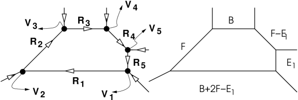
Refer to caption
Figure 16: 5-brane web of the local F2subscript𝐹2F_{2} blown-up at one point.
𝒱1=T1S1,𝒱2=TS1,𝒱3=S1T1,𝒱4=T1S1,𝒱5=TS1.formulae-sequencesubscript𝒱1superscript𝑇1superscript𝑆1formulae-sequencesubscript𝒱2𝑇superscript𝑆1formulae-sequencesubscript𝒱3superscript𝑆1superscript𝑇1formulae-sequencesubscript𝒱4superscript𝑇1superscript𝑆1subscript𝒱5𝑇superscript𝑆1\displaystyle{\cal V}_{1}=T^{-1}S^{-1}\,,\,\,{\cal V}_{2}=TS^{-1}\,,\,{\cal V}_{3}=S^{-1}T^{-1}\,,\,{\cal V}_{4}=T^{-1}S^{-1}\,,\,{\cal V}_{5}=TS^{-1}\,. (95)

The amplitude is given by,

eFinst(c)=a=15Raeb=15lbrbb=15Rb+1|𝒱b+1|Rb.superscript𝑒subscriptsuperscript𝐹𝑐𝑖𝑛𝑠𝑡superscriptsubscript𝑎15subscriptsubscript𝑅𝑎superscript𝑒superscriptsubscript𝑏15subscript𝑙𝑏subscript𝑟𝑏superscriptsubscriptproduct𝑏15quantum-operator-productsubscript𝑅𝑏1subscript𝒱𝑏1subscript𝑅𝑏\displaystyle e^{F^{(c)}_{inst}}=\sum_{a=1}^{5}\sum_{R_{a}}e^{-\sum_{b=1}^{5}l_{b}r_{b}}\prod_{b=1}^{5}\langle R_{b+1}|{\cal V}_{b+1}|R_{b}\rangle\,. (96)

Where R6=R1subscript𝑅6subscript𝑅1R_{6}=R_{1} and 𝒱6=𝒱1subscript𝒱6subscript𝒱1{\cal V}_{6}={\cal V}_{1}. By calculating the terms with la=δabsubscript𝑙𝑎subscript𝛿𝑎𝑏l_{a}=\delta_{ab} we can determine the renormalized; Kähler parameters in terms of rbsubscript𝑟𝑏r_{b},

r1subscript𝑟1\displaystyle r_{1} =\displaystyle= TB+2TFTE1+log(λ),subscript𝑇𝐵2subscript𝑇𝐹subscript𝑇subscript𝐸1log𝜆\displaystyle T_{B}+2T_{F}-T_{E_{1}}+\mbox{log}(\lambda)\,, (97)
r2subscript𝑟2\displaystyle r_{2} =\displaystyle= TF+log(λ),subscript𝑇𝐹log𝜆\displaystyle T_{F}+\mbox{log}(\lambda)\,,
r3subscript𝑟3\displaystyle r_{3} =\displaystyle= TB+log(λ),subscript𝑇𝐵log𝜆\displaystyle T_{B}+\mbox{log}(\lambda)\,,
r4subscript𝑟4\displaystyle r_{4} =\displaystyle= TFTE1+log(λ),subscript𝑇𝐹subscript𝑇subscript𝐸1log𝜆\displaystyle T_{F}-T_{E_{1}}+\mbox{log}(\lambda)\,,
r5subscript𝑟5\displaystyle r_{5} =\displaystyle= TE1+log(λ).subscript𝑇subscript𝐸1log𝜆\displaystyle T_{E_{1}}+\mbox{log}(\lambda)\,.

In terms of the renormalized Kähler parameters the amplitude is given by,

eFinst(c)=a=15Rae(lBTBlFTFlE1TE1)(1)l1+l4+l5q12(κR5κR4κR1)b=15𝒲Rb+1,Rb.superscript𝑒subscriptsuperscript𝐹𝑐𝑖𝑛𝑠𝑡superscriptsubscript𝑎15subscriptsubscript𝑅𝑎superscript𝑒subscript𝑙𝐵subscript𝑇𝐵subscript𝑙𝐹subscript𝑇𝐹subscript𝑙subscript𝐸1subscript𝑇subscript𝐸1superscript1subscript𝑙1subscript𝑙4subscript𝑙5superscript𝑞12subscript𝜅subscript𝑅5subscript𝜅subscript𝑅4subscript𝜅subscript𝑅1superscriptsubscriptproduct𝑏15subscript𝒲subscript𝑅𝑏1subscript𝑅𝑏\displaystyle e^{F^{(c)}_{inst}}=\sum_{a=1}^{5}\sum_{R_{a}}\,e^{-(l_{B}T_{B}-l_{F}T_{F}-l_{E_{1}}T_{E_{1}})}\,(-1)^{l_{1}+l_{4}+l_{5}}\,q^{\frac{1}{2}(\kappa_{R_{5}}-\kappa_{R_{4}}-\kappa_{R_{1}})}\prod_{b=1}^{5}{\cal W}_{R_{b+1},R_{b}}\,. (98)

where

lB:=l1+l3,lF:=2l1+l2+l4,lE1=l1+l4l5.formulae-sequenceassignsubscript𝑙𝐵subscript𝑙1subscript𝑙3formulae-sequenceassignsubscript𝑙𝐹2subscript𝑙1subscript𝑙2subscript𝑙4subscript𝑙subscript𝐸1subscript𝑙1subscript𝑙4subscript𝑙5\displaystyle l_{B}:=l_{1}+l_{3}\,,\,\,l_{F}:=2l_{1}+l_{2}+l_{4}\,,\,\,l_{E_{1}}=l_{1}+l_{4}-l_{5}\,. (99)

We compute the invariants for exceptional curves E1subscript𝐸1E_{1} and FE1𝐹subscript𝐸1F-E_{1} to show that the amplitude gives the correct result.

E1subscript𝐸1E_{1}: Only one term with (l1,l2,l3,l4,l5)=(0,0,0,0,1)subscript𝑙1subscript𝑙2subscript𝑙3subscript𝑙4subscript𝑙500001(l_{1},l_{2},l_{3},l_{4},l_{5})=(0,0,0,0,1) contributes,

(E1)subscript𝐸1\displaystyle{\cal I}(E_{1}) =\displaystyle= eTE1(1)𝒲 2,superscript𝑒subscript𝑇subscript𝐸11subscriptsuperscript𝒲2 \displaystyle e^{-T_{E_{1}}}(-1){\cal W}^{2}_{\vbox{\offinterlineskip\kern 1.0pt\hbox{\kern 1.0pt\vbox{\hbox{\noindent\vbox{\hbox{\vbox to0.0pt{\hrule height=0.4pt,width=3.90555pt\vss}}\hbox{\vbox{\hbox to0.0pt{\vrule width=0.4pt,height=3.90555pt\hss}}\kern 3.90555pt\vbox{\hbox to0.0pt{\vrule width=0.4pt,height=3.90555pt\hss}}}\hbox{\vbox{\hbox{\vbox to0.0pt{\hrule height=0.4pt,width=4.30554pt\vss}}}\kern-0.4pt}}}\hbox{}}\kern 1.0pt\kern 0.4pt}\kern 1.0pt\kern 0.4pt}}\,,
=\displaystyle= eTE1(2sin(gs/2))2NE1g=δg,0.\displaystyle\frac{e^{-T_{E_{1}}}{(2\mbox{sin}(g_{s}/2))^{2}}}{\,}\mapsto\,\,\,\,\,\,N^{g}_{E_{1}}=\delta_{g,0}\,.

FE1𝐹subscript𝐸1F-E_{1}: In this case also only one term with la=δa,4subscript𝑙𝑎subscript𝛿𝑎4l_{a}=\delta_{a,4} contributes,

(FE1)𝐹subscript𝐸1\displaystyle{\cal I}(F-E_{1}) =\displaystyle= e(TFTE1)(1)𝒲 2,superscript𝑒subscript𝑇𝐹subscript𝑇subscript𝐸11subscriptsuperscript𝒲2 \displaystyle e^{-(T_{F}-T_{E_{1}})}\,(-1)\,{\cal W}^{2}_{\vbox{\offinterlineskip\kern 1.0pt\hbox{\kern 1.0pt\vbox{\hbox{\noindent\vbox{\hbox{\vbox to0.0pt{\hrule height=0.4pt,width=3.90555pt\vss}}\hbox{\vbox{\hbox to0.0pt{\vrule width=0.4pt,height=3.90555pt\hss}}\kern 3.90555pt\vbox{\hbox to0.0pt{\vrule width=0.4pt,height=3.90555pt\hss}}}\hbox{\vbox{\hbox{\vbox to0.0pt{\hrule height=0.4pt,width=4.30554pt\vss}}}\kern-0.4pt}}}\hbox{}}\kern 1.0pt\kern 0.4pt}\kern 1.0pt\kern 0.4pt}}\,,
=\displaystyle= e(TFTE1)(2sin(gs/2))2,NFE1g=δg,0.\displaystyle\frac{e^{-(T_{F}-T_{E_{1}})}}{(2\mbox{sin}(g_{s}/2))^{2}}\,,\,\mapsto\,\,\,\,N^{g}_{F-E_{1}}=\delta_{g,0}\,.

5.8 F2subscript𝐹2F_{2} blown-up at two points

The web diagram is shown in Fig. 17 from which we obtain the following SL(2,𝖹𝖹)𝑆𝐿2𝖹𝖹SL(2,{\sf Z\!\!\!Z}) matrices associated with the vertices

Refer to caption
Figure 17: 5-brane web dual to the local F2subscript𝐹2F_{2} blown-up at two points.
𝒱1=T1S1,𝒱2=𝒱3=𝒱4=S1T1,𝒱5=𝒱6=T1S1.formulae-sequenceformulae-sequencesubscript𝒱1superscript𝑇1superscript𝑆1subscript𝒱2subscript𝒱3subscript𝒱4superscript𝑆1superscript𝑇1subscript𝒱5subscript𝒱6superscript𝑇1superscript𝑆1\displaystyle{\cal V}_{1}=T^{-1}S^{-1}\,,\,\,{\cal V}_{2}={\cal V}_{3}={\cal V}_{4}=S^{-1}T^{-1}\,,\,\,{\cal V}_{5}={\cal V}_{6}=T^{-1}S^{-1}\,. (102)

The amplitude is then given by,

eFinst(c)=a=16Raeb=16lbrbb=16Rb+1|𝒱b+1|Rb.superscript𝑒subscriptsuperscript𝐹𝑐𝑖𝑛𝑠𝑡superscriptsubscript𝑎16subscriptsubscript𝑅𝑎superscript𝑒superscriptsubscript𝑏16subscript𝑙𝑏subscript𝑟𝑏superscriptsubscriptproduct𝑏16quantum-operator-productsubscript𝑅𝑏1subscript𝒱𝑏1subscript𝑅𝑏\displaystyle e^{F^{(c)}_{inst}}=\sum_{a=1}^{6}\sum_{R_{a}}e^{-\sum_{b=1}^{6}l_{b}r_{b}}\prod_{b=1}^{6}\langle R_{b+1}|{\cal V}_{b+1}|R_{b}\rangle\,. (103)

Where R7=R1subscript𝑅7subscript𝑅1R_{7}=R_{1} and 𝒱7=𝒱1subscript𝒱7subscript𝒱1{\cal V}_{7}={\cal V}_{1}. By calculating the terms with la=δabsubscript𝑙𝑎subscript𝛿𝑎𝑏l_{a}=\delta_{ab} we can determine the renormalized Kähler parameters in terms of rbsubscript𝑟𝑏r_{b},

r1subscript𝑟1\displaystyle r_{1} =\displaystyle= TB+2TFTE1TE2+log(λ),subscript𝑇𝐵2subscript𝑇𝐹subscript𝑇subscript𝐸1subscript𝑇subscript𝐸2log𝜆\displaystyle T_{B}+2T_{F}-T_{E_{1}}-T_{E_{2}}+\mbox{log}(\lambda)\,, (104)
r2subscript𝑟2\displaystyle r_{2} =\displaystyle= TE2+log(λ),subscript𝑇subscript𝐸2log𝜆\displaystyle T_{E_{2}}+\mbox{log}(\lambda)\,,
r3subscript𝑟3\displaystyle r_{3} =\displaystyle= TFTE2+log(λ),subscript𝑇𝐹subscript𝑇subscript𝐸2log𝜆\displaystyle T_{F}-T_{E_{2}}+\mbox{log}(\lambda)\,,
r4subscript𝑟4\displaystyle r_{4} =\displaystyle= TB+log(λ),subscript𝑇𝐵log𝜆\displaystyle T_{B}+\mbox{log}(\lambda)\,,
r5subscript𝑟5\displaystyle r_{5} =\displaystyle= TFTE1+log(λ),subscript𝑇𝐹subscript𝑇subscript𝐸1log𝜆\displaystyle T_{F}-T_{E_{1}}+\mbox{log}(\lambda)\,,
r6subscript𝑟6\displaystyle r_{6} =\displaystyle= TE1+log(λ).subscript𝑇subscript𝐸1log𝜆\displaystyle T_{E_{1}}+\mbox{log}(\lambda)\,.

In terms of TB,F,E1,E2subscript𝑇𝐵𝐹subscript𝐸1subscript𝐸2T_{B,F,E_{1},E_{2}} the amplitude is given by

eFinst(c)=a=16Rae(lBTB+lFTFlE1TE1lE2TE2)(1)l2+l3+l5+l6q12(2κR1+κR2+κR3+κR5+κR6)b=16𝒲Rb+1,Rb.superscript𝑒subscriptsuperscript𝐹𝑐𝑖𝑛𝑠𝑡superscriptsubscript𝑎16subscriptsubscript𝑅𝑎superscript𝑒subscript𝑙𝐵subscript𝑇𝐵subscript𝑙𝐹subscript𝑇𝐹subscript𝑙subscript𝐸1subscript𝑇subscript𝐸1subscript𝑙subscript𝐸2subscript𝑇subscript𝐸2superscript1subscript𝑙2subscript𝑙3subscript𝑙5subscript𝑙6superscript𝑞122subscript𝜅subscript𝑅1subscript𝜅subscript𝑅2subscript𝜅subscript𝑅3subscript𝜅subscript𝑅5subscript𝜅subscript𝑅6superscriptsubscriptproduct𝑏16subscript𝒲subscript𝑅𝑏1subscript𝑅𝑏\displaystyle e^{F^{(c)}_{inst}}=\sum_{a=1}^{6}\sum_{R_{a}}e^{-(l_{B}T_{B}+l_{F}T_{F}-l_{E_{1}}T_{E_{1}}-l_{E_{2}}T_{E_{2}})}\,(-1)^{l_{2}+l_{3}+l_{5}+l_{6}}\,q^{-\frac{1}{2}(2\kappa_{R_{1}}+\kappa_{R_{2}}+\kappa_{R_{3}}+\kappa_{R_{5}}+\kappa_{R_{6}})}\,\prod_{b=1}^{6}{\cal W}_{R_{b+1},R_{b}}\,.

where

lB:=l1+l4,lF:=2l1+l3+l5,lE1:=l1+l5l6lE2:=l1+l3l2.formulae-sequenceassignsubscript𝑙𝐵subscript𝑙1subscript𝑙4formulae-sequenceassignsubscript𝑙𝐹2subscript𝑙1subscript𝑙3subscript𝑙5assignsubscript𝑙subscript𝐸1subscript𝑙1subscript𝑙5subscript𝑙6subscript𝑙subscript𝐸2assignsubscript𝑙1subscript𝑙3subscript𝑙2\displaystyle l_{B}:=l_{1}+l_{4}\,,\,\,l_{F}:=2l_{1}+l_{3}+l_{5}\,,\,\,l_{E_{1}}:=l_{1}+l_{5}-l_{6}\,\,\,l_{E_{2}}:=l_{1}+l_{3}-l_{2}\,. (105)

6 Conclusions

We have seen that topological closed string amplitudes can be written down directly from the web diagram although underlying reason for a such a simple description of these amplitudes is still a mystery. It would be extremely interesting to find this underlying theory giving the propagator and the three point vertex not only because it would give important insight into closed string amplitudes but it may also provide a simple way of computing all genus open string amplitudes. We believe that open string amplitudes also have a similar description in terms of 5-brane webs with extra ingredient that we insert an operator in the calculation of amplitude corresponding to the 3-cycle on which the holomorphic curves can have boundaries as discussed in [37, 38].

Refer to caption
Figure 18: Dashed line represents the non-compact 3-cycles on which D6-brane is wrapped.

Acknowledgments

I would like to thank Jacques Distler, Vadim Kaplunovsky and Cumrun Vafa for valuable discussions. This research was supported by NSF grant PHY-0071512.

References

  • [1] M. Bershadsky, S. Cecotti, H. Ooguri, C. Vafa, “Kodaira-Spencer Theory of Gravity and Exact Results for Quantum String Amplitudes,” Commun. Math. Phys. 165 (1994) 311-428.
  • [2] M. Gromov, “ Pseudo-holomorphic Curves on Almost Complex Manifolds,” Invent. Math. 82 (1985) 307-347.
  • [3] E. Witten, “Topological Sigma Models,” Commun. Math. Phys. 118 (1988) 411-449.
  • [4] P. S. Aspinwall, D. Morrison, “Topological Field Theory and Rational Curves,” Commun. Math. Phys. 151 (1993) 245-262, hep-th/9110048.
  • [5] E. Witten, “Mirror Manifolds and Topological Field Theory,” hep-th/9112056.
  • [6] T. -M. Chiang, A. Klemm, S. -T. Yau, E. Zaslow, “Local Mirror Symmetry: Calculation and Interpretations,” Adv. Theor. Math. Phys. 3 (1999) 495-565, hep-th/9903053.
  • [7] A. Klemm, E. Zaslow, “Local Mirror Symmetry at Higher Genus,” hep-th/9906046.
  • [8] D. Ghoshal, C.Vafa, “c=1 String as the Topological Theory of the Conifold,” Nucl. Phys. B453 121-128, hep-th9506122.
  • [9] S. Katz, A. Klemm, C. Vafa, “M-Theory, Topological Strings and Spinning Black Holes,” Adv. Theor. Math. Phys. 3 (1999) 1445-1537, hep-th/9910181.
  • [10] R. Gopakumar, C. Vafa, “M-Theory and topological strings-II,” hep-th/9812127.
  • [11] H. Ooguri, C. Vafa, “Knot invariants and topological strings,” Nucl. Phys. B 577 (2000) 419, hep-th/9912123.
  • [12] R. Gopakumar, C. Vafa, “On the gauge theory/geometry correspondence,” Adv. Theor. Math. Phys. 3 (1999) 1415, hep-th/9811131.
  • [13] H. Ooguri, C. Vafa, “Worldsheet Derivation of a Large N𝑁N Duality,” hep-th/0205297.
  • [14] J. M. F. Labastida, M. Mariño, “Polynomial invariants for torus knots and topological strings,” Commun. Math. Phys. 217 (2001) 423-449, hep-th/0004196.
  • [15] P. Ramadevi, T. Sarkar, “On Link Invariants and Topological String Amplitudes,” Nucl. Phys. B600 (2001) 487-511, hep-th/0009188.
  • [16] J. M. F. Labastida, M. Mariño, C. Vafa, “Knots, links and branes at large N,” JHEP 0011 (2000) 007, hep-th/0010102.
  • [17] S. Sinha, C. Vafa, “SO and Sp Chern-Simons at large N,” hep-th/0012136.
  • [18] A. Iqbal, A. -K. Kashani-Poor, in progress.
  • [19] M. Mariño, C. Vafa, “Framed knots at large N,” hep-th/0108064.
  • [20] D. -E. Diaconescu, B. Florea, A. Grassi, “Geometric Transitions and Open String Instantons,” hep-th/0205234;
    D. -E. Diaconescu, B. Florea, A. Grassi, “Geometric transitions, del Pezzo surfaces and open string instantons,” hep-th/0206163.
  • [21] M. Aganagic, M. Mariño, C. Vafa, ”All Loop Topological String Amplitudes From Chern-Simons Theory”, hep-th/0206164.
  • [22] E. Witten, “Chern-Simons gauge theory as a string theory,” in The Floer memorial volume, Birkhäuser 1995, p.637, hep-th/9207094.
  • [23] N. C. Leung, C. Vafa, “Branes and Toric Geometry,” Adv. Theor. Math. Phys. 2 (1998) 91-118, hep-th/9711013.
  • [24] O. DeWolfe, A. Hanany, A. Iqbal, E. Katz, “Five-branes, Seven-branes and Five-dimensional Ensubscript𝐸𝑛E_{n} field theories,” JHEP 9903 (1999) 006, hep-th/9902179.
  • [25] O. Aharony, A. Hanany, B. Kol, “Webs of (p,q) 5-branes, Five Dimensional Field Theories and Grid Diagrams,” JHEP 9801 (1998) 002, hep-th/9710116.
  • [26] B. Kol, J. Rahmfeld, “BPS Spectrum of 5 Dimensional Field Theories, (p,q) Webs and Curve Counting,” JHEP 9808 (1998) 006, hep-th/9801067.
  • [27] G. Bonelli, “The M5-brane on K3 and del Pezzo’s and multi-loop string amplitudes,” JHEP 0112 (2001) 022, hep-th/0111126.
  • [28] R. Dijkgraaf, E. Verlinde, M. Vonk, “On the partition sum of the NS five-brane,” hep-th/0205281.
  • [29] K. Hori, C. Vafa, “Mirror Symmetry,” hep-th/0002222,
  • [30] K. Hori, A. Iqbal, C. Vafa, “D-branes and Mirror Symmetry,” hep-th/0005247.
  • [31] E. Witten, “Phases of N=2𝑁2N=2 Theories In Two Dimensions,” Nucl. Phys. B403 (1993) 159-222, hep-th/9301042.
  • [32] E. Verlinde, “Fusion rules and modular transformations in 2-D conformal field theory,” Nucl. Phys. B 300 (1988) 360.
  • [33] M. Aganagic, D. -E. Diaconescu, A. Grassi, M. Mariño, C. Vafa, To appear.
  • [34] E. Witten, “Quantum field theory and the Jones polynomial,” Commun. Math. Phys. 121 (1989) 351.
  • [35] H. R. Morton, S. G. Lukac, “The HOMFLY polynomial of the decorated Hopf link,” math.GT/0108011.
  • [36] S. G. Lukac, “HOMFLY skeins and the Hopf link,” Ph.D Thesis, June 2001, in http://www.liv.ac.uk/ su14/knotgroup.html
  • [37] M. Aganagic, C. Vafa, “Mirror Symmetry, D-Branes and Counting Holomorphic Discs,” hep-th/0012941.
  • [38] M. Aganagic, A. Klemm, C. Vafa, “Disk instantons, mirror symmetry and the duality web,” Z. Naturforsch. A 57 (2002) 1, hep-th/0105045.