Towards Field Theory in Spaces with Multivolume Junctions

Abstract

We consider a spacetime formed by several pieces having common timelike boundary which plays the role of a junction between them. We establish junction conditions for fields of various spin and derive the resulting laws of wave propagation through the junction, which turn out to be quite similar for fields of all spins. As an application, we consider the case of multivolume junctions in four-dimensional spacetime that may arise in the context of the theory of quantum creation of a closed universe on the background of a big mother universe. The theory developed can also be applied to braneworld models and to the superstring theory.

I Introduction

In this paper, we consider field theory on spaces with the so-called multivolume junctions, as shown in Fig. 1. Spaces of such topological configurations arise in several important contexts. Firstly, they arise in the study of various braneworld theories that became very popular after the seminal papers RS . In these theories, the dimensionality of the volume spaces is usually equal to five, and the junction, which is called brane, is four-dimensional and is identified with the physical spacetime. Normally, the brane in a braneworld theory separates two volume spaces; the corresponding situation is shown in Fig. 2. However, the brane may be a junction of more than two volume spaces as well as it may be a boundary of only one volume space. Thus, in CS , junctions of an arbitrary number of semi-infinite four-branes were under consideration, and the whole configuration was assumed to be embedded in a six-dimensional spacetime. Secondly, such spaces may represent the situation where the physical four-dimensional spacetime has a nontrivial topology of the type shown in Fig. 1. Thirdly, in the important case of two-dimensional volume spaces, our investigation may be applicable to the superstring theory. Note that three-volume junctions of boson strings of type shown in Fig. 1 were under consideration in string .

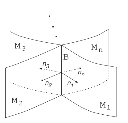
Figure 1: Multivolume junction.

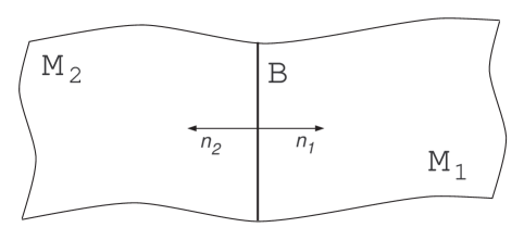
Figure 2: Two-volume junction.

In this paper, we consider the general situation depicted in Fig. 1. It symbolically shows $n$ $d$-dimensional Lorentzian manifolds ${\mathcal{M}}_{s}$, $s=1,\ldots,n$, with common $(d\!-\!1)$-dimensional boundary ${\mathcal{B}}$ which thus plays the role of a junction between them. The boundary ${\mathcal{B}}$ is assumed to be timelike, so that all the respective inner normal vector fields $n^{a}_{(s)}$, $s=1,\ldots,n$, at this boundary are spacelike. We do not consider the space of Fig. 1 as embedded in a higher-dimensional manifold. Our aim is to study the behavior of various fields in a space with the specified topology focussing attention on the derivation and analysis of the junction conditions at ${\mathcal{B}}$.

In brane theories, together with fields in the volume, one also considers fields whose dynamics is restricted to the brane RS . Moreover, the action for the brane may involve the restrictions of some of the volume fields to the brane; for example, it typically involves the induced metric. However, in this paper, we restrict ourselves mainly to the case where the junction ${\mathcal{B}}$ does not have its intrinsic dynamics and thus represents what might be called a generalization of an imaginary hypersurface separating two volumes in an ordinary space to the case where the number of volumes is greater than two.

As a concrete example of application of our theory, we consider the case of multivolume junctions in a four-dimensional spacetime (Sec. VII). The issue of such a junction may arise in the context of the theory of quantum creation of a closed universe on the background of a big mother universe Fomin . It is conceivable that the created baby universe does not become spatially separated from the mother universe, but rather remains glued with it over some common three-dimensional volume FSB . The corresponding situation is depicted in Fig. 3, which shows the mother universe ${\mathcal{M}}_{1}$ and the baby universe ${\mathcal{M}}_{2}$ glued over the volume ${\mathcal{M}}_{3}$. All the three volume regions ${\mathcal{M}}_{1}$, ${\mathcal{M}}_{2}$, and ${\mathcal{M}}_{3}$ may evolve metrically preserving the topological configuration as shown in Fig. 3. One of the important physical questions in this situation is the issue of the behavior of various physical fields in this topology, in particular, the conditions of propagation of waves through the junction ${\mathcal{B}}$ which is the common boundary of all three volume regions.

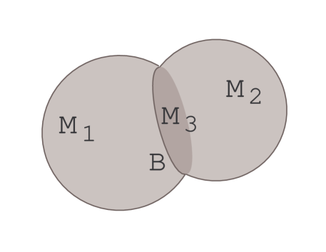
Figure 3: Closed universe with multivolume junctions.

In approaching this issue, we first establish junction conditions for fields of various spins (Secs. II–IV) and then consider the resulting laws of wave propagation through the junction ${\mathcal{B}}$ (Sec. V). In principle, the junction conditions at ${\mathcal{B}}$ may be specified in many different ways. However, with a natural requirement that the spaces ${\mathcal{M}}_{s}$ be treated identically, it turns out that there are precisely two versions of junction conditions for each spin. This is one of the reasons why we pay attention to spaces with the topology specified above and propose to study them in greater detail.

In Sec. VI, we study the Green functions in the case of junction of flat spaces over a flat boundary and the resulting quantum vacuum stress-energy tensor.

Concluding remarks are presented in Sec. VIII.

II Junction conditions for the metric

We start with considering junction conditions for the metric because the actions for all other fields involve ingredients (for example, the volume element) associated with the metric. In this paper, we consider the metric $g_{ab}$ with signature $+--\ldots-$. The general action for the metric can be written in the form GH

$$S=-M^{d-2}\left(\int_{\mathcal{M}}R+2\sum_{s}\int_{\mathcal{B}}K^{(s)}\right)+\int_{\mathcal{B}}L_{h}\,,$$ (1)

where $M$ is the Planck mass, $R$ is the scalar curvature, and $K^{(s)}$ is the trace of the extrinsic curvature of the junction ${\mathcal{B}}$ in the space ${\mathcal{M}}_{s}$. We impose the most natural junction conditions for the metric, namely, that the induced metric $h_{ab}$ on ${\mathcal{B}}$ is one and the same in all the spaces ${\mathcal{M}}_{s}$, $s=1,\ldots,n$. The Lagrangian $L_{h}$ in (1) depends only on this induced metric.

In this paper, we use the notation and conventions of Wald . The extrinsic curvature and its trace are defined as follows:

$$K_{ab}=h^{c}{}_{a}\nabla_{c}n_{b}\,,\quad K=K_{ab}h^{ab}\,,$$ (2)

where $h_{ab}=g_{ab}+n_{a}n_{b}$ is the metric induced on a timelike hypersurface. The natural volume elements are implied in all the integrations over ${\mathcal{M}}$ and ${\mathcal{B}}$. The cosmological-constant terms can be added to action (1) for each space ${\mathcal{M}}_{s}$, and their contribution to the resulting equations is obvious.

Variation of action (1) can be written in the form (see Appendix)

$$\delta S=-M^{d-2}\left[\int_{\mathcal{M}}G_{ab}\delta g^{ab}+\int_{\mathcal{B}}\sum_{s}\left(K_{ab}^{(s)}-K^{(s)}h_{ab}\right)\delta h^{ab}\right]+\int_{\mathcal{B}}\sigma_{ab}\delta h^{ab}\,.$$ (3)

Here, $G_{ab}$ is the Einstein tensor, $\sigma_{ab}$ is the variation of the last term in (1) with respect to $h^{ab}$, and the variation $\delta h^{ab}$ is completely determined by the variation $\delta g^{ab}$ of the metric in ${\mathcal{M}}$. Note that the Gibbons–Hawking boundary terms GH in action (1) are required to consistently obtain the Einstein equations in the respective volume spaces without restricting variations of the metric at the junction ${\mathcal{B}}$.

Besides the metric, we may have additional fields $\Phi$ that propagate in the volume and fields $\varphi$ whose dynamics is restricted to the junction. Some of the fields $\varphi$ may represent restrictions of some of the volume fields $\Phi$ to the junction. Thus, in general, we must consider the action for the fields with the corresponding Lagrangians $L_{\Phi}$ and $L_{\varphi}$ in the form

$$\int_{\mathcal{M}}L_{\Phi}+\int_{\mathcal{B}}L_{\varphi}\,.$$ (4)

The additional set of junction conditions obtained with the account of (3), (4) is then

$$\sum_{s}\left(K_{ab}^{(s)}-K^{(s)}h_{ab}\right)={1\over M^{d-2}}\left(\sigma_{ab}+\tau_{ab}\right)\,,$$ (5)

where $\tau_{ab}$ is the variation of (4) with respect to the induced metric $h^{ab}$.

Variation of the first term in (4), together with (3), leads to the Einstein equation in the volume

$$G_{ab}={1\over M^{d-2}}\,T_{ab}\,,$$ (6)

where $T_{ab}$ is the variation of the first term in (4) with respect to the metric $g^{ab}$.

III Junction conditions for scalar and vector fields

A complex scalar field $\phi$ with mass $m$ is described by the action

$$S=\int_{\mathcal{M}}\left[\overline{\nabla_{a}\phi}\nabla^{a}\phi-m^{2}\bar{\phi}\phi\right]\,,$$ (7)

where the bar denotes complex conjugation, the integral is taken over the whole manifold ${\mathcal{M}}=\cup_{s}{\mathcal{M}}_{s}$ shown in Fig. 1, and the natural volume element is implied. The derivative $\nabla_{a}\phi$ may involve contribution from the gauge vector field.

In formulating the junction conditions at ${\mathcal{B}}$, we proceed from the following natural principles. Let $\phi_{(s)}$ denote the restriction of the scalar field $\phi$ to the space ${\mathcal{M}}_{s}$. We are going to relate the value of $\phi_{(s)}$ with the values of $\phi_{(r)}$, $r\neq s$ at the junction. This relation must be linear (in order to respect the superposition principle), and the spaces ${\mathcal{M}}_{s}$ must be regarded as physically identical. With these requirements, we arrive at the following general junction conditions at ${\mathcal{B}}$:

$$\phi_{(s)}=\alpha\sum_{r\neq s}\phi_{(r)}\,,\quad s=1,\ldots,n\,,$$ (8)

where $\alpha$ is some constant to be determined. Possible values of $\alpha$ are obtained from the additional requirement that the junction conditions (8) allow for nontrivial solutions at the junction. This gives only two possible values of the parameter $\alpha$:

$$\alpha={1\over n-1}\quad\mbox{and}\quad\alpha=-1\,.$$ (9)

Notably, the condition $\alpha=1/(n-1)$ simply implies the continuity of the scalar field in the space ${\mathcal{M}}=\cup_{s}{\mathcal{M}}_{s}$, i.e., the condition $\phi_{(1)}=\phi_{(2)}=\cdots=\phi_{(n)}$, while the condition $\alpha=-1$ leads to the single equation $\sum_{s}\phi_{(s)}=0$. To obtain other conditions at the junction, we vary the action respecting the junction conditions (8) and demanding that the variation be zero. General variation of action (7) is given by

$$\begin{array}[]{ll}\delta S=&\displaystyle-\int_{\mathcal{M}}\left[\delta\bar{\phi}\left(\nabla^{a}\nabla_{a}+m^{2}\right)\phi+\delta\phi\left(\bar{\nabla}^{a}\bar{\nabla}_{a}+m^{2}\right)\bar{\phi}\right]\vskip 6.0pt plus 2.0pt minus 2.0pt\\ &\displaystyle+\sum_{s}\int_{\mathcal{B}}\left(\delta\bar{\phi}_{(s)}\nabla_{a}\phi_{(s)}+\delta\phi_{(s)}\bar{\nabla}_{a}\bar{\phi}_{(s)}\right)n^{a}_{(s)}\,.\end{array}$$ (10)

According to the value of $\alpha$ in (8), we obtain, besides the Klein–Gordon equations of motion in the volume, also the additional junction conditions.

A. Case of $\alpha=1/(n-1)$

In this case, the additional junction conditions are $\sum_{s}n^{a}_{(s)}\nabla_{a}\phi_{(s)}=0$. We summarize the junction conditions obtained in the case under consideration:

$$\phi_{(p)}=\phi_{(q)}\quad\mbox{for all $p,q$}\,;\quad\sum_{s}n^{a}_{(s)}\nabla_{a}\phi_{(s)}=0\,.$$ (11)

B. Case of $\alpha=-1$

In this case, the complete set of junction conditions is

$$\sum_{s}\phi_{(s)}=0\,;\quad n^{a}_{(p)}\nabla_{a}\phi_{(p)}=n^{a}_{(q)}\nabla_{a}\phi_{(q)}\quad\mbox{for all $p,q$}\,.$$ (12)

Both sets of junction conditions (11) and (12) imply the sum rule for the components of the conserved current $J_{a}=i\left(\bar{\phi}\nabla_{a}\phi-\phi\bar{\nabla}_{a}\bar{\phi}\right)$ normal to the junction surface ${\mathcal{B}}$:

$$\sum_{s}n^{a}_{(s)}J_{a}^{(s)}=0\,.$$ (13)

The junction conditions (11) also imply that the components of the current along the junction surface ${\mathcal{B}}$ are the same in all the volume spaces.

A free vector field $A^{a}$ with mass $m$ is described by the action

$$S=\int_{\mathcal{M}}\left(-\frac{1}{4}F_{ab}F^{ab}+{m^{2}\over 2}A_{a}A^{a}\right)\,.$$ (14)

Its variation in the manifold ${\mathcal{M}}$ is given by

$$\delta S=-\int_{\mathcal{M}}\delta A_{b}\left(\nabla_{a}F^{ab}+m^{2}A^{b}\right)-\sum_{s}\int_{\mathcal{B}}\delta A_{b}^{(s)}F^{ab}_{(s)}n_{a}^{(s)}\,.$$ (15)

The junction conditions at ${\mathcal{B}}$ naturally will involve only the components of $A^{a}$ tangent to ${\mathcal{B}}$, which we denote by $A^{\parallel a}$. Similarly to Eq. (8), we write the most general expression compatible with the symmetry imposed:

$$A^{\parallel a}_{(s)}=\alpha\sum_{r\neq s}A^{\parallel a}_{(r)}\,,\ \ s=1,\ldots,n\,,$$ (16)

where, by reasoning similar to that of the scalar case, the constant $\alpha$ is equal either to $1/(n-1)$ or to $-1$.

A. Case of $\alpha=1/(n-1)$

In this case, the values of $A^{\parallel a}$ are the same at all the sides of the junction ${\mathcal{B}}$. Variation of action (15) yields the Proca equations (the Maxwell equations, if $m=0$) in the volume and the additional junction conditions $\sum_{s}F^{ab}_{(s)}n^{(s)}_{b}=0$. We summarize the junction conditions in this case:

$$A^{\parallel a}_{(p)}=A^{\parallel a}_{(q)}\quad\mbox{for all $p,q$}\,;\quad\sum_{s}F^{ab}_{(s)}n^{(s)}_{b}=0\,.$$ (17)

B. Case of $\alpha=-1$

In this case, the total set of junction conditions obtained with the account of (15) is given by

$$\sum_{s}A^{\parallel a}_{(s)}=0\,;\quad F^{ab}_{(p)}n^{(p)}_{b}=F^{ab}_{(q)}n^{(q)}_{b}\quad\mbox{for all $p,q$}\,.$$ (18)

In the case $n=1$, i.e., where there is only one volume space with boundary, the junction conditions of type A [Eqs. (11), (17)] become the Neumann boundary conditions, while the junction conditions of type B [Eqs. (12), (18)] become the Dirichlet boundary conditions. Thus, the junction conditions obtained above can be regarded as respective generalizations of the mentioned boundary conditions to the case of $n>1$.

IV Junction conditions for the Dirac field

The action for the Dirac field of mass $m$ can be written in the form

$$S=\int_{\mathcal{M}}\left({i\over 2}\left[\overline{\psi}\gamma^{a}\nabla_{a}\psi-\overline{(\nabla_{a}\psi)}\gamma^{a}\psi\right]-m\overline{\psi}\psi\right)\,,$$ (19)

where $\nabla_{a}\psi$ denotes the standard covariant derivative of the Dirac spinor $\psi$ that may include contribution from the gauge vector field. Variation of action (19) is given by

$$\begin{array}[]{ll}\delta S=&\displaystyle\int_{\mathcal{M}}\delta\overline{\psi}\left(i\gamma^{a}\nabla_{a}-m\right)\psi-\int_{\mathcal{M}}\left[i\overline{(\nabla_{a}\psi)}\gamma^{a}+m\overline{\psi}\right]\delta\psi\vskip 6.0pt plus 2.0pt minus 2.0pt\\ &\displaystyle{}+i\sum_{s}\int_{\mathcal{B}}\left(\overline{\psi}_{(s)}\gamma^{a}\delta\psi_{(s)}-\delta\overline{\psi}_{(s)}\gamma^{a}\psi_{(s)}\right)n_{a}^{(s)}\,,\end{array}$$ (20)

where $\psi_{(s)}$, $\overline{\psi}_{(s)}$ are the restrictions of the spinor fields to the space ${\mathcal{M}}_{s}$.

The specific feature of the spinor field is that it is referred at each point to a particular orthonormal basis (called tetrad in the case of $d=4$). Thus, in order to formulate the junction conditions for the Dirac field, we must take this circumstance into account. We need to relate the spinor fields $\psi_{(s)}$, $s=1,\ldots,n$, as we reach one and the same point at the junction ${\mathcal{B}}$ moving in different spaces ${\mathcal{M}}_{s}$. At each point $x\in{\mathcal{B}}$, we must choose $n$ orthonormal bases, one in each space ${\mathcal{M}}_{s}$, $s=1,\ldots,n$, to refer the corresponding values of the Dirac field to these bases. For a convenient formulation of the relations between these values, the $n$ bases are to be chosen in a coherent way. We choose $d-1$ of the basis vectors $\{e_{1}^{a},e_{2}^{a},\ldots,e_{d-1}^{a}\}$ at any point $x\in{\mathcal{B}}$ to form an arbitrary orthonormal basis in the tangent space to ${\mathcal{B}}$, the same for all the spaces ${\mathcal{M}}_{s}$, $s=1,\ldots,n$. Then the $d$-th vector of the orthonormal basis in each space is determined uniquely up to sign, and we choose it to be the inner normal vector $n_{(s)}^{a}$, $s=1,\ldots,n$, respectively, in each of these spaces.

Next, to obtain the possible junction conditions at ${\mathcal{B}}$, we first consider the case $n=2$, i.e., a manifold ${\mathcal{M}}$ and a timelike hypersurface ${\mathcal{B}}$ that divides it into two parts ${\mathcal{M}}_{1}$ and ${\mathcal{M}}_{2}$ (see Fig. 2). Given a Dirac spinor field which is continuous in ${\mathcal{M}}$, its values at ${\mathcal{B}}$ in the bases $\{e_{1}^{a},e_{2}^{a},\ldots,e_{d-1}^{a},n_{(s)}^{a}\}$, $s=1,2$, chosen by the procedure described above are related by the operation of reflection which performs the transformation of the Dirac spinor $\psi$ from the basis $\{e_{1}^{a},e_{2}^{a},\ldots,e_{d-1}^{a},n_{(s)}^{a}\}$ to the reflected basis $\{e_{1}^{a},e_{2}^{a},\ldots,e_{d-1}^{a}$, $-n_{(s)}^{a}\}$ (since $n_{2}^{a}=-n_{1}^{a}$). For simplicity, we consider the important case where the dimensionality $d$ is even and define the corresponding matrix operator of reflection as $N=\gamma_{d+1}\gamma^{a}n_{a}$, where $\gamma_{d+1}$ is the $d$-dimensional analog of the four-dimensional $\gamma_{5}$ matrix, so that it obeys the relation $N^{2}=1$. Then we have

$$\psi_{(1)}=\pm N\psi_{(2)}\,,\quad\psi_{(2)}=\pm N\psi_{(1)}\,,$$ (21)

where the sign ambiguity corresponds to the fact that the spinor representation of the Lorentz group is double-valued.

Conditions (21) correspond to the continuity of the spinor field in the space ${\mathcal{M}}$ thus indicating that the junction ${\mathcal{B}}$ in this case is only imaginary, or nonphysical. It will be shown very soon that the junction conditions (21) may be obtained from the variational principle starting from more general conditions, namely,

$$\psi_{(1)}=(\alpha+\beta N)\psi_{(2)}\,,\quad\psi_{(2)}=(\alpha+\beta N)\psi_{(1)}\,,$$ (22)

where $\alpha$ and $\beta$ are some constants. Thus, it appears reasonable to impose the general junction conditions of the type (22) in the general case shown in Fig. 1.

We proceed with the analysis of the situation shown in Fig. 1 and impose the discussed general junction conditions at ${\mathcal{B}}$, compatible with the symmetry of the problem:

$$\psi_{(s)}=\sum_{r\neq s}\left(\alpha+\beta N\right)\psi_{(r)}\,,\quad s=1,\ldots,n\,,$$ (23)

where $\alpha$ and $\beta$ are constants.

To facilitate the analysis, we can use the decomposition $\psi=\psi^{+}+\psi^{-}$ at ${\mathcal{B}}$, where

$$\psi^{\pm}=\frac{1}{2}(1\pm N)\psi\,,\quad N\psi^{\pm}=\pm\psi^{\pm}\,.$$ (24)

Then the requirement that system (23) have nontrivial solutions both for $\psi^{+}_{(s)}$ and for $\psi^{-}_{(s)}$, $s=1,\ldots,n$, at the junction leads to the equation

$$\left[(n-1)z-1\right]\,\left(z+1\right)^{n-1}=0\,,$$ (25)

which must be satisfied both by $z=\alpha+\beta$ and by $z=\alpha-\beta$.

Two solutions of these equations for $\alpha$, $\beta$ have $\beta=0$. In this case, equation (25) implies that either $\alpha=-1$, or $\alpha=1/(n-1)$. It is easy to verify that the boundary term in the variational principle (20) in both these cases will lead to the additional condition $\psi_{(s)}=0$, $s=1,\ldots,n$, which, together with the Dirac equation in the volume, will imply vanishing of $\psi$ all over the space ${\mathcal{M}}$. Thus, the junction conditions with $\beta=0$ should be rejected as leading to only trivial solutions.

Consider the remaining two solutions with nonzero $\beta$, namely,

$$\alpha={2-n\over 2(n-1)}\,,\quad\beta=\pm{n\over 2(n-1)}\,,$$ (26)

which differ in the sign of $\beta$. By writing the fields on the junction ${\mathcal{B}}$ in the form (24) and by using the property of the reflection operator

$$N\gamma^{a}Nn_{a}=-\gamma^{a}n_{a}\,,$$ (27)

one easily can verify that both cases (26) imply the identical vanishing of the boundary term in variation (20) of the action. Thus, both cases (26) can describe the physical situation, and the possible junction conditions at ${\mathcal{B}}$ can be summarized as

$$\psi_{(s)}={1\over 2(n-1)}\sum_{r\neq s}\left[(2-n)\pm nN\right]\psi_{(r)}\,,\quad s=1,\ldots,n\,.$$ (28)

These junction conditions can be further transformed to the following convenient form:

$$(1\pm N)\psi_{(s)}={2\over n}\sum_{r}\psi_{(r)}\,,\quad s=1,\ldots,n\,.$$ (29)

In this form, the junction conditions are extended also to the case $n=1$, i.e., where ${\mathcal{B}}$ is the boundary of only one volume space; in this case, the boundary conditions imply reflection from the boundary. In the particular case of $n=2$, we obtain precisely conditions (21), which imply continuity of the Dirac field all over ${\mathcal{M}}$. As in the previous cases, we will refer to the junction conditions (29) with the upper and lower sign as to the junction conditions of type A and B, respectively, although in the case of the Dirac field, there is no qualitative difference between them.

As in the scalar case, the junction conditions (29) imply the sum rule for the components of the conserved current $J^{a}=\overline{\psi}\gamma^{a}\psi$ normal to the junction:

$$\sum_{s}J^{a}_{(s)}n^{(s)}_{a}=0\,.$$ (30)

V Wave propagation through the junction

In this section, we apply the equations obtained to the particular interesting case of wave propagation in the space shown in Fig. 1. We shall derive the laws of wave transmission through and reflection from the junction ${\mathcal{B}}$.

First, consider the simple case of a scalar field. Let, in the region ${\mathcal{M}}_{1}$, a wave that obeys the Klein–Gordon equation and propagates towards the junction ${\mathcal{B}}$ be denoted by $\phi^{(+)}_{1}$. We denote its value at ${\mathcal{B}}$ by $\phi_{\mathcal{B}}$ and its derivative normal to the junction ${\mathcal{B}}$ by $\phi^{\prime}_{\mathcal{B}}\equiv n_{(1)}^{a}\nabla_{a}\phi^{(+)}_{1}$. Then the wave which we call the reflected wave and denote by $\phi^{(-)}_{1}$ is constructed by imposing the same values at the junction, $\phi^{(-)}_{1}=\phi_{\mathcal{B}}$, and by reversing the sign of the derivative normal to the junction ${\mathcal{B}}$: $n_{(1)}^{a}\nabla_{a}\phi^{(-)}_{1}=-\phi^{\prime}_{\mathcal{B}}$. For example, in the case of propagation in a flat spacetime ${\mathcal{M}}_{1}$ with the surface ${\mathcal{B}}$ described by the equation $x_{1}=0$ in the natural spacetime coordinates $t$, $x\equiv(x_{1},x_{2},\ldots,x_{d-1})$, the plane waves of this kind will be given, respectively, by $\phi^{(+)}_{1}=\exp(-i\omega t+ik\cdot x)$ and $\phi^{(-)}_{1}=\exp(-i\omega t+ik^{\prime}\cdot x)$, where the wave vector $k^{\prime}$ is obtained from $k$ by reversing its $x_{1}$-component. The waves $\phi^{(-)}_{s}$, $s=2,\ldots,n$, propagating away from the junction, respectively, in the regions ${\mathcal{M}}_{s}$, $s=2,\ldots,n$, are constructed by imposing the boundary conditions $\phi^{(-)}_{s}=\phi_{\mathcal{B}}$, $n_{(s)}^{a}\nabla_{a}\phi^{(-)}_{s}=-\phi^{\prime}_{\mathcal{B}}$, $s=2,\ldots,n$, at the junction ${\mathcal{B}}$. We will assume that solutions with the boundary conditions imposed exist globally in ${\mathcal{M}}_{s}$, $s=1,\ldots,n$, respectively.

We are looking for a solution that contains both waves falling towards ${\mathcal{B}}$ and reflected from ${\mathcal{B}}$ in the region ${\mathcal{M}}_{1}$, but only waves propagating away from ${\mathcal{B}}$ (transmitted waves) in the regions ${\mathcal{M}}_{s}$, $s=2,\ldots,n$. Thus, we set

$$\phi_{1}=\phi^{(+)}_{1}+\rho\phi^{(-)}_{1}\,,\quad\phi_{s}=\tau_{s}\phi^{(-)}_{s}\,,\quad s=2,\ldots,n\,,$$ (31)

where $\rho$ is the amplitude of wave reflection and $\tau_{s}$ are the amplitudes of wave transmission to the spaces ${\mathcal{M}}_{s}$, $s=2,\ldots,n$, respectively.

To determine the amplitudes of reflection and transmission, we apply the junction conditions obtained in Sec. III. In the case of the junction conditions (11), we obtain

$$\left\{\begin{array}[]{l}1+\rho=\tau_{2}=\tau_{3}=\cdots=\tau_{n}\,,\\ 1-\rho-\sum_{s=2}^{n}\tau_{s}=0\,,\end{array}\right.\Longrightarrow\left\{\begin{array}[]{l}\rho=(2-n)/n\,,\\ \tau_{2}=\tau_{3}=\cdots=\tau_{n}=2/n\,.\end{array}\right.$$ (32)

In the case of the junction conditions (12), we get the solution that differs from (32) only in the sign:

$$\left\{\begin{array}[]{l}1+\rho+\sum_{s=2}^{n}\tau_{s}=0\,,\\ 1-\rho=-\tau_{2}=-\tau_{3}=\cdots=-\tau_{n}\,,\end{array}\right.\Longrightarrow\left\{\begin{array}[]{l}\rho=(n-2)/n\,,\\ \tau_{2}=\tau_{3}=\cdots=\tau_{n}=-2/n\,.\end{array}\right.$$ (33)

We see that, in both cases, the same amount of energy [the fraction $(n-2)^{2}/n^{2}$] is reflected back to the space ${\mathcal{M}}_{1}$ and the same equal amount of energy (the fraction $4/n^{2}$) is transmitted to each of the $n-1$ spaces ${\mathcal{M}}_{s}$, $s=2,\ldots,n$.

The results for the case of vector fields and for weak gravitational waves are essentially the same. For the vector field, we introduce the wave $A_{a}^{(+)}$ propagating towards the junction ${\mathcal{B}}$ in the region ${\mathcal{M}}_{1}$ and construct the reflected wave $A_{a}^{(-)}$ by keeping the component $A_{a}^{\parallel}$ tangent to ${\mathcal{B}}$ intact and by reversing the sign of the value of $F^{ab}n_{b}$ at ${\mathcal{B}}$. For a weak gravitational wave, we introduce the similar field $\delta g_{ab}^{(+)}$ and construct the corresponding reflected wave $\delta g_{ab}^{(-)}$ by keeping the perturbation of the induced metric $\delta h_{ab}$ at ${\mathcal{B}}$ intact and by reversing the sign of the perturbation of the extrinsic curvature $\delta K_{ab}$ at ${\mathcal{B}}$. Then, proceeding in precisely the same way as we did in the scalar case, we obtain the same amplitudes of reflection and transmission. Again, the only difference between cases A and B of Sec. III for the vector field is in the relative phases (signs of the amplitudes) with which the waves are reflected and transmitted. The reflection and transmission amplitudes for gravitational waves will be given by (32).

The case of propagation of the Dirac field is also considered quite similarly to the scalar case. We denote by $\psi^{(+)}_{1}$ the wave that propagates towards the junction ${\mathcal{B}}$ in the region ${\mathcal{M}}_{1}$, and by $\psi_{\mathcal{B}}$ we denote its value at ${\mathcal{B}}$. Then the reflected wave $\psi^{(-)}_{1}$ is constructed by imposing the reflection boundary condition $\psi^{(-)}_{1}=N\psi_{\mathcal{B}}$ at ${\mathcal{B}}$ and by subsequently solving the Dirac equation in ${\mathcal{M}}_{1}$. Similarly, the waves that propagate away from ${\mathcal{B}}$ in the spaces ${\mathcal{M}}_{s}$, $s=2,\ldots,n$, are constructed by imposing the conditions $\psi^{(-)}_{s}=N\psi_{\mathcal{B}}$ at the junction ${\mathcal{B}}$ and by subsequently solving the Dirac equation in ${\mathcal{M}}_{s}$. We assume that such solutions exist globally in ${\mathcal{M}}_{s}$, $s=1,\ldots,n$, as will be the case in a flat spacetime with a flat junction hypersurface considered while discussing the scalar case. With waves thus constructed, we set

$$\psi_{1}=\psi^{(+)}_{1}+\rho\psi^{(-)}_{1}\,,\quad\psi_{s}=\tau_{s}\psi^{(-)}_{s}\,,\quad s=2,\ldots,n\,.$$ (34)

Again, $\rho$ is the coefficient of reflection, and $\tau_{s}$, $s=2,\ldots,n$, are the corresponding coefficients of transmission of waves.

In applying the junction conditions (29), it is convenient to use the decomposition $\psi=\psi^{+}+\psi^{-}$ defined by (24) at the junction ${\mathcal{B}}$ and to write the junction conditions for the $\psi^{+}$ and $\psi^{-}$ components separately. With the upper sign in (29), we obtain precisely the set of equations (32) while, with the lower sign in (29), we get precisely the system of equations (33). Thus, we conclude that the laws of wave reflection from and transmission through the junction ${\mathcal{B}}$ are similar for all the spins considered.

VI Green functions in flat spaces with flat miltivolume junctions

In this section, we consider the simple case of flat spaces ${\mathcal{M}}_{s}$ with flat common timelike boundary ${\mathcal{B}}$ (see Fig. 1). We obtain the expressions for the Green functions in such a space.

In each space ${\mathcal{M}}_{s}$, $s=1,\ldots,n$, we can choose natural coordinates $x=\{x_{1},\ldots,x_{d}\}$ in such a way that the junction ${\mathcal{B}}$ is the boundary surface $x_{d}=0$ of the volume $x_{d}\geq 0$, and the points with coordinates $\{x_{1},\ldots,x_{d-1},0\}$ in the spaces ${\mathcal{M}}_{s}$ are naturally identified. Let $G(x,x^{\prime})\equiv D(x_{1}-x^{\prime}_{1},\ldots,x_{d}-x^{\prime}_{d})$ be any Green function (retarded, advanced, causal, etc.) for the scalar field in the Minkowski space. Then, the corresponding Green function in the space ${\mathcal{M}}=\cup_{s}{\mathcal{M}}_{s}$ is easily constructed by the method of images. We introduce the function $\widetilde{G}(x,x^{\prime})\equiv D(x_{1}-x^{\prime}_{1},\ldots,x_{d}+x^{\prime}_{d})$. Then the Green function $G_{\mathcal{M}}(x,x^{\prime})$ in the space ${\mathcal{M}}$ is given by

$$G_{\mathcal{M}}(x,x^{\prime})=\left\{\begin{array}[]{rl}\displaystyle G(x,x^{\prime})\pm{2-n\over n}\,\widetilde{G}(x,x^{\prime})\,,&\mbox{if \ $x\sim x^{\prime}$}\,,\vskip 6.0pt plus 2.0pt minus 2.0pt\\ \displaystyle\pm{2\over n}\,\widetilde{G}(x,x^{\prime})\,,&\mbox{if \ $x\not\sim x^{\prime}$}\,,\end{array}\right.$$ (35)

where $x\sim x^{\prime}$ means that $x$ and $x^{\prime}$ are in one component ${\mathcal{M}}_{s}$, and $x\not\sim x^{\prime}$ means that $x$ and $x^{\prime}$ are in different components ${\mathcal{M}}_{s}$. The upper sign in (35) corresponds to the junction conditions (11), and the lower sign corresponds to the junction conditions (12).

Similar relations can be obtained for the Green functions of the vector and Dirac fields. For example, in the case of the Dirac field, the Green function $G(x,x^{\prime})\equiv D(x_{1}-x^{\prime}_{1},\ldots,x_{d}-x^{\prime}_{d})$ is a matrix with spinor indices. Then we introduce the function $\widetilde{G}(x,x^{\prime})\equiv ND(x_{1}-x^{\prime}_{1},\ldots,x_{d}+x^{\prime}_{d})$, where $N$ is the usual matrix of reflection acting on the index corresponding to the argument $x^{\prime}$, and, using the junction conditions (28), we arrive at the same form (35) for the Green function.

Using expressions (35), one easily can obtain the renormalized vacuum stress-energy tensor. It is given by the derivatives of the Hadamard function renormalized by subtracting the Hadamard function for the Minkowski space (see BD ). We obtain

$$\left\langle T_{ab}\right\rangle_{\rm A}={}-\left\langle T_{ab}\right\rangle_{\rm B}={2-n\over n}\left\langle T_{ab}\right\rangle_{\rm A}^{(n=1)}\,,$$ (36)

where the labels ‘A’ and ‘B’ correspond to the junction conditions of type A and B, respectively, and the expressions for $\left\langle T_{ab}\right\rangle_{\rm A,B}^{(n=1)}$ are standard and can be found, e.g., in BD and references therein.

The stress-energy tensor $\left\langle T_{ab}\right\rangle_{\rm A}^{(n=1)}$ typically diverges as $x_{d}\to 0$. For example, for a massless scalar field, we have BD

$$\left\langle T_{ab}\right\rangle_{\rm A}^{(n=1)}={1\over 16\pi^{2}x_{d}^{4}}\,g_{ab}\,.$$ (37)

If stress-energy tensor of such form must be added to the matter side of the Einstein equation in the volume, then its presence is inconsistent with the assumption that the spacetime is flat. This constitutes a well-known problem for curved spaces and, especially, spaces with boundaries (see BD ). However, we may simply avoid this problem in the case under consideration by requiring that exactly two copies of each field are present in the theory, one with the junction conditions A, and another with the junction conditions B. Then their contributions to the renormalized stress-energy tensor will cancel each other, as is clear from Eq. (36). Additionally, we must also consider quantum fluctuations of the metric that are expected to result in an effective regularization of the stress-energy tensor in the junction region. This will be the subject of the future investigations.

VII Universe with multivolume junctions

First, let us consider a universe with spatial three-dimensional topology as shown in Fig. 3. Here, we have three spaces ${\mathcal{M}}_{1}$, ${\mathcal{M}}_{2}$, and ${\mathcal{M}}_{3}$ with topology of a three-dimensional disk bounded by the common surface ${\mathcal{B}}$ that has topology of two-sphere.

We assume that the topology described may arise in the context of the theory of quantum creation of a closed universe on the background of a big mother universe Fomin . It is conceivable that the created baby universe does not become spatially separated from the mother universe, but rather remains glued with it over some common three-dimensional volume FSB . Then Fig. 3 can be interpreted as showing the mother universe ${\mathcal{M}}_{1}$ and the baby universe ${\mathcal{M}}_{2}$ glued over the volume ${\mathcal{M}}_{3}$. All the three volume regions ${\mathcal{M}}_{1}$, ${\mathcal{M}}_{2}$, and ${\mathcal{M}}_{3}$ that have common boundary ${\mathcal{B}}$ may evolve (expand or contract) preserving the topological configuration shown. One of the important physical questions in this situation is the issue of the behavior of various physical fields, in particular, of the metric, in this topology.

Consider the case where the metrics of the pieces ${\mathcal{M}}_{1}$, ${\mathcal{M}}_{2}$, and ${\mathcal{M}}_{3}$ are the usual Friedmann–Robertson–Walker metrics given by the line element

$$ds^{2}=dt^{2}-a^{2}(t)ds^{2}_{3}\,,$$ (38)

where

$$ds^{2}_{3}=d\chi^{2}+f^{2}(\chi)d\Omega_{2}\,,$$ (39)

$$f(\chi)=\left\{\begin{array}[]{rll}\sin\chi&\mbox{for}&\kappa=1\,,\\ \chi&\mbox{for}&\kappa=0\,,\\ \sinh\chi&\mbox{for}&\kappa=-1\,,\end{array}\right.$$ (40)

$d\Omega_{2}$ is the line element of the unit two-spherical geometry, and the discrete parameter $\kappa$ indicates the type of the spatial geometry. The time coordinates $t_{s}$, the scale factors $a_{s}(t_{s})$, the angles $\chi_{s}$, and the functions $f_{s}(\chi_{s})$ specified by the numbers $\kappa_{s}$ are to be introduced for each space ${\mathcal{M}}_{s}$, $s=1,2,3$, separately.

We consider the junction conditions (5) for the metric field in the absence of contribution to the right-hand side. Let the position of the junction ${\mathcal{B}}$ be described by the function $\chi=\chi_{*}(t)$ in the metric (38). The components of the extrinsic curvature of the junction in the part of the space $\chi\leq\chi_{*}$ are given by

$$K^{t}{}_{t}=-{d\over dt}\left[{a\dot{\chi}_{*}\over\sqrt{1-\left(a\dot{\chi}_{*}\right)^{2}}}\right]\,,\quad K^{i}{}_{j}={{}-\delta^{i}{}_{j}\over\sqrt{1-\left(a\dot{\chi}_{*}\right)^{2}}}\left[\dot{a}\dot{\chi}_{*}+{f^{\prime}(\chi_{*})\over af(\chi_{*})}\right]\,,\quad i,j=1,2\,,$$ (41)

where overdot denotes the time derivative.

In general, possible motions of the junction in each of the three pieces of the volume space will be determined by the junction conditions (5), and this is not an easy problem even in the symmetric case that we are considering now. One special situation can be analyzed in the case where the three spaces expand in a similar way so that their Hubble parameters $H\equiv\dot{a}/a$ coincide as functions of time, which can be chosen common to all three spaces. Then solutions exist for which $\dot{\chi}_{*}\equiv 0$ in each of the spaces, i.e., the junction expands together with the universe. Introducing the radius $r=af(\chi_{*})$ of the junction, we will have the following condition:

$$\sum_{s}\epsilon_{s}\sqrt{1-\kappa_{s}\left(r/a_{s}\right)^{2}}=0\,,$$ (42)

where $\epsilon_{s}=\mbox{sign\,$f_{s}^{\prime}(\chi_{s*})$}$. Note that $\epsilon_{s}=1$ for hyperbolic and flat spatial geometry ($\kappa_{s}=-1,0$) while, for spherical spatial geometry ($\kappa_{s}=1$), $\epsilon_{s}=\pm 1$. Then, with the topology shown in Fig. 3, one can conclude from Eq. (42) that at least two of the spaces ${\mathcal{M}}_{s}$ must have spherical spatial geometry. Let these spaces be ${\mathcal{M}}_{1}$ and ${\mathcal{M}}_{2}$. If, moreover, we suppose that $r\ll a_{1},a_{2}$ and $\epsilon_{1}=\epsilon_{2}=-1$ (the situation actually depicted in Fig. 3) then it is necessary that the third space ${\mathcal{M}}_{3}$ have hyperbolic spatial geometry and $r\approx\sqrt{3}\,a_{3}$. To avoid confusion, we stress that these conditions are valid only for scaling solutions under consideration (identical Hubble parameters and $\dot{\chi}_{*}\equiv 0$ in each of the spaces). Also note that we have not analyzed the matter content of such universes which is necessary to produce the desired solutions.

The general laws of propagation of waves of various fields through the junction ${\mathcal{B}}$ were described in the previous Sec. V. In particular, as a wave reaches the junction ${\mathcal{B}}$ in the space ${\mathcal{M}}_{1}$, $1/3$ of its amplitude is reflected back to the space ${\mathcal{M}}_{1}$ while $2/3$ is transmitted to each of the spaces ${\mathcal{M}}_{2}$ and ${\mathcal{M}}_{3}$.

Consider now the example of a universe whose spatial section has a boundary. In this case, the boundary conditions (5) with vanishing right-hand side imply vanishing of the extrinsic curvature of the boundary. Restricting analysis to the simple case of spherical boundary in a spatially flat Friedmann–Robertson–Walker spacetime, we obtain the following solution of the boundary conditions:

$$a(t)=t_{0}\left({t\over t_{0}}\right)^{q}\,,\quad\chi(t)=\sqrt{q(q-1)}\left({t_{0}\over t}\right)^{q-1}\,,\quad q>1\,.$$ (43)

The condition $q>1$ is a consequence of the requirement that the boundary be timelike, and it implies the power-law accelerating expansion of the universe. As follows from (43), the radius of the boundary $r\equiv a\chi$ in the expanding universe evolves according to the law $r(t)=t\,\sqrt{q(q-1)}$. Note that solution (43) can describe both a space with an outer boundary (a disk) and a space with an inner boundary (a space with a hole).

VIII Discussion

Spaces with topology as that shown in Fig. 1 naturally arise in the theory of multivolume junctions in four-dimensional spacetimes, in the theory of brane worlds, and in the superstring theory. It is therefore important to study the possible junction conditions at the hypersurface ${\mathcal{B}}$ and their physical consequences. In this paper, after establishing the junction conditions, we studied the issue of field propagation in spaces with the specified topology. It turns out that the laws of wave transmission through and reflection from the junction are quite similar for fields of all physical spins.

We considered the particular case of a multivolume junction in a four-dimensional spacetime and presented a partial solution for the metric with topology shown in Fig. 3. The aim of the subsequent investigations in this direction will be to investigate the case of a universe with multivolume junctions in more detail and to study their physical implications. One of the ideas is to identify regions of type ${\mathcal{M}}_{3}$ in Fig. 3 with the observed voids (see, e.g., Peebles ) in the large-scale distribution of galaxies in the universe.

Boson string configurations of type shown in Fig. 1 with $n=3$ were studied in string with the natural junction conditions (11) for the target space coordinates on the string world sheet. It would be interesting to study such configurations in the superstring theory with the additional junction conditions (29) for spinor fields.

In the case of integer spin, one may wish to view the junction conditions A [with $\alpha=1/(n-1)$] of Sec. III as more physical than the junction conditions B (with $\alpha=-1$) since, in the first case, the fields are continuous in the manifold ${\mathcal{M}}$ while, in the second case, they are discontinuous at the surface ${\mathcal{B}}$. However, one should not discard the junction conditions of type B altogether before studying them in greater detail. This is supported by our example of flat spaces with flat multivolume junctions considered in Sec. VI, which shows that the presence of fields with both types of junction conditions may lead to cancellation of certain divergences in the vacuum stress-energy tensor.

Appendix A Variation of the action for the metric

Here, we derive the expression for the first variation of the action for gravity (up to a multiplicative constant)

$$S_{g}=\int_{\mathcal{M}}R+2\int_{{\mathcal{B}}}K\,,$$ (44)

where ${\mathcal{B}}$ is the boundary of ${\mathcal{M}}$, $h_{ab}=g_{ab}+n_{a}n_{b}$ is the metric induced on ${\mathcal{B}}$, $K_{ab}=h^{c}{}_{a}\nabla_{c}n_{b}$ is the extrinsic curvature of ${\mathcal{B}}$, and $K=K_{ab}h^{ab}$ is its trace. In contrast with the standard derivation, here we do not assume that the variation of $g_{ab}$ vanishes at the boundary ${\mathcal{B}}$, which is taken to be timelike.

We start from the standard expression (see, e.g., Appendix E of Wald , but note that we work with the opposite metric signature and use the inner spacelike normal $n^{a}$)

$$\delta\left(\int_{\mathcal{M}}R\right)=\int_{\mathcal{M}}G_{ab}\,\delta g^{ab}+\int_{\mathcal{M}}\nabla^{a}v_{a}\,,$$ (45)

where

$$v_{a}=\nabla^{b}\left(\delta g_{ab}\right)-g^{cd}\nabla_{a}\left(\delta g_{cd}\right)\,.$$ (46)

The second integral in (45) can be transformed with the use of the Stokes theorem as

$$\int_{\mathcal{M}}\nabla^{a}v_{a}=\int_{\mathcal{B}}v_{a}n^{a}\,,$$ (47)

where

$$v_{a}n^{a}=n^{a}g^{bc}\left[\nabla_{c}\left(\delta g_{ab}\right)-\nabla_{a}\left(\delta g_{bc}\right)\right]=n^{a}h^{bc}\left[\nabla_{c}\left(\delta g_{ab}\right)-\nabla_{a}\left(\delta g_{bc}\right)\right]\,.$$ (48)

Then we have

$$\delta K=\delta\left(h^{a}{}_{b}\nabla_{a}n^{b}\right)=\delta h^{a}{}_{b}\nabla_{a}n^{b}+h^{a}{}_{b}(\delta C)^{b}{}_{ac}n^{c}+h^{a}{}_{b}\nabla_{a}\delta n^{b}\,,$$ (49)

where

$$(\delta C)^{b}{}_{ac}={1\over 2}\,g^{bd}\left[\nabla_{a}\left(\delta g_{cd}\right)+\nabla_{c}\left(\delta g_{ad}\right)-\nabla_{d}\left(\delta g_{ac}\right)\right]\,.$$ (50)

The first term in the right-hand side of (49) is identically zero. Indeed, we have $\delta n_{a}=n_{a}n_{b}\delta n^{b}$, so that

$$\begin{array}[]{r}\delta h^{a}{}_{b}\nabla_{a}n^{b}=\left(\delta n^{a}n_{b}+n^{a}\delta n_{b}\right)\nabla_{a}n^{b}=\left(\delta n^{a}+n^{a}n_{c}\delta n^{c}\right)n_{b}\nabla_{a}n^{b}\vskip 3.0pt plus 1.0pt minus 1.0pt\\ =\delta n^{c}h^{a}{}_{c}n_{b}\nabla_{a}n^{b}=\delta n^{c}n_{b}K_{c}{}^{b}=0\,.\end{array}$$ (51)

Thus, variation of the second term of (44) is

$$\delta\left(2\int_{\mathcal{B}}K\right)=\int_{\mathcal{B}}\left[n^{c}h^{ab}\nabla_{c}\left(\delta g_{ab}\right)+2h^{a}{}_{b}\nabla_{a}\delta n^{b}-Kh_{ab}\delta h^{ab}\right]\,,$$ (52)

where the last term in the square brackets stems from the variation of the volume element $\sqrt{|h|}\,d^{d-1}x$ in the integral over ${\mathcal{B}}$.

The total boundary term in the variation of action (44) is given by the sum of (47) and (52) with the result

$$(\mbox{Boundary term})=\int_{\mathcal{B}}\left[n^{a}h^{bc}\nabla_{c}\left(\delta g_{ab}\right)+2h^{a}{}_{b}\nabla_{a}\delta n^{b}-Kh_{ab}\delta h^{ab}\right]\,.$$ (53)

We transform the first term in the integrand of the last expression:

$$n^{a}h^{bc}\nabla_{c}\left(\delta g_{ab}\right)=h^{bc}\nabla_{c}\left(n^{a}\delta g_{ab}\right)-h^{bc}\nabla_{c}n^{a}\delta g_{ab}=h^{bc}\nabla_{c}\left(n^{a}\delta g_{ab}\right)+K_{ab}\delta h^{ab}\,.$$ (54)

Then

$$(\mbox{Boundary term})=\int_{\mathcal{B}}\left[h^{bc}\nabla_{c}\left(n^{a}\delta g_{ab}\right)+2h^{a}{}_{b}\nabla_{a}\delta n^{b}\right]+\int_{\mathcal{B}}\left(K_{ab}-Kh_{ab}\right)\delta h^{ab}\,.$$ (55)

Now we show that the integrand of the first integral in (55) is a divergence, so that this integral vanishes for variations of $g_{ab}$ with compact support in ${\mathcal{B}}$. Indeed,

$$\begin{array}[]{r}h^{bc}\nabla_{c}\left(n^{a}\delta g_{ab}\right)+2h^{a}{}_{b}\nabla_{a}\delta n^{b}=h^{bc}\nabla_{c}\left(\delta n_{b}-g_{ab}\delta n^{a}\right)+2h^{a}{}_{b}\nabla_{a}\delta n^{b}\vskip 3.0pt plus 1.0pt minus 1.0pt\\ =h^{a}{}_{b}\nabla_{a}\left(g^{bc}\delta n_{c}+\delta n^{b}\right)=h^{a}{}_{b}\nabla_{a}\left(h^{b}{}_{c}\delta n^{c}\right)=D_{b}\left(h^{b}{}_{c}\delta n^{c}\right)\,,\end{array}$$ (56)

where $D_{a}$ is the (unique) derivative on ${\mathcal{B}}$ associated with the induced metric $h_{ab}$, and the last equality in (56) is valid by virtue of Lemma 10.2.1 of Wald .

As a final result, we obtain

$$\delta S_{g}=\int_{\mathcal{M}}G_{ab}\,\delta g^{ab}+\int_{\mathcal{B}}\left(K_{ab}-Kh_{ab}\right)\delta h^{ab}\,.$$ (57)

References

- (1) L. Randall and R. Sundrum, Phys. Rev. Lett. 83, 3370 (1999), hep-ph/9905221; L. Randall and R. Sundrum, Phys. Rev. Lett. 83, 4690 (1999), hep-th/9906064.
- (2) Cs. Csáki and Yu. Shirman, Phys. Rev. D 61, 024008 (2000), hep-th/9908186.
- (3) X. Artru, Nucl. Phys. B 85, 442 (1975); P. A. Collins, J. F. L. Hopkinson, and R. W. Tucker, Nucl. Phys. B 100, 157 (1975); K. Sundermeyer and A. de la Torre, Phys. Rev. D 15, 1745 (1977).
- (4) P. I. Fomin, Gravitational Instability of Vacuum and the Cosmological Problem [in Russian], Preprint ITP-73-137P, Institute for Theoretical Physics, Kiev (1973); P. I. Fomin, Dokl. Akad. Nauk Ukrainskoi SSR. Ser. A, No. 9, 831 (1975).
- (5) P. I. Fomin, Yu. V. Shtanov, and O. V. Barabash, Dopovidi Natsional’noi Akad. Nauk Ukrainy, No. 10, 80 (2000).
- (6) G. W. Gibbons and S. W. Hawking, Phys. Rev. D 15, 2752 (1977).
- (7) R. M. Wald, General Relativity, The University of Chicago Press, Chicago (1984).
- (8) N. D. Birrell and P. C. W. Davies, Quantum Fields in Curved Space, Cambridge University Press, Cambridge (1982).
- (9) P. J. E. Peebles, Principles of Physical Cosmology, Princeton University Press, Princeton, New Jersey (1993).