The diagonalization of quantum field Hamiltonians

Abstract

We introduce a new diagonalization method called quasi-sparse eigenvector diagonalization which finds the most important basis vectors of the low energy eigenstates of a quantum Hamiltonian.  It can operate using any basis, either orthogonal or non-orthogonal, and any sparse Hamiltonian, either Hermitian, non-Hermitian, finite-dimensional, or infinite-dimensional.  The method is part of a new computational approach which combines both diagonalization and Monte Carlo techniques.

1 Introduction

Most computational work in non-perturbative quantum field theory and many body phenomena rely on one of two general techniques, Monte Carlo or diagonalization.  These methods are nearly opposite in their strengths and weaknesses.  Monte Carlo requires relatively little storage, can be performed using parallel processors, and in some cases the computational effort scales reasonably with system size.  But it has great difficulty for systems with sign or phase oscillations and provides only indirect information on wavefunctions and excited states.  In contrast diagonalization methods do not suffer from fermion sign problems, can handle complex-valued actions, and can extract details of the spectrum and eigenstate wavefunctions.  However the main problem with diagonalization is that the required memory and CPU time scales exponentially with the size of the system.

In view of the complementary nature of the two methods, we consider the combination of both diagonalization and Monte Carlo within a computational scheme.  We propose a new approach which takes advantage of the strengths of the two computational methods in their respective domains.  The first half of the method involves finding and diagonalizing the Hamiltonian restricted to an optimal subspace.  This subspace is designed to include the most important basis vectors of the lowest energy eigenstates.  Once the most important basis vectors are found and their interactions treated exactly, Monte Carlo is used to sample the contribution of the remaining basis vectors.  By this two-step procedure much of the sign problem is negated by treating the interactions of the most important basis states exactly, while storage and CPU problems are resolved by stochastically sampling the collective effect of the remaining states.

In our approach diagonalization is used as the starting point of the Monte Carlo calculation.  Therefore the two methods should not only be efficient but work well together.  On the diagonalization side there are several existing methods using Tamm-Dancoff truncation [2], similarity transformations [3], density matrix renormalization group [4], or variational algorithms such as stochastic diagonalization [5].  However we find that each of these methods is either not sufficiently general, not able to search an infinite or large dimensional Hilbert space, not efficient at finding important basis vectors, or not compatible with the subsequent Monte Carlo part of the calculation.  The Monte Carlo part of our diagonalization/Monte Carlo scheme is discussed separately in a companion paper [1].  In this paper we consider the diagonalization part of the scheme.  We introduce a new diagonalization method called quasi-sparse eigenvector (QSE) diagonalization.  It is a general algorithm which can operate using any basis, either orthogonal or non-orthogonal, and any sparse Hamiltonian, either real, complex, Hermitian, non-Hermitian, finite-dimensional, or infinite-dimensional.  It is able to find the most important basis states of several low energy eigenvectors simultaneously, including those with identical quantum numbers, from a random start with no prior knowledge about the form of the eigenvectors.

Our discussion is organized as follows.  We first define the notion of quasi-sparsity in eigenvectors and introduce the quasi-sparse eigenvector method.  We discuss when the low energy eigenvectors are likely to be quasi-sparse and make an analogy with Anderson localization.  We then consider three examples which test the performance of the algorithm.  In the first example we find the lowest energy eigenstates for a random sparse real symmetric matrix.  In the second example we find the lowest eigenstates sorted according to the real part of the eigenvalue for a random sparse complex non-Hermitian matrix.  In the last example we consider the case of an infinite-dimensional Hamiltonian defined by $1+1$ dimensional $\phi^{4}$ theory in a periodic box.  We conclude with a summary and some comments on the role of quasi-sparse eigenvector diagonalization within the context of the new diagonalization/Monte Carlo approach.

2 Quasi-sparse eigenvector method

Let $\left|e_{i}\right\rangle$ denote a complete set of basis vectors.  For a given energy eigenstate

$$|v\rangle=\sum_{i}c_{i}\left|e_{i}\right\rangle,$$ (1)

we define the important basis states of $|v\rangle$ to be those $\left|e_{i}\right\rangle$ such that for fixed normalizations of $|v\rangle$ and the basis states, $\left|c_{i}\right|$ exceeds a prescribed threshold value.  If $|v\rangle$ can be well-approximated by the contribution from only its important basis states we refer to the eigenvector $|v\rangle$ as quasi-sparse with respect to $\left|e_{i}\right\rangle$.

Standard sparse matrix algorithms such as the Lanczos or Arnoldi methods allow one to find the extreme eigenvalues and eigenvectors of a sparse matrix efficiently, without having to store or manipulate large non-sparse matrices.  However in quantum field theory or many body theory one considers very large or infinite dimensional spaces where even storing the components of a general vector is impossible.  For these more difficult problems the strategy is to approximate the low energy eigenvectors of the large space by diagonalizing smaller subspaces.  If one has sufficient intuition about the low energy eigenstates it may be possible to find a useful truncation of the full vector space to an appropriate smaller subspace.  In most cases, however, not enough is known a priori about the low energy eigenvectors.  The dilemma is that to find the low energy eigenstates one must truncate the vector space, but in order to truncate the space something must be known about the low energy states.

Our solution to this puzzle is to find the low energy eigenstates and the appropriate subspace truncation at the same time by a recursive process.  We call the method quasi-sparse eigenvector (QSE) diagonalization, and we describe the steps of the algorithm as follows.  The starting point is any complete basis for which the Hamiltonian matrix $H_{ij}$ is sparse.  The basis vectors may be non-orthogonal and/or the Hamiltonian matrix may be non-Hermitian.  The following steps are now iterated:

1. Select a subset of basis vectors $\left\{e_{i_{1}},\cdots,e_{i_{n}}\right\}$ and call the corresponding subspace $S$.

2. Diagonalize $H$ restricted to $S$ and find one eigenvector $v$.

3. Sort the basis components of $v$ according to their magnitude and remove the least important basis vectors.

4. Replace the discarded basis vectors by new basis vectors.  These are selected at random according to some weighting function from a pool of candidate basis vectors which are connected to the old basis vectors through non-vanishing matrix elements of $H$.

5. Redefine $S$ as the subspace spanned by the updated set of basis vectors and repeat steps 2 through 5.

If the subset of basis vectors is sufficiently large, the exact low energy eigenvectors will be stable fixed points of the QSE update process.  We can show this as follows.  Let $\left|i\right\rangle$ be the eigenvectors of the submatrix of $H$ restricted to the subspace $S$, where $S$ is the span of the subset of basis vectors after step 3 of the QSE algorithm.  Let $\left|A_{j}\right\rangle$ be the remaining basis vectors in the full space not contained in $S$.  We can represent $H$ as

$$\left[\begin{array}[c]{cccccc}\lambda_{1}&0&\cdots&\left\langle 1\right|H\left|A_{1}\right\rangle&\left\langle 1\right|H\left|A_{2}\right\rangle&\cdots\\ 0&\lambda_{2}&\cdots&\left\langle 2\right|H\left|A_{1}\right\rangle&\left\langle 2\right|H\left|A_{2}\right\rangle&\cdots\\ \vdots&\vdots&\ddots&\vdots&\vdots&\cdots\\ \left\langle A_{1}\right|H\left|1\right\rangle&\left\langle A_{1}\right|H\left|2\right\rangle&\cdots&E\cdot\lambda_{A_{1}}&\left\langle A_{1}\right|H\left|A_{2}\right\rangle&\cdots\\ \left\langle A_{2}\right|H\left|1\right\rangle&\left\langle A_{2}\right|H\left|2\right\rangle&\cdots&\left\langle A_{2}\right|H\left|A_{1}\right\rangle&E\cdot\lambda_{A_{2}}&\cdots\\ \vdots&\vdots&\vdots&\vdots&\vdots&\ddots\end{array}\right].$$ (2)

We have used Dirac’s bra-ket notation to represent the terms of the Hamiltonian matrix.  In cases where the basis is non-orthogonal and/or the Hamiltonian is non-Hermitian, the meaning of this notation may not be clear.  When writing $\left\langle A_{1}\right|H\left|1\right\rangle$, for example, we mean the result of the dual vector to $\left|A_{1}\right\rangle$ acting upon the vector $H\left|1\right\rangle$.  In (2) we have written the diagonal terms for the basis vectors $\left|A_{j}\right\rangle$ with an explicit factor $E$.  We let $\left|1\right\rangle$ be the approximate eigenvector of interest and have shifted the diagonal entries so that $\lambda_{1}=0.$  Our starting hypothesis is that $\left|1\right\rangle$ is close to some exact eigenvector of $H$ which we denote as $\left|1_{\text{full}}\right\rangle$.  More precisely we assume that the components of $\left|1_{\text{full}}\right\rangle$ outside $S$ are small enough so that we can expand in inverse powers of the introduced parameter $E.$

We now expand the eigenvector as

$$\left|1_{\text{full}}\right\rangle=\left[\begin{array}[c]{c}1\\ c_{2}^{\prime}E^{-1}+\cdots\\ \vdots\\ c_{A_{1}}^{\prime}E^{-1}+\cdots\\ c_{A_{2}}^{\prime}E^{-1}+\cdots\\ \vdots\end{array}\right]$$ (3)

and the corresponding eigenvalue as

$$\lambda_{\text{full}}=\lambda_{1}^{\prime}E^{-1}+\cdots.$$ (4)

In (3) we have chosen the normalization of $\left|1_{\text{full}}\right\rangle$ such that $\left\langle 1\right.\left|1_{\text{full}}\right\rangle=1$.  From the eigenvalue equation

$$H\left|1_{\text{full}}\right\rangle=\lambda_{\text{full}}\left|1_{\text{full}}\right\rangle$$ (5)

we find at lowest order

$$c_{A_{j}}^{\prime}=-\tfrac{\left\langle A_{j}\right|H\left|1\right\rangle}{\lambda_{A_{j}}}.$$ (6)

We see that at lowest order the component of $\left|1_{\text{full}}\right\rangle$ in the $\left|A_{j}\right\rangle$ direction is independent of the other vectors $\left|A_{j^{\prime}}\right\rangle$.  If $\left|1\right\rangle$ is sufficiently close to $\left|1_{\text{full}}\right\rangle$ then the limitation that only a fixed number of new basis vectors is added in step 4 of the QSE algorithm is not relevant.  At lowest order in $E^{-1}$ the comparison of basis components in step 3 (in the next iteration) is the same as if we had included all remaining vectors $\left|A_{j}\right\rangle$ at once.  Therefore at each update only the truly largest components are kept and the algorithm converges to some optimal approximation of $\left|1_{\text{full}}\right\rangle$.  This is consistent with the actual performance of the algorithm as we will see in some examples later.  In those examples we also demonstrate that the QSE algorithm is able to find several low energy eigenvectors simultaneously.  The only change is that when diagonalizing the subspace $S$ we find more than one eigenvector and apply steps 3 and 4 of the algorithm to each of the eigenvectors.

3 Quasi-sparsity and Anderson localization

As the name indicates the accuracy of the quasi-sparse eigenvector method depends on the quasi-sparsity of the low energy eigenstates in the chosen basis.  If the eigenvectors are quasi-sparse then the QSE method provides an efficient way to find the important basis vectors.  In the context of our diagonalization/Monte Carlo approach, this means that diagonalization does most of the work and only a small amount of correction is needed.  This correction is found by Monte Carlo sampling the remaining basis vectors, a technique called stochastic error correction [1].  If however the eigenvectors are not quasi-sparse then one must rely more heavily on the Monte Carlo portion of the calculation.

The fastest and most reliable way we know to determine whether the low energy eigenstates of a Hamiltonian are quasi-sparse with respect to a chosen basis is to use the QSE algorithm and look at the results of the successive iterations.  But it is also useful to consider the question more intuitively, and so we consider the following example.

Let $H$ be a sparse Hermitian $2000\times 2000$ matrix defined by

$$H_{jk}=\log(j)\cdot\delta_{jk}+x_{jk}\cdot M_{jk},$$ (7)

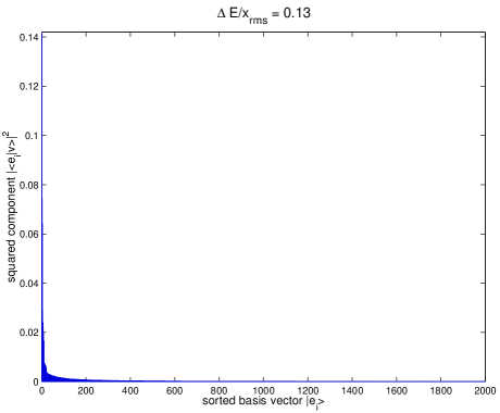
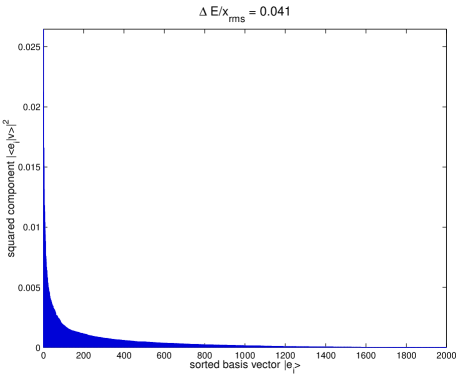
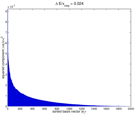
where $j$ and $k$ run from $1$ to $2000$, $x_{jk}$ is a Gaussian random real variable centered at zero with standard deviation $x_{\text{rms}}=0.25$, and $M_{jk}$ is a sparse symmetric matrix consisting of random $0$’s and $1$’s such that the density of $1$’s is $5\%$.  The reason for introducing the $\log(j)$ term in the diagonal is to produce a large variation in the density of states. With this choice the density of states increases exponentially with energy.  Our test matrix is small enough that all eigenvectors can be found without difficulty.  We will consider the distribution of basis components for the eigenvectors of $H$.  In Figure 1 we show the square of the basis components for a given low energy eigenvector $\left|v\right\rangle.$  The basis components are sorted in order of descending importance.  The ratio of $\Delta E$, the average spacing between neighboring energy levels, to $x_{\text{rms}}$ is $0.13$.  We see that the eigenvector is dominated by a few of its most important basis components.  In Figure 2 we show the same plot for another eigenstate but one where the spacing between levels is three times smaller, $\Delta E/x_{\text{rms}}=0.041.$  This eigenvector is not nearly as quasi-sparse.  The effect is even stronger in Figure 3, where we show an eigenvector such that the spacing between levels is $\Delta E/x_{\text{rms}}=0.024$.

Our observations show a strong effect of the density of states on the quasi-sparsity of the eigenvectors.  States with a smaller spacing between neighboring levels tend to have basis components that extend throughout the entire space, while states with a larger spacing tend to be quasi-sparse.  The relationship between extended versus localized eigenstates and the density of states has been studied in the context of Anderson localization and metal-insulator transitions [6].  The simplest example is the tight-binding model for a single electron on a one-dimensional lattice with $Z$ sites,

$$H=\sum_{j}d_{j}\left|j\right\rangle\left\langle j\right|+\sum_{\left\langle jj^{\prime}\right\rangle}t_{jj^{\prime}}\left|j\right\rangle\left\langle j^{\prime}\right|.$$ (8)

$\left|j\right\rangle$ denotes the atomic orbital state at site $j,$ $d_{j}$ is the on-site potential, and $t_{jj^{\prime}}$ is the hopping term between nearest neighbor sites $j$ and $j^{\prime}$.  If both terms are uniform ($d_{j}=d,$ $t_{jj^{\prime}}=t$) then the eigenvalues and eigenvectors of $H$ are

$$Hv_{n} =(d+2t\cos\tfrac{2\pi n}{Z})v_{n},$$ (9)

$$v_{n} =\tfrac{1}{\sqrt{Z}}\sum_{j}e^{i\tfrac{2\pi nj}{Z}}\left|j\right\rangle,$$ (10)

where $n=1,\cdots,Z$ labels the eigenvectors.  In the absence of diagonal and off-diagonal disorder, the eigenstates of $H$ extend throughout the entire lattice.  The eigenvalues are also approximately degenerate, all lying within an interval of size 4$t$.  However, if diagonal and/or off-diagonal disorder is introduced, the eigenvalue spectrum becomes less degenerate.  If the disorder is sufficiently large, the eigenstates become localized to only a few neighboring lattice sites giving rise to a transition of the material from metal to insulator.

We can regard a sparse quantum Hamiltonian as a similar type of system, one with both diagonal and general off-diagonal disorder.  If the disorder is sufficient such that the eigenvalues become non-degenerate, then the eigenvectors will be quasi-sparse.  We reiterate that the most reliable way to determine if the low energy states are quasi-sparse is to use the QSE algorithm.  Intuitively, though, we expect the eigenstates to be quasi-sparse with respect to a chosen basis if the spacing between energy levels is not too small compared with the size of the off-diagonal entries of the Hamiltonian matrix.

4 Finite matrix examples

As a first test of the QSE method, we will find the lowest four energy states of the random symmetric matrix $H$ defined in (7).  So that there is no misunderstanding, we should repeat that diagonalizing a $2000\times 2000$ matrix is not difficult.  The purpose of this test is to analyze the performance of the method in a controlled environment.  One interesting twist is that the algorithm uses only small pieces of the matrix and operates under the assumption that the space may be infinite dimensional.  A sample MATLAB program similar to the one used here has been printed out as a tutorial example in [9].

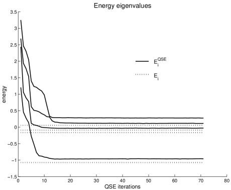
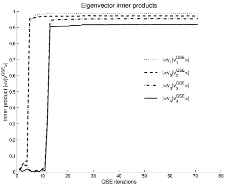
The program starts from a random configuration, 70 basis states for each of the four eigenvectors.  With each iteration we select $10$ replacement basis states for each of the eigenvectors.  In Figure 4 we show the exact energies and the results of the QSE method as functions of iteration number.  In Figure 5 we show the inner products of the normalized QSE eigenvectors with the normalized exact eigenvectors.  We note that all of the eigenvectors were found after about 15 iterations and remained stable throughout successive iterations.  Errors are at the $5$ to $10\%$ level, which is about the theoretical limit one can achieve using this number of basis states.  The QSE method has little difficulty finding several low lying eigenvectors simultaneously because it uses the distribution of basis components for each of the eigenvectors to determine the update process.  This provides a performance advantage over variational-based techniques such as stochastic diagonalization in finding eigenstates other than the ground state.

As a second test we consider a sparse non-Hermitian matrix with complex eigenvalues.  This type of matrix is not amenable to variational-based methods.  We will find the four eigenstates corresponding with eigenvalues with the lowest real part for the random complex non-Hermitian matrix

$$H_{jk}^{\prime}=(1+i\cdot c_{jk})H_{jk}.$$ (11)

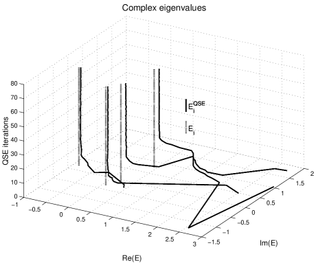
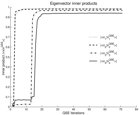
$H_{jk}$ is the same matrix used previously and$\ c_{jk}$ is a uniform random variable distributed between $-1$ and 1.  As before the program is started from a random configuration, 70 basis states for each of the four eigenvectors.  For each iteration $10$ replacement basis vectors are selected for each of the eigenvectors.  In Figure 6 the exact eigenvalues and the results of the QSE run are shown in the complex plane as functions of iteration number.  In Figure 7 we show the inner products of the QSE eigenvectors with the exact eigenvectors.  All of the eigenvectors were found after about 20 iterations and remained stable throughout successive iterations.  Errors were again at about the $5$ to $10\%$ level.

5 $\phi^{4}$ theory in $1+1$ dimensions

We now apply the QSE method to an infinite dimensional quantum Hamiltonian.  We consider $\phi^{4}$ theory in $1+1$ dimensions, a system that is familiar to us from previous studies using Monte Carlo [7] and explicit diagonalization [8].  The Hamiltonian density for $\phi^{4}$ theory in $1+1$ dimensions has the form

$$\mathcal{H}=\tfrac{1}{2}\left(\tfrac{\partial\phi}{\partial t}\right)^{2}+\tfrac{1}{2}\left(\tfrac{\partial\phi}{\partial x}\right)^{2}+\tfrac{\mu^{2}}{2}\phi^{2}+\tfrac{\lambda}{4!}\text{:}\phi^{4}\text{:},$$

where the normal ordering is with respect to the mass $\mu$.  We consider the system in a periodic box of length $2L$.  We then expand in momentum modes and reinterpret the problem as an equivalent Schrödinger equation [7].  The resulting Hamiltonian is

$$H =-\tfrac{1}{2}{\displaystyle\sum_{n}}\tfrac{\partial}{\partial q_{-n}}\tfrac{\partial}{\partial q_{n}}+\tfrac{1}{2}{\displaystyle\sum_{n}}\left(\omega_{n}^{2}(\mu)-\tfrac{\lambda b(\mu)}{8L}\right)\,q_{-n}q_{n}$$ (12)

$$+\tfrac{\lambda}{4!2L}{\displaystyle\sum_{n_{1}+n_{2}+n_{3}+n_{4}=0}}q_{n_{1}}q_{n_{2}}q_{n_{3}}q_{n_{4}}$$

where

$$\omega_{n}(\mu)=\sqrt{\tfrac{n^{2}\pi^{2}}{L^{2}}+\mu^{2}}$$ (13)

and $b(\mu)$ is the coefficient for the mass counterterm

$$b(\mu)={\displaystyle\sum_{n}}\tfrac{1}{2\omega_{n}(\mu)}.$$ (14)

It is convenient to split the Hamiltonian into free and interacting parts with respect to an arbitrary mass $\mu^{\prime}$:

$$H_{free}=-\tfrac{1}{2}{\displaystyle\sum_{n}}\tfrac{\partial}{\partial q_{-n}}\tfrac{\partial}{\partial q_{n}}+\tfrac{1}{2}{\displaystyle\sum_{n}}\omega_{n}^{2}(\mu^{\prime})\,q_{-n}q_{n},$$ (15)

$$H =H_{free}+\tfrac{1}{2}{\displaystyle\sum_{n}}\left(\mu^{2}-\mu^{\prime 2}-\tfrac{\lambda b(\mu)}{8L}\right)q_{-n}q_{n}$$ (16)

$$+\tfrac{\lambda}{4!2L}{\displaystyle\sum_{n_{1}+n_{2}+n_{3}+n_{4}=0}}q_{n_{1}}q_{n_{2}}q_{n_{3}}q_{n_{4}}.$$

$\mu^{\prime}$ is used to define the basis states of our Fock space.  Since $H$ is independent of $\mu^{\prime}$, we perform calculations for different $\mu^{\prime}$ to obtain a reasonable estimate of the error.  It is also useful to find the range of values for $\mu^{\prime}$ which maximizes the quasi-sparsity of the eigenvectors and therefore improves the accuracy of the calculation.  For the calculations presented here, we set the length of the box to size $L=5\pi\mu^{-1}$.  We restrict our attention to momentum modes $q_{n}$ such that $\left|n\right|\leq N_{\max}$, where $N_{\max}=20$.  This corresponds with a momentum cutoff scale of $\Lambda=4\mu.$

To implement the QSE algorithm on this infinite dimensional Hilbert space, we first define ladder operators with respect to $\mu^{\prime}$,

$$a_{n}(\mu^{\prime}) =\tfrac{1}{\sqrt{2\omega_{n}(\mu^{\prime})}}\left[q_{n}\omega_{n}(\mu^{\prime})+\tfrac{\partial}{\partial q_{-n}}\right]$$ (17)

$$a_{n}^{\dagger}(\mu^{\prime}) =\tfrac{1}{\sqrt{2\omega_{n}(\mu^{\prime})}}\left[q_{-n}\omega_{n}(\mu^{\prime})-\tfrac{\partial}{\partial q_{n}}\right].$$ (18)

The Hamiltonian can now be rewritten as

$$H ={\displaystyle\sum_{n}}\omega_{n}(\mu^{\prime})a_{n}^{\dagger}a_{n}+\tfrac{1}{4}(\mu^{2}-\mu^{\prime 2}-\tfrac{\lambda b}{8L}){\displaystyle\sum_{n}}\tfrac{\left(a_{-n}+a_{n}^{\dagger}\right)\left(a_{n}+a_{-n}^{\dagger}\right)}{\omega_{n}(\mu^{\prime})}$$ (19)

$$+\tfrac{\lambda}{192L}{\displaystyle\sum_{n_{1}+n_{2}+n_{3}+n_{4}=0}}\left[\tfrac{\left(a_{n_{1}}+a_{-n_{1}}^{\dagger}\right)}{\sqrt{\omega_{n_{1}}(\mu^{\prime})}}\tfrac{\left(a_{n_{2}}+a_{-n_{2}}^{\dagger}\right)}{\sqrt{\omega_{n_{2}}(\mu^{\prime})}}\tfrac{\left(a_{n_{3}}+a_{-n_{3}}^{\dagger}\right)}{\sqrt{\omega_{n_{3}}(\mu^{\prime})}}\tfrac{\left(a_{n_{4}}+a_{-n_{4}}^{\dagger}\right)}{\sqrt{\omega_{n_{4}}(\mu^{\prime})}}\right].$$

In (19) we have omitted constants contributing only to the vacuum energy.  We represent any momentum-space Fock state as a string of occupation numbers, $\left|o_{-N_{\max}},\cdots,o_{N_{\max}}\right\rangle$, where

$$a_{n}^{\dagger}a_{n}\left|o_{-N_{\max}},\cdots,o_{N_{\max}}\right\rangle=o_{n}\left|o_{-N_{\max}},\cdots,o_{N_{\max}}\right\rangle.$$ (20)

From the usual ladder operator relations, it is straightforward to calculate the matrix element of $H$ between two arbitrary Fock states.

Aside from calculating matrix elements, the only other fundamental operation needed for the QSE algorithm is the generation of new basis vectors.  The new states should be connected to some old basis vector through non-vanishing matrix elements of $H$.  Let us refer to the old basis vector as $\left|e\right\rangle$.  For this example there are two types of terms in our interaction Hamiltonian, a quartic interaction

$${\displaystyle\sum_{n_{1},n_{2},n_{3}}}\left(a_{n_{1}}+a_{-n_{1}}^{\dagger}\right)\left(a_{n_{2}}+a_{-n_{2}}^{\dagger}\right)\left(a_{n_{3}}+a_{-n_{3}}^{\dagger}\right)\left(a_{-n_{1}-n_{2}-n_{3}}+a_{n_{1}+n_{2}+n_{3}}^{\dagger}\right),$$ (21)

and a quadratic interaction

$${\displaystyle\sum_{n}}\left(a_{-n}+a_{n}^{\dagger}\right)\left(a_{n}+a_{-n}^{\dagger}\right).$$ (22)

To produce a new vector from $\left|e\right\rangle$ we simply choose one of the possible operator monomials

$$a_{n_{1}}a_{n_{2}}a_{n_{3}}a_{-n_{1}-n_{2}-n_{3}},\,a_{-n_{1}}^{\dagger}a_{n_{2}}a_{n_{3}}a_{-n_{1}-n_{2}-n_{3}},\cdots,$$ (23)

$$a_{-n}a_{n},\,a_{n}^{\dagger}a_{-n}^{\dagger},\cdots$$

and act on $\left|e\right\rangle$.  Our experience is that the interactions involving the small momentum modes are generally more important than those for the large momentum modes, a signal that the ultraviolet divergences have been properly renormalized.  For this reason it is best to arrange the selection probabilities such that the smaller values of $\left|n_{1}\right|$, $\left|n_{2}\right|$, $\left|n_{3}\right|$ and $\left|n\right|$ are chosen more often.

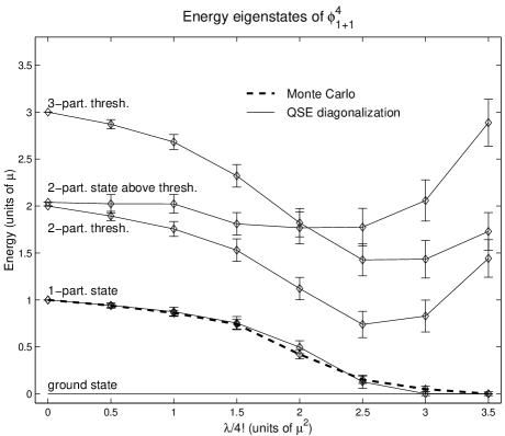
For each QSE iteration, $50$ new basis vectors were selected for each eigenstate and $250$ basis vectors were retained.  The results for the lowest energy eigenvalues are shown in Figure 8.  The error bars were estimated by repeating the calculation for different values of the auxiliary mass parameter $\mu^{\prime}$.

From prior Monte Carlo calculations we know that the theory has a phase transition at $\frac{\lambda}{4!}\approx 2.5\mu^{2}$ corresponding with spontaneous breaking of the $\phi\rightarrow-\phi$ reflection symmetry.  In the broken phase there are two degenerate ground states and we refer to these as the even and odd vacuum states.  In Figure 8 we see signs of a second order phase transition near $\frac{\lambda}{4!}\approx 2.5\mu^{2}$.  Since we are working in a finite volume the spectrum is discrete, and we can track the energy eigenvalues as functions of the coupling.  Crossing the phase boundary, we see that the vacuum in the symmetric phase becomes the even vacuum in the broken phase while the one-particle state in the symmetric phase becomes the odd vacuum.  The energy difference between the states is also in agreement with a Monte Carlo calculation of the same quantities.  The state marking the two-particle threshold in the symmetric phase becomes the one-particle state above the odd vacuum, while the state at the three-particle threshold becomes the one-particle state above the even vacuum.  These one-particle states should be degenerate in the infinite volume limit.  One rather unusual feature is the behavior of the first two-particle state above threshold in the symmetric phase.  In the symmetric phase this state lies close to the two-particle threshold.  But as we cross the phase boundary the state which was the two-particle threshold is changed into a one-particle state.  Thus our two-particle state is pushed up even further to become a two-particle state above the even vacuum and we see a pronounced level crossing.

We note that while the one-particle mass vanishes near the critical point, the energies of the two-particle and three-particle thresholds reach a minimum but do not come as close to zero energy.  It is known that this model is repulsive in the two-particle scattering channel.  In a large but finite volume the ground state and one-particle states do not feel significant finite volume effects.  The two-particle state at threshold, however, requires that the two asymptotic particles be widely separated.  In our periodic box of length 2$L$ the maximal separation distance is $L$ and we expect an increase in energy with respect to twice the one-particle mass of size $\sim V(L)$, where $V$ is the potential energy between particles.  Likewise a three-particle state will increase in energy an amount $\sim 3V(2L/3)$.  Our results indicate that finite volume effects for the excited states are significant for this value of $L$.

6 Summary

We have proposed a new approach which combines both diagonalization and Monte Carlo within a computational scheme.  The motivation for our approach is to take advantage of the strengths of the two computational methods in their respective domains. We remedy sign and phase oscillation problems by handling the interactions of the most important basis states exactly using diagonalization, and we deal with storage and CPU problems by stochastically sampling the contribution of the remaining states.  We discussed the diagonalization part of the method in this paper.  The goal of diagonalization within our scheme is to find the most important basis vectors of the low energy eigenstates and treat the interactions among them exactly.  We have introduced a new diagonalization method called quasi-sparse eigenvector diagonalization which achieves this goal efficiently and can operate using any basis, either orthogonal or non-orthogonal, and any sparse Hamiltonian, either real, complex, Hermitian, non-Hermitian, finite-dimensional, or infinite-dimensional.  Quasi-sparse eigenvector diagonalization is the only method we know which can address all of these problems.

We considered three examples which tested the performance of the algorithm.  We found the lowest energy eigenstates for a random sparse real symmetric matrix, the lowest eigenstates (sorted according to the real part of the eigenvalue) for a random sparse complex non-Hermitian matrix, and the lowest energy eigenstates for an infinite-dimensional Hamiltonian defined by $1+1$ dimensional $\phi^{4}$ theory in a periodic box.

We regard QSE diagonalization as only a starting point for the Monte Carlo part of the calculation.  Once the most important basis vectors are found and their interactions treated exactly, a technique called stochastic error correction is used to sample the contribution of the remaining basis vectors.  This method is introduced in [1].

Acknowledgments

We thank P. van Baal, H. S. Seung, H. Sompolinsky, and M. Windoloski for useful discussions.  Support provided by the National Science Foundation.

Figure 1: Distribution of basis components for an eigenvector where the spacing between consecutive levels is $\Delta E=0.13x_{\text{rms}}$.

Figure 2: Distribution of basis components for an eigenvector where $\Delta E=0.041x_{\text{rms}}$.

Figure 3: Distribution of basis components for an eigenvector where $\Delta E=0.024x_{\text{rms}}$.

Figure 4: Comparison of the four lowest exact energies $E_{i}$ and QSE results $E_{i}^{\text{QSE}}$ as functions of iteration number.

Figure 5: Inner products between the normalized exact eigenvectors $\left|v_{i}\right\rangle$ and the QSE results $\left|v_{i}^{\text{QSE}}\right\rangle$ as functions of iteration number.

Figure 6: Comparison of the four lowest exact eigenvalues $E_{i}$ (sorted by real part) and QSE results $E_{i}^{\text{QSE}}$ in the complex plane as functions of iteration number.

Figure 7: Inner products between the normalized exact eigenvectors $\left|v_{i}\right\rangle$ and the QSE results $\left|v_{i}^{\text{QSE}}\right\rangle$ as functions of iteration number.

Figure 8: Energy eigenvalues of $\phi_{1+1}^{4}$ as functions of the coupling constant.

References

- [1] D. Lee, N. Salwen, M. Windoloski, hep-lat/0010039.
- [2] R. Perry, A. Harindranath, K. Wilson, Phys. Rev. Lett. 24 (1990) 2959; I. Tamm, J. Phys. (USSR) 9 (1945) 449; S. M. Dancoff, Phys. Rev. 78 (1950) 382.
- [3] K. Wilson, Phys. Rev. 140 (1965) B445; S. Glazek, K. Wilson, Phys. Rev. D48 (1993) 5863; S. Glazek, K. Wilson, Phys. Rev. D49 (1994) 4214.
- [4] S. White, Phys. Rev. Lett. 69 (1992) 2863; S. White, Phys. Rev. B48 (1993) 10345.
- [5] T. Husslein, W. Fettes, I. Morgenstern, Int. J. Mod. Phys. C8 (1997) 397; H. de Raedt, M. Frick, Comp. Phys. Rep. 7 (1992) 1.
- [6] P. Biswas, P. Cain, R. Römer, M. Schreiber, cond-mat/0001315; C. Soukoulis, I. Weman, G. Grest, E. Economou, Phys. Rev. B26 (1982) 1838; T. Ziman, Phys. Rev. B26 (1982) 7066; M. Inui, S. Trugman, E. Abrahams, Phys. Rev. B49 (1994) 3190.
- [7] P. Marrero, E. Roura, D. Lee, Phys. Lett. B471 (1999) 45.
- [8] N. Salwen, D. Lee, Phys. Rev. D62 (2000) 025006.
- [9] D. Lee, hep-th/0007010.