Abstract

We show that in the presence of massive particles such as nucleons, the standard low energy expansion in powers of meson momenta and light quark masses in general only converges in part of the low energy region. The expansion of the scalar form factor $\sigma(t)$, for instance, breaks down in the vicinity of $t=4M_{\pi}^{2}$. In the language of heavy baryon chiral perturbation theory, the proper behaviour in the threshold region only results if the multiple internal line insertions generated by relativistic kinematics are summed up to all orders. We propose a method that yields a coherent representation throughout the low energy region while keeping Lorentz and chiral invariance explicit at all stages. The method is illustrated with a calculation of the nucleon mass and of the scalar form factor to order $p^{4}$.

                        Contents

1	Introduction	1
2	Effective Lagrangian	2
3	Scalar form factor	3
4	Low energy expansion near threshold	4
5	Infrared singularities in the self energy	5
	Singular and regular parts	5
	Properties of the decomposition	5
	Representation in terms of modified propagators	5
	Dispersive representation	5
6	Generalization	6
	Singular and regular parts	6
	Uniqueness of the decomposition	6
7	Comparison with HB $\chi$PT	7
	Lorentz invariance	7
	Chiral symmetry	7
	Infrared part as an alternative regularization	7
8	Renormalization	8
	Self energy	8
	Renormalization scale	8
	Other one loop graphs	8
9	Convergence of the chiral expansion, explicit representations	9
	Explicit representation of the self energy	9
	Chiral expansion of the self energy	9
	Other one loop integrals	9
10	Chiral expansion of the nucleon mass	10
11	Wave function renormalization	11
12	Scalar form factor to order $p^{4}$	12
	Evaluation of the graphs	12
	Result	12
	Unitarity	12
	Value at the Cheng-Dashen point	12
	The $\sigma$-term	12
13	Discussion	13
	Reordering of the perturbation series	13
	The role of the $\Delta(1232)$	13
	Comparison with the static model	13
	Momentum space cutoff	13
14	Conclusion	14
A	Low energy representation for the triangle graph	A
B	Infrared parts of some loop integrals	B
C	$\pi N$ scattering in tree approximation	C
D	Contributions generated by the $\Delta$	D

1 Introduction

The effective low energy theory of the strong interaction is based on a simultaneous expansion of the Green functions of QCD in powers of the external momenta and of the quark masses (“chiral expansion”). In the vacuum sector, where the only low energy singularities are those generated by the Goldstone bosons, dimensional regularization yields homogeneous functions of the momenta and Goldstone masses, so that each graph has an unambiguous order in the chiral expansion. In the sector with baryon number 1, however, the low energy structure is more complicated. The corresponding effective theory can be formulated in manifestly Lorentz invariant form [1], but it is not a trivial matter to keep track of the chiral order of graphs containing loops within that framework: The chiral expansion of the loop graphs in general starts at the same order as the corresponding tree graphs, so that the renormalization of the divergences requires a tuning also of those effective coupling constants that occur at lower order – in particular, the nucleon mass requires renormalization at every order of the series.

Most of the recent calculations avoid this complication with a method referred to as heavy baryon chiral perturbation theory (HB $\chi$PT) [2, 3, 4, 5]. The starting point of that method is the same Lorentz invariant effective Lagrangian that occurs in the relativistic approach. The loop graphs, however, are evaluated differently: The Dirac-spinor that describes the nucleon degrees of freedom is reduced to a two-component field and the baryon kinematics is expanded around the nonrelativistic limit. At the end of the calculation, the amplitude may then be recast into Lorentz invariant form. This method keeps track of the chiral power counting at every step of the calculation, at the price of manifest Lorentz invariance.

Mojžiš [6] and Fettes et al. [7] have evaluated the $\pi N$ scattering amplitude to order $p^{3}$ within that framework. The explicit result is remarkably simple, the one loop graphs being expressible in terms of elementary functions. On general grounds, the outcome of this calculation must be the same as what is obtained if the representation of the scattering amplitude given in [1] is expanded around the nonrelativistic limit – that representation also holds to order $p^{3}$. Indeed, Ellis and Tang [8] have shown that this is the case.

Quite apart from the fact that the nonrelativistic expansion turns the effective Lagrangian into a rather voluminous object and that care is required to properly analyze the corresponding loop graphs, HB $\chi$PT suffers from a deficiency: The corresponding perturbation series fails to converge in part of the low energy region. The problem is generated by a set of higher order graphs involving insertions in nucleon lines. A similar phenomenon also appears in the effective field theory of the $NN$-interaction [13]. It arises from the nonrelativistic expansion and does not occur in the relativistic formulation of the effective theory.

The purpose of the present paper is to present a method that exploits the advantages of the two techniques and avoids their disadvantages. In sections 3 and 4, we demonstrate the need to sum up certain graphs of HB $\chi$PT, using the example of the scalar nucleon form factor. Next, we show that the infrared singularities of the various one loop graphs occurring in the chiral perturbation series can be extracted in a relativistically invariant fashion (sections 5 and 6). The method we are using here follows the approach of Tang and Ellis [8]. There is a slight difference, insofar as we do not rely on the chiral expansion of the loop integrals – that expansion does not always converge. A comparison with HB $\chi$PT is given in section 7, where we also show that our procedure may be viewed as a novel method of regularization, which we call “infrared regularization”. The method represents a variant of dimensional regularization. While that scheme permits a straightforward counting of the powers of momentum at high energies, infrared regularization preserves the low energy power counting rules that underly chiral perturbation theory. Renormalization is discussed in section 8. We then analyze the convergence of the chiral expansion of the one loop integrals and show that the expansion coefficients relevant for $\pi N$ scattering can be expressed in terms of elementary functions (section 9). Whenever that expansion converges, the result agrees with the one obtained within HB $\chi$PT. We also construct an explicit low energy representation of the triangle graph, for which the nonrelativistic expansion fails. The method is illustrated with an evaluation of the chiral perturbation series for the nucleon mass, the wave function renormalization constant and the scalar form factor. The physics of the result obtained for the form factor and for the $\sigma$-term is discussed in sections 12 and 13. We demonstrate that a significant part of those infrared singularities that are proportional to $M_{\pi}^{3}$ is common to the form factor and to the $\pi N$ scattering amplitude and thus drops out when considering the predictions of the theory. The observation leads to a specific reordering of the chiral perturbation series that reduces the matrix elements of the perturbation quite substantially. The effects generated by the $\Delta(1232)$ are discussed in some detail (appendix D) and we also compare our framework with the ancestor of the effective theory described here: the static model. Section 14 contains our conclusions.

2 Effective Lagrangian

The variables of the effective theory are the meson field $U(x)\in\mbox{SU(2)}$ and the Dirac spinor $\psi(x)$ describing the degrees of freedom of the nucleon. The effective Lagrangian contains two pieces,

$${\cal L}_{eff}={\cal L}_{\pi}+{\cal L}_{N}\;.$$

The first part is the well-known meson Lagrangian, which only involves the field $U(x)$ and an even number of derivatives thereof. For the second part, which is bilinear in $\bar{\psi}(x)$ and $\psi(x)$, the derivative expansion contains odd as well as even terms:

$${\cal L}_{N}={\cal L}_{N}^{(1)}+{\cal L}_{N}^{(2)}+{\cal L}_{N}^{(3)}+\ldots$$

The explicit expressions involve the quantities $u$, $u_{\mu}$, $\Gamma_{\mu}$ and $\chi_{\pm}$. In the absence of external vector and axial fields, these are given by

$$u^{2}\! \!=\! \!U\;,\hskip 15.00002ptu_{\mu}=iu^{\dagger}\partial_{\mu}Uu^{\dagger}\;,\hskip 15.00002pt\Gamma_{\mu}=\mbox{$\frac{1}{2}$}[u^{\dagger},\partial_{\mu}u]\;,\hskip 15.00002pt\chi_{\pm}=u^{\dagger}\chi u^{\dagger}\pm u\chi^{\dagger}u\;.$$

At leading order, the effective Lagrangian is fully determined by the nucleon mass and by the matrix element of the axial charge ($m$ and $g_{A}$ denote the corresponding leading order values and $D_{\mu}\equiv\partial_{\mu}+\Gamma_{\mu}$):

$${\cal L}^{(1)}_{N}=\bar{\psi}\left(iD\!\!\!\!/-m\right)\psi+\mbox{$\frac{1}{2}$}\,g_{A}\,\bar{\psi}\,u/\,\gamma_{5}\psi\;,$$

We disregard isospin breaking effects. The Lagrangian of order $p^{2}$ then contains four independent coupling constants

$${\cal L}^{(2)}_{N}\! \!=\! \!c_{1}\,\langle\chi_{+}\rangle\,\bar{\psi}\,\psi-\frac{c_{2}}{4m^{2}}\,\langle u_{\mu}u_{\nu}\rangle\,(\bar{\psi}\,D^{\mu}\!D^{\nu}\!\psi+\mbox{h.c.})\,$$

$$\!+\frac{c_{3}}{2}\,\langle u_{\mu}u^{\mu}\rangle\,\bar{\psi}\,\psi-\frac{c_{4}}{4}\,\bar{\psi}\,\gamma^{\mu}\,\gamma^{\nu}\,[u_{\mu},u_{\nu}]\,\psi\;.$$

Below, we apply the machinery to the scalar form factor. This quantity does not receive any contribution from ${\cal L}^{(3)}_{N}$, but two of the terms in ${\cal L}^{(4)}_{N}$,

$${\cal L}_{N}^{(4)}=-\frac{e_{1}}{16}\langle\chi_{+}\rangle^{2}\bar{\psi}\,\psi+\frac{e_{2}}{4}\,\langle\chi_{+}\rangle\,\raisebox{1.49994pt}{\framebox{\rule[1.49994pt]{0.0pt}{0.0pt}\,}}\,(\bar{\psi}\,\psi)+\ldots\;\;,$$ (2)

do generate contributions proportional to $e_{1}M_{\pi}^{4}$ and $e_{2}M_{\pi}^{2}\,t$, respectively.

3 Scalar form factor

We first wish to show that, in the sector with baryon number 1, the standard chiral expansion in powers of meson momenta and quark masses converges only in part of the low energy region. For definiteness, we consider the scalar form factor of the nucleon in the isospin limit ($m_{u}=m_{d}=\hat{m}$),

$$\langle N(P^{\prime},s^{\prime})|\,\hat{m}\,(\bar{u}u+\bar{d}d)\,|N(P,s)\rangle=\bar{u}^{\prime}u\;\sigma(t),\hskip 20.00003ptt=(P^{\prime}-P)^{2}\;.$$

The first two terms occurring in the low energy expansion of this form factor were worked out long ago, on the basis of a one loop calculation within the Lorentz invariant formulation of the effective theory [1]. In that expansion, $t$, $\hat{m}$ and $M_{\pi}^{2}$ are treated as small quantities of $O(p^{2})$, while the nucleon mass represents a term of $O(p^{0})$. In view of the quark mass factor occurring in the definition of $\sigma(t)$, the low energy expansion starts at order $p^{2}$, with a momentum independent term generated by ${\cal L}_{N}^{(2)}$:

$$\sigma(t)=-4c_{1}\,M_{\pi}^{2}+\frac{3\,g_{A}^{2}M_{\pi}^{2}m_{N}}{4F_{\pi}^{2}}\left\{(t-2M_{\pi}^{2})\,\gamma(t)-\frac{M_{\pi}}{8\pi m_{N}}\right\}+O(p^{4})$$ (3)

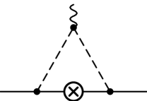
The constant $c_{1}$ occurring here is a renormalized version of the bare coupling constant in eq. (2). Since the renormalization depends on the framework used, we do not discuss it at this preliminary stage. The contribution of order $p^{3}$ is generated by the triangle graph shown in fig. 1 and is fully determined by $F_{\pi}$ and $g_{A}$.

Figure 1: Triangle graph. The solid, dashed and wiggly lines represent nucleons, pions and an external scalar source, respectively.

The term involves the convergent scalar loop integral

$$\gamma(t)=\frac{1}{i}\!\int\!\!\frac{d^{4}k}{(2\pi)^{4}}\frac{1}{(M^{2}\!-k^{2}\!-\!i\epsilon)\,(M^{2}\!-\!(k\!-\!q)^{2}\!-\!i\epsilon)\,(m^{2}\!-\!(P\!-\!k)^{2}\!-\!i\epsilon)}$$ (4)

Here and in the following, we identify the masses occurring in the loop integrals with their leading order values, $M_{\pi}\rightarrow M$, $m_{N}\rightarrow m$.

The function $\gamma(t)$ represents a quantity of $O(1/p)$. Since the external nucleon lines are on the mass shell, it exclusively depends on $t=q^{2},\,M$ and $m$. The function is analytic in $t$ except for a cut along the positive real axis, starting at $t=4\,M^{2}$. The triangle graph also shows up in the analysis of the $\pi N$ scattering amplitude to one loop, so that the function $\gamma(t)$ is relevant also for that case.

The imaginary part of $\gamma(t)$ can be expressed in terms of elementary functions [1]:

$$\mbox{Im}\gamma(t)=\frac{\theta(t-4M^{2})}{8\pi\sqrt{\,t\,(4m^{2}-t)}}\;\arctan\frac{\sqrt{(t-4M^{2})(4m^{2}-t)}}{t-2M^{2}}\;.$$ (5)

Dropping corrections of order $t/m^{2}=O(p^{2})$, this expression simplifies to

$$\mbox{Im}\gamma(t)=\frac{\theta(t-4M^{2})}{16\pi m\sqrt{t}}\left\{\arctan\frac{2m\sqrt{\,t-4M^{2}}}{t-2M^{2}}+O(p^{2})\right\}\;.$$ (6)

The problem addressed above shows up in this formula: The quantity

$$x=\frac{2m\sqrt{\,t-4M^{2}}}{t-2M^{2}}$$

represents a term of $O(1/p)$. The standard chiral expansion of $\mbox{Im}\gamma(t)$ thus corresponds to the series $\arctan x=\frac{1}{2}\,\pi-1/x+\frac{1}{3}\,(1/x)^{3}+\ldots$ This series, however, only converges for $|x|>1$. In the vicinity of $t=4M^{2}$, the condition is not met, so that the chiral expansion diverges. The problem arises because the quantity $x$ takes small values there, while the low energy expansion treats it as a large term of $O(1/p)$. In the region $|x|<1$, we may instead use the convergent series $\arctan x=x-\frac{1}{3}\,x^{3}+\ldots\;$, but this amounts to an expansion in inverse powers of $p$.

The rapid variation of the form factor near $t=4M^{2}$ is related to the fact that the function $\arctan z$ exhibits branch points at $z=\pm\,i$. The analytic continuation of $\gamma(t)$ to the second sheet therefore contains a branch point just below threshold:

$$\frac{(t-4M^{2})(4m^{2}-t)}{(t-2M^{2})^{2}}=-1\hskip 20.00003pt\rightarrow\hskip 20.00003ptt=4M^{2}-\frac{M^{4}}{m^{2}}\;.$$

This implies that, in the threshold region, the form factor does not admit an expansion in powers of meson momenta and quark masses. As was shown in ref. [3], the heavy baryon perturbation series to $O(p^{3})$ coincides with the chiral expansion of the relativistic result [1] and it was noted in ref. [5] that this representation does not make sense near $t=4M^{2}$. The corresponding imaginary part amounts to the approximation $\arctan x\rightarrow\frac{1}{2}\,\pi$, so that the singularity structure on the second sheet is discarded. Within HB $\chi$PT, an infinite series of internal line insertions must be summed up to properly describe the behaviour of the form factor near threshold. The relativistic formula (3), on the other hand, does apply in the entire low energy region, because it involves the full function $\gamma(t)$ rather than the first one or two terms in the chiral expansion thereof.

4 Low energy expansion near threshold

We conclude that in the threshold region, the low energy structure cannot be analyzed in terms of the standard chiral expansion. The first two terms of this expansion, i.e. the first two terms of the heavy baryon perturbation series,

$$\mbox{Im}\gamma_{1}(t)=\frac{\theta(t-4M^{2})}{32\pi mM}\left\{\frac{\pi M}{\sqrt{t}}-\frac{\alpha\,(t-2\,M^{2})}{\sqrt{\,t\,(t-4M^{2})}}\right\}\;,$$ (7)

provide a decent representation only if $t$ is not close to threshold.

To resolve the structure in the threshold region, we need to consider an expansion that does not treat the quantity $x$ as large. This can be done by replacing the variable $t$ with the dimensionless parameter

$$\xi=\frac{\sqrt{\,t-4M^{2}}}{\alpha\,M}\;,\hskip 20.00003pt\alpha=\frac{M}{m}\;,$$

and expanding the amplitude at fixed $\xi$, so that the momentum transfer

$$t=(4+\alpha^{2}\xi^{2})\,M^{2}$$

stays close to threshold.

For the imaginary part, the expansion at fixed $\xi$ takes the form

$$\mbox{Im}\gamma(t)=\frac{\theta(t-4M^{2})}{32\pi mM}\left\{\arctan\xi+O(p^{2})\right\}\;.$$

At large values of $\xi$, this representation smoothly joins the one provided by the heavy baryon expansion, where $t/M^{2}$ is kept fixed. To amalgamate the two, we note that, in the threshold region, the quantity $\mbox{Im}\gamma_{1}(t)$ reduces to the first two terms of the series $\arctan\xi\equiv\frac{1}{2}\,\pi-\arctan 1/\xi=\frac{1}{2}\,\pi-1/\xi+\ldots$ Hence the difference between $\mbox{Im}\gamma(t)$ and the first two terms of the heavy baryon perturbation series is approximately given by

$$\mbox{Im}\gamma_{2}(t)=\frac{\theta(t-4M^{2})}{32\pi mM}\left\{\frac{\alpha\,M}{\sqrt{\,t-4M^{2}}}-\arctan\frac{\alpha\,M}{\sqrt{\,t-4M^{2}}}\right\}\;.$$ (8)

Outside the threshold region, $\mbox{Im}\gamma_{2}(t)$ is negligibly small – in the chiral counting of powers, it represents a term of order $p^{2}$. The representation

$$\mbox{Im}\gamma(t)=\mbox{Im}\gamma_{1}(t)+\mbox{Im}\gamma_{2}(t)+O(p)$$ (9)

holds irrespective of whether $t/M^{2}$ or $\xi$ is held fixed. Indeed, one may verify that on the entire interval $4M^{2}\leq t\leq 20\,M^{2}$, the formula differs from the expression in eq. (6) by less than 1 %.

Finally, we turn to the function $\gamma(t)$ itself. As mentioned above, the loop integral cannot be expressed in terms of elementary functions. We may, however, give an explicit representation that holds to first nonleading order of the low energy expansion, throughout the low energy region. The calculation is described in appendix A. It leads to a representation of the form

$$\gamma(t)=\gamma_{1}(t)+\gamma_{2}(t)+O(p)\;.$$ (10)

The first term corresponds to the result obtained in HB $\chi$PT [3]. This piece explodes in the vicinity of the threshold, like its imaginary part. The explicit expression for the remainder reads

$$\gamma_{2}(t)=\frac{1}{32\pi mM}\left\{\frac{\alpha\,M}{\sqrt{4M^{2}-t}}-\mbox{ln}\left\{1+\frac{\alpha\,M}{\sqrt{4M^{2}-t}}\right\}\right\}\;.$$ (11)

In the language of HB $\chi$PT, this term is generated by multiple internal line insertions. It takes significant values only in the immediate vicinity of threshold, where it cures the deficiencies of $\gamma_{1}(t)$. Indeed, this term does account for the branch cut at $t=4M^{2}-M^{4}/m^{2}$, which is missing in $\gamma_{1}(t)$.

5 Infrared singularities in the self energy

Having established the need to sum certain graphs of the heavy baryon chiral perturbation series to all orders, we now formulate a general method that leads to a representation where the relevant graphs are automatically accounted for. The method relies on dimensional regularization: We analyze the infrared singularities of the loop integrals for an arbitrary value of the dimension $d$.

Figure 2: Self energy

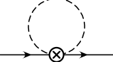
To explain the essence of the method, we first consider the simplest example: the self-energy graph shown in fig. 2. We again focus on the corresponding scalar loop integral

$$H=\frac{1}{i}\int\!\!\frac{d^{d}k}{(2\pi)^{d}}\,\frac{1}{(M^{2}-k^{2}-i\epsilon)\,(m^{2}-(P-k)^{2}-i\epsilon)}\;.$$

5.1 Singular and regular parts

The integral $H=H(P^{2},M^{2},m^{2})$ converges for $d<4$. We need to analyze it for nucleon momenta close to the mass shell: $P=m\,v+r$, where $v$ is a timelike unit vector and $r$ is a small quantity of order $p$. It is convenient to work with the dimensionless variables

$$\Omega=\frac{P^{2}-m^{2}-M^{2}}{2mM}\;,\hskip 20.00003pt\alpha=\frac{M}{m}\;,$$ (12)

which represent quantities of order $\Omega=O(p^{0})$ and $\alpha=O(p)$, respectively (recall that $m$ is the larger one of the two masses, $\alpha\simeq\frac{1}{7}$).

In the limit $M\rightarrow 0$, the integral develops an infrared singularity, generated by small values of the variable of integration, $k=O(p)$. In that region, the first factor in the denominator is of $O(p^{2})$, while the second is of order $p$. Accordingly, the chiral expansion of $H$ contains contributions of $O(p^{\,d-3})$. We may enhance these by considering small dimensions. For $d<3$, the leading term in the chiral expansion of $H$ exclusively stems from the region $k=O(p)$, which generates a singular contribution of order $p^{\,d-3}$, as well as nonleading terms of order $p^{\,d-2}$, $p^{\,d-1}$, $\ldots$ The remainder of the integration region does not contain infrared singularities and thus yields a contribution that can be expanded in an ordinary power series. For sufficiently large, negative values of $d$, the infrared region dominates the chiral expansion to any desired order.

To work out the infrared singular piece, we use the standard Schwinger-Feynman-parametrization

$$\frac{1}{a\,b}=\int_{0}^{1}\!\frac{dz}{\{\,(1-z)\,a+z\,b\,\}^{2}}\;.$$ (13)

Performing the integration over $k$, we obtain

$$H\! \!=\! \!\kappa\!\int_{0}^{1}\!\!dz\,C^{\,\frac{d}{2}-2}\;,\hskip 20.00003pt\kappa=(4\pi)^{-\frac{d}{2}}\,\,m^{\,d-4}\,\Gamma(2-\mbox{$\frac{d}{2}$})\;,$$ (14)

$$C\! \!=\! \!z^{2}-2\,\alpha\,\Omega\,z\,(1-z)+\alpha^{2}(1-z)^{2}-i\epsilon\;.$$

In this representation, the infrared singularity arises from small values of $z$: There, the factor $C$ vanishes if $\alpha$ tends to zero. We may isolate the divergent part by scaling the variable of integration, $z=\alpha\,u$. The upper limit then becomes large. We extend the integration to $\infty$ and define the infrared singular part of the loop integral by

$$I\! \!=\! \!\kappa\!\int_{0}^{\infty}\!\!dz\,C^{\,\frac{d}{2}-2}=\kappa\,\alpha^{d-3}\!\!\int_{0}^{\infty}\!\!du\,D^{\,\frac{d}{2}-2}\;,$$ (15)

$$D\! \!=\! \!1-2\,\Omega\,u+u^{2}+2\,\alpha\,u\,(\Omega\,u-1)+\alpha^{2}\,u^{2}-i\epsilon\;.$$

For short, we also refer to $I$ as the infrared part of $H$. The remainder is given by

$$R=-\kappa\int_{1}^{\infty}\!\!dz\,C^{\,\frac{d}{2}-2}\;.$$ (16)

The decomposition

$$H=I+R$$ (17)

neatly separates the infrared singular part from the regular part: For noninteger values of the dimension, the chiral expansion of $I$ exclusively contains fractional powers of $p$,

$$I=O(p^{\,d-3})+O(p^{\,d-2})+O(p^{\,d-1})+\ldots\;,$$

while the corresponding expansion of $R$ is an ordinary Taylor series,

$$R=O(p^{\,0})+O(p^{\,1})+O(p^{\,2})+\ldots$$

5.2 Properties of the decomposition

For an arbitrary value of $d$, the explicit expressions for the quantities $H$, $I$, $R$ involve hypergeometric functions. In four dimensions, the corresponding integrals are elementary. We will give the explicit representations for $d=4$ when we discuss renormalization (see sections 8 and 9).

In terms of the dimensionless variables $\alpha$ and $\Omega$, the chiral expansion of the infrared part takes the form

$$I=m^{d-4}\alpha^{d-3}\left(\rule{0.0pt}{10.00002pt}\,i\rule{0.50003pt}{0.0pt}^{0}+\alpha\,i\rule{0.50003pt}{0.0pt}^{1}+\alpha^{2}\,i\rule{0.50003pt}{0.0pt}^{2}+\ldots\;\right)\;.$$ (18)

The coefficients $i\rule{0.50003pt}{0.0pt}^{n}$, which only depend on $\Omega$, are obtained by expanding the integrand in eq. (15) in powers of $\alpha$. The corresponding explicit expressions also involve hypergeometric functions. The expansion coefficients of the remainder, on the other hand, are simple polynomials of $\Omega$:

$$R=\frac{m^{d-4}\,\Gamma(2-\frac{d}{2})}{(4\pi)^{\frac{d}{2}}\,(d-3)}\left\{1-\alpha\,\Omega+\alpha^{2}\,\frac{1+(d-6)\,\Omega^{2}}{(d-5)}+\ldots\right\}\;.$$ (19)

The series contains poles at $d=3,\,4,\,5\ldots\,$ We now wish to show that, for $d<3$, the chiral expansion of $R$ converges throughout the low energy region.

The integrand of the representation (16) is analytic in $\alpha$, except for the cuts associated with the zeros of $C$. These are located at

$$\alpha=\frac{z}{z-1}\,\left(-\Omega\pm\sqrt{\Omega^{2}-1}\right)\;.$$

The expansion of the integrand thus converges in the disk

$$|\alpha|<|\,\Omega\pm\sqrt{\Omega^{2}-1}\,|\;.$$ (20)

The condition is obeyed for all real values of $\Omega$ in the interval

$$-\frac{1+\alpha^{2}}{2\,\alpha}<\Omega<\frac{1+\alpha^{2}}{2\,\alpha}\;.$$

This range corresponds to $0\!<P^{2}\!<2m^{2}+2M^{2}$ and thus generously covers the entire low energy region. Moreover, for $d<3$, the integral converges uniformly, so that $R$ is analytic in $\alpha$: The series (19) converges for all values of $\Omega$ in the above interval.

In the case of $I$, the representation (15) is relevant. The zeros of the term $D$ are located at

$$\alpha=\frac{1}{u}-\Omega\pm\sqrt{\Omega^{2}-1}\;.$$

In the range $-1<\Omega<1$, the square root is imaginary, so that the zeros occur at $|\alpha|^{2}=(1/u-\Omega)^{2}+1-\Omega^{2}$. This expression has a minimum at $u=1/\Omega$. On the entire interval of integration, the chiral expansion of the integrand thus converges if $|\alpha|^{2}<1-\Omega^{2}$, or, equivalently

$$-\sqrt{1-\alpha^{2}}<\Omega<\sqrt{1-\alpha^{2}}\;.$$ (21)

Again, the integral converges uniformly for $d<3$. Hence the series (18) converges if $\Omega$ is in the range (21). This interval is considerably more narrow than the one found above, but in the present context, the above result suffices: It demonstrates that the two parts occurring in the decomposition of the self energy can unambiguously be characterized by their analytic properties at low energies. Since the functions $I$, $R$ are analytic in the external momenta, their values are uniquely determined also outside the above region. Indeed, we will show in section 9 that the chiral expansion of $I$ also converges in the entire low energy region.

5.3 Representation in terms of modified propagators

It is instructive to interpret the above decomposition in terms of the formula (13). The infrared part results if the integral is taken from $0$ to $\infty$ rather than from $0$ to $1$,

$$\int_{0}^{\infty}\!\frac{dz}{\{\,(1-z)\,a+z\,b\,\}^{2}}=\frac{1}{a\,(b-a)}\;.$$

This shows that the decomposition (17) corresponds to the two terms in the algebraic identity

$$\frac{1}{a\,b}=\frac{1}{a\,(b-a)}-\frac{1}{b\,(b-a)}\;.$$ (22)

Note, however, that the $i\epsilon$-prescription drops out in the difference $b-a$, so that the integral over $k$ of the individual terms on the right is ambiguous. To avoid the ambiguity, we may for instance equip the two masses with different imaginary parts. The proper expression for the infrared part reads

$$I=\frac{1}{i}\int\!\!\frac{d^{d}k}{(2\pi)^{d}}\,\frac{1}{(M^{2}-k^{2}-i\epsilon)\,(m^{2}-P^{2}+2Pk-M^{2}-i\epsilon)}\;.$$ (23)

It differs from $H$ in that the term $k^{2}$ occurring in the nucleon propagator is replaced by $M^{2}$. The regular part, on the other hand, is given by

$$R=-\frac{1}{i}\int\!\!\frac{d^{d}k}{(2\pi)^{d}}\,\frac{1}{(m^{2}-(P-k)^{2}-i\epsilon)\,(m^{2}-P^{2}+2Pk-M^{2}-i\epsilon)}\;.$$ (24)

The expression involves two heavy particle propagators, one where the term with $k^{2}$ is retained, one where this term is replaced by $M^{2}$.

The function $H$ is symmetric with respect to an interchange of $M$ and $m$. The term $I$ collects those contributions of the expansion in powers of $\alpha=M/m$ that involve fractional powers of $M$, while $R$ collects the fractional powers of $m$. The operation $M\leftrightarrow m$, $k\leftrightarrow P-k$ interchanges $a$ and $b$, so that the two terms on the r.h.s. of eq. (22) are mapped into one another. This suggests that an interchange of the two masses takes $I$ into $R$ and vice versa. The argument does not go through, however: The difference in the $i\epsilon$-prescriptions shows that the operation does not take the integral in eq. (23) into the one in eq. (24). The sum $I+R$, of course, is symmetric under an interchange of the two masses.

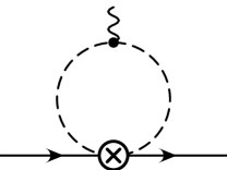
In the heavy baryon chiral perturbation series, the scalar self energy graph of fig. 2 is replaced by an infinite string of one loop graphs,

Figure 3: Internal line insertions. The double line denotes the heavy baryon propagator $[2m\,v\cdot(k-r)-i\epsilon]^{-1}$, the cross an insertion of $(k-r)^{2}$.

involving an arbitrary number of internal line insertions (fig. 3). The corresponding scalar loop integrals are obtained from the relativistic version with $P=m\,v+r$, treating both $r$ and $k$ as small quantities of order $p$ and expanding the nucleon propagator in powers of $p$:

$$\frac{1}{2m\,v\cdot(k-r)-(k-r)^{2}-i\epsilon}\! \!=\!$$

$$\!\frac{1}{2m\,v\cdot(k-r)-i\epsilon}+\frac{(k-r)^{2}}{\{2m\,v\cdot(k-r)-i\epsilon\}^{2}}+\ldots$$

The integral over the leading term converges for $d<3$, yielding a contribution of order $p^{\,d-3}$ that depends on the vector $r$ only through the projection $v\cdot r$. The integral over the second term of the series converges for $d<2$ and yields a term of order $p^{\,d-2}$, etc. The individual contributions are not Lorentz invariant, but the series may be reordered in such a manner that only the Lorentz invariant combination $2m\,v\cdot r+r^{2}=P^{2}-m^{2}$ enters: The heavy baryon series then reproduces the expansion of $I$ in eq. (18), term by term.

To demonstrate that this is so, we recall that the infrared part dominates the chiral expansion to any desired order if $d$ is taken sufficiently negative: For $d<3-n$, the region $k=O(p)$ yields all of the terms in the chiral expansion of the integral $H$, up to and including $p^{\,d-3+n}$. In that region of integration, however, it is legitimate to interchange the integration with the expansion. This is precisely what is done in the heavy baryon approach. Hence that approach does yield the expansion of $I$, to any finite order: The infrared part of the relativistic loop integral represents the sum of the corresponding integrals occurring in the heavy baryon series. The difference between the two formulations of the effective theory resides in the regular part: In the heavy baryon approach, this part is absent. The representation (24) shows that $R$ corresponds to a loop formed with two nucleon lines – evaluating integrals of this type in the manner described above, the rules of HB $\chi$PT [15] indeed yield $R=0$, order by order.

5.4 Dispersive representation

The function $H(P^{2},M^{2},m^{2})$ obeys a dispersion relation, which in four dimensions requires one subtraction. Setting $s=P^{2}$ and suppressing the other variables, the relation takes the form

$$H(s)\! \!=\! \!H(s_{0})+\frac{s-s_{0}}{\pi}\!\int_{s_{+}}^{\infty}\frac{ds^{\prime}}{(s^{\prime}-s_{0})\,(s^{\prime}-s-i\epsilon)}\;\mbox{Im}\,H(s^{\prime})\;,$$ (25)

$$\mbox{Im}\,H(s)\! \!=\! \!\frac{\;\rho(s)}{16\,\pi\,s}\;\theta(s-s_{+})\;,\hskip 20.00003pts_{\pm}=(m\pm M)^{2}\;.$$

The function $\rho(s)$ stands for the familiar two-body phase space factor

$$\rho(s)=\sqrt{(s-s_{+})\,(s-s_{-})}=2\,Mm\sqrt{\Omega^{2}-1}\;.$$

The logarithmic divergence of the loop integral manifests itself in the subtraction constant $H(s_{0})$, which contains a pole at $d=4$. If we subtract at threshold, $s_{0}=s_{+}$, the subtraction constant is given by

$$H(s_{+})=\frac{\Gamma(2-\frac{d}{2})}{(4\pi)^{\frac{d}{2}}(d-3)}\;\frac{m^{d-3}+M^{d-3}}{(m+M)}\;.$$

The structure of this expression is typical: It contains a term with a fractional power of $M$ and one with a fractional power of $m$, representing the infrared singular and regular parts, respectively,

$$I(s_{+})\! \!=\! \!\frac{\Gamma(2-\frac{d}{2})}{(4\pi)^{\frac{d}{2}}(d-3)}\;\frac{M^{d-3}}{(m+M)}\;,$$

$$R(s_{+})\! \!=\! \!\frac{\Gamma(2-\frac{d}{2})}{(4\pi)^{\frac{d}{2}}(d-3)}\;\frac{m^{d-3}}{(m+M)}\;.$$

The dispersion relation (25) is a variant of the formula (14): In the limit $d\rightarrow 4$, the corresponding representation for $H(s)-H(s_{+})$ is proportional to $\int_{0}^{1}dz\,\mbox{ln}(C/C_{+})$, where $C_{+}$ is the value of $C$ at $s=s_{+}$. Since $C$ is linear in $s$,

$$C\! \!=\! \!\frac{z(1-z)}{m^{2}}\;(s^{\prime}-s-i\epsilon)\;,$$

$$s^{\prime}\! \!=\! \!\frac{m^{2}}{1-z}+\frac{M^{2}}{z}\;,\hskip 20.00003pt\frac{ds^{\prime}}{\rho(s^{\prime})}=\frac{|dz|}{|z(1-z)|}\;,$$

the argument of the logarithm reduces to $(s^{\prime}-s-i\epsilon)/(s^{\prime}-s_{+})$. With an integration by parts this indeed leads to eq. (25). Note that, on the interval $0<z<1$, the function $s^{\prime}=s^{\prime}(z)$ has a minimum at

$$z_{min}=\frac{M}{m+M}\;,\hskip 20.00003pts^{\prime}_{min}=s_{+}\;.$$

The map $z\rightarrow s^{\prime}$ thus covers the interval $(m+M)^{2}<s^{\prime}<\infty$ twice.

In the Feynman parameter representation, the only difference between $H$, $I$ and $R$ is that the integrations extend over different intervals. The one relevant for $R$ is $1<z<\infty$, which is mapped onto $-\infty<s^{\prime}<0$. Accordingly, $R$ has a cut along the negative real axis, but is analytic in the right half plane. The discontinuity across the cut is only half as big as in the case of $H$, because the interval is now covered only once:

$$\mbox{Im}\,R(s)=\frac{\;\rho(s)}{32\,\pi\,s}\;\theta(-s)\;.$$

The expression only holds for $s\neq 0$: In addition to the cut, the function $R(s)$ contains a pole at $s=0$. In view of the singular behaviour of the discontinuity, the dispersion relation cannot be written in the form (25). Instead, we may establish a twice subtracted dispersion relation for $s\,R(s)$ (compare eq. (31) in section 8):

$$R(s)\! \!=\! \!\frac{s+m^{2}-M^{2}}{s}\;R_{0}+\frac{(s-s_{+})\,(s-s_{-})}{32\,\pi^{2}\,s}\!\int_{-\infty}^{\,0}\frac{ds^{\prime}}{\rho(s^{\prime})\,(s^{\prime}-s-i\epsilon)}\;,$$

$$R_{0}\! \!=\! \!\frac{m+M}{2m}\;R(s_{+})\;.$$

In contrast to the subtraction term in the dispersion relation for the full integral $H(s)$, the one occurring here does not represent a constant, but contains a pole at $s=0$. That point, however, is far outside the region covered by chiral perturbation theory. Neither the subtraction term nor the dispersion integral contain singularities in the low energy region. The dispersive representation neatly demonstrates that the chiral expansion of $R$ is an ordinary Taylor series.

The function $I$ is the difference between $H$ and $R$ and hence has a cut on the left as well as one on the right:

$$\mbox{Im}\,I(s)=\frac{\;\rho(s)}{16\,\pi\,s}\;\left\{\theta(s-s_{+})-\frac{1}{2}\,\theta(-s)\right\}\;.$$

Note that the infrared part possesses the same discontinuity across the right hand cut as the full integral, even far away from threshold.

6 Generalization

We now generalize the above analysis to arbitrary one loop graphs. All of these can be reduced to integrals of the form

$$H_{mn}^{\mu_{1}\ldots\mu_{r}}=\frac{1}{i}\int\!\!\frac{d^{d}k}{(2\pi)^{d}}\,\frac{k^{\mu_{1}}\ldots k^{\mu_{r}}}{a_{1}\ldots a_{m}\,b_{1}\ldots b_{n}}\;.$$

The denominator stems from the meson and nucleon propagators:

$$a_{i}\! \!=\! \!M^{2}-(k-q_{i})^{2}-i\epsilon\;,$$

$$b_{j}\! \!=\! \!m^{2}-(P_{j}-k)^{2}-i\epsilon\;.$$

Part of the numerator is generated by the derivative couplings characteristic of chiral perturbation theory. The remainder arises from the term $k/$ that occurs in the numerator of the nucleon propagator, $P_{j}/\;\,-k/\,+m$. The external meson momenta $q_{i}^{\mu}$ represent quantities of order $p$. The nucleon momenta $P_{j}^{\mu}$ are close to the mass shell, $P_{j}^{2}=m^{2}+O(p)$.

On account of Lorentz invariance, the above integral may be decomposed in a basis formed with tensor polynomials of the external momenta $P_{i}^{\mu}$, $q_{k}^{\mu}$. Inverting this representation, the coefficients of the decomposition may be expressed in terms of scalar integrals, where the momentum factors are replaced by their projections onto the external momenta or by factors of $k^{2}$. These, however, represent linear combinations of the terms $a_{i}$, $b_{k}$ occurring in the denominator:

$$k^{2}=M^{2}-a_{1}\;,\hskip 10.00002ptP_{1}\cdot k=\mbox{$\frac{1}{2}$}\,(b_{1}-a_{1}+P_{1}^{2}-m^{2}+M^{2})\;,\hskip 10.00002pt\ldots$$

If the graph in question involves several different external momenta, the above procedure may be rather clumsy, but it shows that all one loop integrals arising in the $\pi N$-system may be expressed in terms of the scalar functions

$$H_{mn}=\frac{1}{i}\int\!\!\frac{d^{d}k}{(2\pi)^{d}}\,\frac{1}{a_{1}\ldots a_{m}\,b_{1}\ldots b_{n}}\;,$$ (26)

so that it suffices to study the properties of these.

6.1 Singular and regular parts

The self energy corresponds to $H=H_{11}$, the triangle graph to $\gamma=H_{21}$. Concerning the counting of powers of momentum, loops that do not involve the propagation of a heavy particle are trivial: The integral then represents a homogeneous function of order $p^{\,d-2m}$, so that a regular part does not occur,

$$I_{m0}=H_{m0}\;,\hskip 20.00003ptR_{m0}=0\;.$$

In the opposite extreme, where the graph exclusively involves nucleon propagators, we may shift the variable of integration with $k^{\prime}=k-P_{1}$. The denominator then depends on the external momenta only through the differences $P_{j}-P_{1}$, which represent small terms of $O(p)$. In Euclidean space, the integrand is thus approximately given by $(m^{2}+k^{\prime\,2})^{-n}$, so that the region $k^{\prime}=O(m)$ dominates. For $d<2n-r$, the first $r$ terms of the chiral expansion may be worked out by performing the expansion under the integral – the coefficients are polynomials in the external momenta. Hence the integral does not contain any infrared singularities,

$$I_{0n}=0\;,\hskip 20.00003ptR_{0n}=H_{0n}\;.$$

If the loop contains meson as well as nucleon propagators, the integral involves both an infrared singular and a regular piece. The infrared singularities arise from the region $k=O(p)$. There, each of the pion propagators yields a factor of $p^{-2}$, while each of the nucleon propagators yields a factor of $p^{-1}$, so that the infrared region generates a contribution of order $p^{\,d-2m-n}$.

We may combine all of the mesonic propagators by means of the formula

$$\frac{1}{a_{1}\ldots a_{m}}=\left(-\frac{\partial}{\partial M^{2}}\right)^{\!\!(m-1)}\!\!\int_{0}^{1}\!\!dx_{1}\ldots\int_{0}^{1}\!\!dx_{m-1}\;\frac{\,X}{A}\;.$$

The numerator is given by ($m\geq 2$ and $X=1$ if $m=2$)

$$X=x_{2}\cdot(x_{3})^{\,2}\cdots(x_{m-1})^{m-2}\;.$$

The denominator is obtained recursively, with

$$A_{p+1}\! \!=\! \!x_{p}\,A_{p}+(1-x_{p})\,a_{p+1}\hskip 30.00005pt(p=1,\ldots\,,m-1)$$

$$A_{1}\! \!=\! \!a_{1}\;,\hskip 20.00003ptA=A_{m}\;.$$

The result for $A$ is quadratic in $k$,

$$A=\bar{A}-(k-\bar{q})^{2}-i\epsilon\;.$$

The constant term $\bar{A}$ is of order $p^{2}$, while $\bar{q}$ represents a linear combination of external momenta and is of order $p$. Likewise, if there are several nucleon propagators, we may combine these with

$$\frac{1}{b_{1}\ldots b_{n}}=\left(-\frac{\partial}{\partial m^{2}}\right)^{\!\!(n-1)}\!\!\!\int_{0}^{1}\!\!dy_{1}\ldots\int_{0}^{1}\!\!dy_{n-1}\;\frac{\,Y}{B}\;,\hskip 6.99997ptY=y_{2}\cdot(y_{3})^{\,2}\cdots(y_{n-1})^{n-2}\,.$$

In this case, the denominator is of the form

$$B=\bar{B}-(\bar{P}-k)^{2}-i\epsilon\;,$$

with $\bar{P}^{2}=m^{2}+O(p)$, $\bar{B}=m^{2}+O(p)$. The loop integral then becomes

$$H_{mn}=\left(-\frac{\partial}{\partial M^{2}}\right)^{\!\!(m-1)}\!\!\left(-\frac{\partial}{\partial m^{2}}\right)^{\!\!(n-1)}\!\!\int_{0}^{1}\!\!dxdy\,XY\;\frac{1}{i}\int\!\!\frac{d^{d}k}{(2\pi)^{d}}\,\frac{1}{A\,B}\;,$$

where we have abbreviated the integral over the $m+n-2$ Feynman parameters by $\int_{0}^{1}dxdy$. The integral over $k$ is the one studied in section 5,

$$\frac{1}{i}\int\!\!\frac{d^{d}k}{(2\pi)^{d}}\,\frac{1}{A\,B}=H(P^{2},M^{2},m^{2})\;\rule[-5.0pt]{0.29999pt}{13.00005pt}_{\;P\rightarrow\bar{P}-\bar{q},\;M^{2}\rightarrow\bar{A},\;m^{2}\rightarrow\bar{B}}\hskip 10.00002pt\;,$$

so that the analysis given there may be taken over. The decomposition $H=I+R$ leads to an analogous splitting for the general scalar one loop integral:

$$H_{mn}=I_{mn}+R_{mn}\;.$$

In particular, the representation for $I_{mn}$ reads

$$I_{mn}=\int_{0}^{1}\!\!dxdy\,XY\left(-\frac{\partial}{\partial\bar{A}}\right)^{\!\!(m-1)}\!\!\left(-\frac{\partial}{\partial\bar{B}}\right)^{\!\!(n-1)}\!\!I\left(\rule{0.0pt}{6.99997pt}(\bar{P}-\bar{q})^{2},\bar{A},\bar{B}\right)\;.$$ (27)

In view of the formula (15), the representation of the infrared part in terms of Feynman parameters coincides with the one obtained for the full integral $H_{mn}$, except that the integration over one of these parameters – the one needed to combine the meson propagators with the nucleon propagators – runs from $0$ to $\infty$ rather than from $0$ to $1$. Performing the derivatives with respect to the masses and integrating over $k$, we obtain

$$I_{mn}\! \!=\! \!\frac{\Gamma(m+n-\mbox{$\frac{d}{2}$})}{(4\pi)^{\frac{d}{2}}}\int_{0}^{1}\!\!dxdy\,XY\!\int_{0}^{\infty}\!\!\!dz\,(1-z)^{m-1}\,z^{n-1}\;C^{\,\frac{d}{2}-m-n}\;,$$

$$C\! \!=\! \!(1-z)\,\bar{A}+z\,\bar{B}-z\,(1-z)\,(\bar{P}-\bar{q})^{2}-i\epsilon\;.$$ (28)

The analogous representation for $R_{mn}$ is obtained by replacing the interval of integration for $z$ by $1<z<\infty$ and changing the overall sign.

6.2 Uniqueness of the decomposition

Formally, we may expand this representation in the same manner as the self energy: Set $P_{j}=m\,v+r_{j}$, rescale the variable of integration with $z=\alpha\,u$ and expand the integrand in powers of $q_{i},\,r_{j}$ and $M$. The same result is obtained, term by term, if we treat the loop momentum $k$ in the integral (26) as a quantity of $O(p)$ and perform the chiral expansion under the integral. Applying the procedure also to $R_{mn}$, we obtain two series of the form

$$I_{mn}\! \!=\! \!m^{d-2m-2n}\alpha^{d-2m-n}\left(\rule{0.0pt}{10.00002pt}\,i\rule{0.50003pt}{0.0pt}_{mn}^{0}+\alpha\,i\rule{0.50003pt}{0.0pt}_{mn}^{1}+\alpha^{2}\,i\rule{0.50003pt}{0.0pt}_{mn}^{2}+\ldots\;\right)\;,$$ (29)

$$R_{mn}\! \!=\! \!m^{d-2m-2n}\left(\rule{0.0pt}{10.00002pt}\,r_{mn}^{0}+\alpha\,r_{mn}^{1}+\alpha^{2}\,r^{2}_{mn}+\ldots\;\right)\;.$$

While the dimensionless coefficients $i\rule{0.50003pt}{0.0pt}^{p}_{mn}$ are nontrivial functions of the variables $q_{1}/M,\,\ldots\,,q_{m}/M$ and $r_{1}/M,\,\ldots\,,r_{n}/M$, those occurring in the expansion of $R_{mn}$ are polynomials.

As discussed in detail in section 3, the chiral expansion in general makes sense only in part of the low energy region. In the representation (6), the problem arises from the fact that it is not always legitimate to interchange the integration over the Feynman parameters with this expansion – the integral $I_{mn}$ as such describes the low energy behaviour perfectly well.

We again emphasize that the decomposition of the integral into an infrared part and a remainder is uniquely characterized by the analytic properties of the two pieces, also if the expansion (29) only holds in part of the low energy region. The proof closely follows the one given in section 5.2 and we only indicate the modifications needed to adapt it to the present more general situation. As shown there, the chiral expansion of $I$ and $R$ does converge in part of the low energy region. In the present context, the range (21) corresponds to

$$-2\left\{\rule{0.0pt}{8.99994pt}\bar{A}\,(\bar{B}-\bar{A})\right\}^{\frac{1}{2}}<(\bar{P}-\bar{q})^{2}-\bar{A}-\bar{B}<2\left\{\rule{0.0pt}{8.99994pt}\bar{A}\,(\bar{B}-\bar{A})\right\}^{\frac{1}{2}}\;.$$ (30)

The quantities $\bar{A}$, $\bar{B}$, $\bar{q}$ and $\bar{P}$ depend on the parameters $x_{1},\,\ldots\,,x_{m-1}$, $y_{1},\,\ldots\,,y_{n-1}$ used to combine the meson and nucleon propagators, respectively – the condition (30) must be met for all values of these parameters in the range $0\leq x_{i},y_{j}\leq 1$. If this is the case, the chiral expansion of the integrand on the r.h.s. of eq. (27) converges.

It is not difficult to see that the low energy region does contain a domain where the above condition is met. The vector $\bar{q}$ is contained in the polyhedron spanned by the corners $q_{i}$ and analogously for $\bar{P}$. We may, for instance, take all of the $q_{i}$ to be much smaller than $M$ and put the $P_{i}$ in the immediate vicinity of a vector $P$ that sits on the nucleon mass shell, such that $\bar{A}\simeq M^{2}$, $\bar{B}\simeq m^{2}$, $(\bar{P}-\bar{q})^{2}\simeq m^{2}$. The condition is then obviously met in the entire region of integration. Moreover, the integral over the Feynman parameters converges uniformly there. This completes the proof.

7 Comparison with HB$\chi$PT

In the framework of the relativistic effective theory, the evaluation of an amplitude to one loop thus yields three categories of contributions, arising from (a) tree graphs, (b) infrared singular part and (c) regular part of the one loop integrals. At a given order of the chiral expansion, the one particle irreducible components of the regular parts are polynomials in the external momenta. In coordinate space, these contributions thus represent local terms: They are equivalent to the tree graph contributions generated by a suitable Lagrangian, $\Delta{\cal L}$. So, if we replace the effective Lagrangian by

$${\cal L}^{\prime}_{eff}={\cal L}_{eff}+\Delta{\cal L}\;,$$

we may drop the regular parts of the loop integrals. The resulting representation is identical to the one obtained in the heavy baryon approach, except that the infrared parts of the one loop graphs are included to all orders – the problems afflicting the chiral expansion of the infrared singularities are avoided. We add a few remarks concerning the above relation between the term ${\cal L}_{eff}$ relevant for the original form of the effective theory and the effective Lagrangian occurring in our framework, ${\cal L}^{\prime}_{eff}$.

7.1 Lorentz invariance

First, we note that both of these schemes are characterized by a Lorentz invariant effective Lagrangian: By construction, the term $\Delta{\cal L}$ is Lorentz invariant. In explicit formulations of HB $\chi$PT, the invariance of the effective Lagrangian is by no means manifest. One of the reasons is that the equations of motion are used to eliminate two of the four components of the Dirac spinor that describes the nucleon in the relativistic formulation of the theory. In fact, it is perfectly legitimate to use the equations of motion: The resulting modification of the effective Lagrangian is equivalent to a change of variables. The operation, however, destroys manifest Lorentz invariance – in terms of the new variables, the transformation law of the field takes a rather complicated form.

The point here is that all of that can be avoided. Instead of explicitly performing the chiral expansion of the Lagrangian and evaluating the perturbation series with the corresponding nonrelativistic propagators, we may simply replace the integrands of the various loop integrals by their chiral series, i.e. perform the nonrelativistic expansion before doing the integral [8]. As discussed above, this procedure amounts to replacing the relativistic loop integrals by their infrared parts. The result for the various amplitudes of interest is the same as the one obtained within the standard approach, except that our method accounts for the mass insertions to all orders.

7.2 Chiral symmetry

Both the relativistic and the heavy baryon formulations of the effective theory are based on an effective Lagrangian that is manifestly invariant under chiral transformations. In the above construction, this property of the term ${\cal L}^{\prime}_{eff}$ is not evident. Although the equivalence with the standard heavy baryon approach ensures chiral symmetry, it is instructive to see how this property arises within the present framework.

For this purpose, we first formulate chiral symmetry in terms of objects that are amenable to an evaluation in the framework of the effective theory: Consider all Green functions of the type $\langle N(P^{\prime},s^{\prime})|T\,O_{1}\ldots O_{r}|N(P,s)\rangle$, where the operators $O_{i}$ represent vector, axial, scalar or pseudoscalar quark currents. Chiral symmetry implies that, in the limit where the quark masses are put equal to zero, these matrix elements are interrelated through a set of Ward identities. We now analyze the implications of these identities for the regular parts of the one loop graphs responsible for the term $\Delta{\cal L}$.

At one loop, the Green functions are represented by a sum of three contributions belonging to the three categories a, b, c specified above. Since ${\cal L}_{eff}$ is invariant under chiral symmetry, the tree graph contributions (a) obey the Ward identities. Furthermore, dimensional regularization preserves the symmetries of the Lagrangian. Hence the contributions from the one loop graphs (b + c) also obey these identities, for any value of the regularization parameter $d$. Now, the chiral expansion of the infrared singular (regular) part only contains fractional (integer) powers of the chiral expansion parameter $p$. Hence the Ward identities can be satisfied by the sum of the two pieces only if they are obeyed separately by the two parts: The vertices collected in $\Delta{\cal L}$ obey the same set of linear constraints as the vertices contained in ${\cal L}_{eff}$. This explains why the term $\Delta{\cal L}$ is invariant under chiral transformations.

7.3 Infrared part as an alternative regularization

Since ${\cal L}_{eff}$ contains all terms permitted by Lorentz invariance and chiral symmetry, the modification ${\cal L}_{eff}\rightarrow{\cal L}_{eff}+\Delta{\cal L}$ is equivalent to a change of the effective coupling constants: The bare coupling constants to be used in the original form of the relativistic effective theory differ from those occurring in our scheme. In this respect, the two methods of calculation appear like two different regularizations of the theory – for the physical amplitudes to be independent thereof, the values of the bare couplings must be tuned to the regularization used.

Note, however, that the two prescriptions for the evaluation of the loop integrals in general lead to different results even if these are convergent. Viewing $H_{mn}^{\mu_{1}\ldots\mu_{r}}$ and $I_{mn}^{\mu_{1}\ldots\mu_{r}}$ as two different regularizations of the same integral, we are leaving the standard class of admissible regularizations (dimensional, Pauli-Villars, momentum space cutoff, $\ldots\;$).

For a Lagrangian that contains all of the Lorentz invariant vertices that can be formed with the field and its derivatives, it would be natural to take the loop integrals as being defined only modulo an arbitrary Lorentz invariant polynomial. In our context, that class is too large. Since the effective Lagrangian is chirally invariant, the same coupling constant determines the strength of an entire string of vertices. A change in one of the couplings generates a specific polynomial contribution in several different amplitudes. Conversely, if we are removing a polynomial from one of the loop integrals, we need to subtract a corresponding term in some of the other loop integrals, too – otherwise, the procedure would yield amplitudes that do not obey all of the Ward identities. It is essential here that dimensional regularization preserves the symmetry and that this procedure allows us to unambiguously identify the infrared part for all of the integrals. At any finite order of the chiral expansion, the difference between the dimensional regularization $H_{mn}^{\mu_{1}\ldots\mu_{r}}$ and the infrared part $I_{mn}^{\mu_{1}\ldots\mu_{r}}$ is a polynomial and the polynomials occurring in different loop integrals are correlated in such a manner that the Ward identities are obeyed: If we consistently replace all of the integrals by their infrared parts, the content of the theory remains the same. Hence, it is legitimate to think of the infrared part as an alternative regularization of the loop integrals and to indicate this with the symbol $\int_{I}d^{d}k$ :

$$I_{mn}^{\mu_{1}\ldots\mu_{r}}=\frac{1}{i}\int_{I}\frac{d^{d}k}{(2\pi)^{d}}\,\frac{k^{\mu_{1}}\ldots k^{\mu_{r}}}{a_{1}\ldots a_{m}\,b_{1}\ldots b_{n}}\;.$$

The standard regularizations yield the smoothest possible high energy behaviour: The expansion in inverse powers of $p$ starts with $p^{\,d+r-2m-2n}$. The high energy behaviour is crucial for renormalizability but in the context of effective low energy theories, it is irrelevant, because the high energy domain is anyway outside the reach of the framework. The infrared regularization $I_{mn}^{\mu_{1}\ldots\mu_{r}}$ instead yields maximally smooth behaviour at low energies: All of the regular contributions of order $p^{0},\,p^{1},\,\ldots$ are absorbed in the effective coupling constants, so that the low energy expansion starts with an infrared singular piece of order $p^{\,d+r-2m-n}$.

In principle, the analysis given in the preceding section may be extended to arbitrary graphs. The leading infrared singularity originates in the region where all of the loop momenta are small. Disregarding momentum factors that may arise from the vertices or from the propagators, the leading infrared singularity occurring in the low energy expansion of a graph with $\ell$ loops, $m$ mesonic and $n$ baryonic propagators is of order $p^{\,\ell\,d-2m-n}$ – the counting of powers is the same as in heavy baryon chiral perturbation theory. At the present stage of our understanding, the extension beyond the one loop approximation is a rather academic issue, however. In the case of $\pi$N scattering for instance, significant progress could be achieved by extending the known results to order $p^{4}$. With the method outlined above, this should require rather little effort: It suffices to (i) replace the dimensional regularization used in ref. [1] by the infrared regularization and (ii) add the contributions from the one loop graphs generated by ${\cal L}_{2}$.

8 Renormalization

We now consider the behaviour of the loop integrals in the limit $d\rightarrow 4$ and again start with the self energy.

8.1 Self energy

The integral over the Feynman parameter $z$ in eq. (15) only converges for $d<3$. The continuation to $d\rightarrow 4$ may be performed as follows. The factor $C$ is of the form

$$C\! \!=\! \!C_{0}+C_{1}(z-z_{0})^{2}\;,\hskip 20.00003ptz_{0}=\frac{\alpha\,(\Omega+\alpha)}{1+2\,\alpha\,\Omega+\alpha^{2}}\;,$$

$$C_{0}\! \!=\! \!\frac{\alpha^{2}(1-\Omega^{2})}{1+2\,\alpha\,\Omega+\alpha^{2}}\;,\hskip 31.0001ptC_{1}=(1+2\,\alpha\,\Omega+\alpha^{2})\;.$$

Replace $C^{\frac{d}{2}-2}$ by $C_{0}\,C^{\frac{d}{2}-3}$+ $C_{1}(z-z_{0})^{2}\,C^{\frac{d}{2}-3}$. The second term is proportional to the derivative of $C^{\frac{d}{2}-2}$. An integration by parts leads to

$$I=\kappa\int_{0}^{\infty}\!\!dz\,C^{\frac{d}{2}-2}=\frac{\kappa}{d-3}\left\{\alpha^{d-4}\,z_{0}+(d-4)\,C_{0}\int_{0}^{\infty}\!\!dz\,C^{\frac{d}{2}-3}\right\}\;.$$ (31)

Since the remaining integral converges for $d<5$, the right hand side can now be continued analytically to $d=4$. The factor $\kappa$ contains a pole there,

$$\kappa\! \!=\! \!\frac{\Gamma(2-\mbox{$\frac{d}{2}$})}{(4\pi)^{\frac{d}{2}}}\,m^{d-4}=-2\,\bar{\lambda}-\frac{1}{16\pi^{2}}+O(d-4)\;,$$

$$\bar{\lambda}\! \!=\! \!\frac{m^{d-4}}{(4\pi)^{2}}\left\{\frac{1}{d-4}-\frac{1}{2}\left(\rule{0.0pt}{10.00002pt}\,\mbox{ln}\,4\pi+\Gamma^{\prime}(1)+1\right)\right\}\;.$$

We have expressed the singularity in terms of the standard pole term $\lambda$, which contains a running scale $\mu$. The scale relevant here is the mass of the nucleon: $\bar{\lambda}$ represents the value of $\lambda$ at the scale $\mu=m$. The renormalized amplitude, which we denote by $\bar{I}$, is obtained by removing the pole

$$\bar{I}\! \!=\! \!I-\bar{\lambda}\,\nu\;,$$

$$\nu\! \!=\! \!-\frac{P^{2}-m^{2}+M^{2}}{P^{2}}\;.$$

For the regular part and for the full integral, the renormalizations read

$$\bar{R}=R+(2+\nu)\,\bar{\lambda}\;,\hskip 20.00003pt\bar{H}=H+2\,\bar{\lambda}\;.$$

By construction, we have

$$\bar{H}=\bar{I}+\bar{R}\;.$$

The counter term for $H$ is momentum independent, but the quantity $\nu$ is not. As $\nu$ does not contain infrared singularities, its expansion in powers of $M^{2}$ and $P^{2}-m^{2}$ is an ordinary Taylor series.

8.2 Renormalization scale

It is important here that, in the relativistic formulation of the effective theory, loops involving nucleon propagators contain an intrinsic scale, even in the chiral limit: the nucleon mass. This is in marked contrast to the mesonic sector and to the standard heavy baryon approach, where dimensionally regularized loop integrals are scale invariant in the chiral limit, so that the removal of the divergences necessarily involves a free parameter, the running scale. As is well known, this does not give rise to ambiguities, because the renormalization of the loop integrals only requires polynomial counter terms: It suffices to tune the coupling constants of those terms in the effective Lagrangian that enter at the order of the chiral expansion considered – the result for quantities of physical interest then becomes scale independent.

In the present context, the situation is different. The chiral expansion of the infrared part $I$ contains arbitrarily high orders – in the language of standard HB $\chi$PT, we are summing up an infinite number of graphs. Their renormalization requires counter term polynomials of arbitrarily high order: Heavy baryon graphs of $O(p^{n})$ call for counter terms of $O(p^{n})$. Indeed, the chiral expansion of the counter term $\bar{\lambda}\,\nu$ contains polynomials of arbitrarily high order. If we were to work with an arbitrary running scale, we would need to include infinitely many terms in the effective Lagrangian and tune their scale dependence properly – only then the amplitudes would become scale independent.

Neither can this be done in practice, nor is it necessary. All of the loop integrals that require counter terms with a nonpolynomial momentum dependence contain an intrinsic scale and we may identify the renormalization scale with this one, i.e. set $\mu=m$. A running scale is needed only for loops formed exclusively with mesonic propagators – these do not contain an intrinsic one.

8.3 Other one loop graphs

The generalization to other one loop graphs is straightforward. Concerning the full scalar integrals, only the self energy $H$ requires renormalization: For $m+n>2$ the functions $H_{mn}$ represent convergent integrals in four dimensions. Nevertheless, the infrared parts of $H_{12}$ and $H_{21}$ do contain a pole at $d=4$, because the integral over $z$ in the representation (6) only converges for $m+n>3$. We define the renormalized infrared parts by

$$\bar{I}_{mn}\! \!=\! \!I_{mn}-\bar{\lambda}\,\nu_{mn}\;.$$

For $m+n>2$, the full integral converges, so that

$$\bar{R}_{mn}\! \!=\! \!R_{mn}+\bar{\lambda}\,\nu_{mn}\hskip 20.00003pt\mbox{if}\hskip 10.00002ptm+n>2\;.$$

As shown in section 6, $H_{mn}$, $I_{mn}$ and $R_{mn}$ may be represented as integrals over a derivative of $H$, $I$ and $R$, respectively. The counter terms for $I_{mn}$ or $R_{mn}$ are thus given by a derivative of $\nu$ with respect to the masses. In accord with the statements made above, $\nu$ is linear in $M^{2}$ and $m^{2}$, so that

$$\nu_{mn}=0\hskip 20.00003pt\mbox{if}\hskip 10.00002ptm>2\hskip 5.0pt\mbox{or}\hskip 5.0ptn>2\;.$$

In the case of $I_{12}$ (triangle graph with one meson and two nucleon propagators), the formula (27) involves a single Feynman parameter:

$$I_{12}\! \!=\! \!-\int_{0}^{1}\!\!dy\;\frac{\partial I}{\partial\bar{B}}\left(\rule{0.0pt}{6.99997pt}(\bar{P}-\bar{q})^{2},\bar{A},\bar{B}\right)\;,$$

$$q_{1}\! \!=\! \!\bar{q}=0\;,\hskip 5.0pt\bar{P}=y\,P_{1}+(1-y)\,P_{2}\;,\hskip 5.0pt$$

$$\bar{A}\! \!=\! \!M^{2}\;,\hskip 5.0pt\bar{B}=m^{2}-y(1-y)(P_{1}-P_{2})^{2}\;.$$

The counter term is thus given by

$$\nu_{12}\! \!=\! \!-\int_{0}^{1}\!\!\frac{dy}{\left\{\rule{0.0pt}{6.99997pt}y\,P_{1}+(1-y)\,P_{2}\right\}^{2}}=-\frac{1}{(P_{1}\!\cdot\!P_{2})}\;\frac{\mbox{arctanh}\,\eta}{\eta}\;,$$

$$\eta\! \!=\! \!\frac{\sqrt{(P_{1}\!\cdot\!P_{2})^{2}-P_{1}^{2}P_{2}^{2}}}{(P_{1}\!\cdot\!P_{2})}\;.$$

As was to be expected on general grounds, the counter term does not contain any infrared singularities. Since $\eta$ represents a term of $O(p)$, the chiral expansion starts with

$$\nu_{12}=-\frac{1}{(P_{1}\!\cdot\!P_{2})}+O(p^{2})\;.$$

The renormalization of the function $I_{21}$ (triangle with two meson and one nucleon propagators) may be worked out in the same manner. The corresponding counter term is given by

$$\nu_{21}=-\nu_{12}\hskip 1.99997pt\rule[-5.0pt]{0.24994pt}{13.00005pt}_{\;\;P_{1}\rightarrow P\;,\hskip 3.5ptP_{2}\rightarrow P-q}$$ (32)

This completes the list of renormalizations for the scalar loop integrals.

9 Convergence of the chiral expansion,
explicit representations

In section 5, we have shown that, in the case of the self energy, the chiral expansion of the infrared part converges if the variable $\Omega$ is in the range (21). We now wish to show that the expansion actually converges throughout the low energy region. This is most easily done on the basis of an explicit representation.

9.1 Explicit representation of the self energy

At $d=4$, the integral remaining on the r.h.s. of eq. (31) is elementary. In terms of the variables $\Omega$ and $\alpha$ of eq. (12), the result for the renormalized infrared part reads ($-1\!<\!\Omega\!<\!1$)

$$\bar{I}\! \!=\! \!-\frac{1}{8\pi^{2}}\,\frac{\alpha\sqrt{\rule{0.0pt}{8.50006pt}1-\Omega^{2}}}{1+2\,\alpha\,\Omega+\alpha^{2}}\;\mbox{arccos}\left(-\frac{\Omega+\alpha}{\sqrt{1+2\,\alpha\,\Omega+\alpha^{2}}}\right)$$

$$\!-\frac{1}{16\pi^{2}}\,\frac{\alpha(\Omega+\alpha)}{1+2\,\alpha\,\Omega+\alpha^{2}}\left(2\,\mbox{ln}\,\alpha-1\right)\;.$$

In accord with the power counting of HB $\chi$PT, the chiral expansion of $\bar{I}$ starts at order $p$. The coefficients are nontrivial functions of $\Omega$:

$$\bar{I}=-\frac{\alpha}{16\pi^{2}}\;\left\{2\,\sqrt{1-\Omega^{2}}\;\mbox{arccos}\,(-\Omega)+\Omega\,(2\,\mbox{ln}\,\alpha-1)\right\}+O(\alpha^{2})\;.$$

For the regular part and for the full integral, the explicit expressions may be written in the form ($-1\!<\!\Omega\!<\!1$):

$$\bar{R}\! \!=\! \!\frac{1}{8\pi^{2}}\,\frac{\alpha\sqrt{1-\Omega^{2}}}{1+2\,\alpha\Omega+\alpha^{2}}\,\mbox{arcsin}\left(\frac{\alpha\,\sqrt{1-\Omega^{2}}}{\sqrt{1+2\,\alpha\Omega+\alpha^{2}}}\right)$$

$$\!+\,\frac{1}{16\pi^{2}}\,\frac{1+\alpha\,\Omega}{1+2\,\alpha\Omega+\alpha^{2}}\;,$$

$$\bar{H}\! \!=\! \!-\frac{1}{8\pi^{2}}\,\frac{\alpha\sqrt{\rule{0.0pt}{8.50006pt}1-\Omega^{2}}}{1+2\,\alpha\,\Omega+\alpha^{2}}\;\mbox{arccos}(-\Omega)$$

$$\!-\frac{1}{8\pi^{2}}\,\frac{\alpha(\Omega+\alpha)}{1+2\,\alpha\,\Omega+\alpha^{2}}\;\mbox{ln}\,\alpha+\frac{1}{16\pi^{2}}\;.$$

In agreement with eq. (19), the chiral expansion of the regular part starts at $O(p^{0})$ and only contains polynomials,

$$\bar{R}=\frac{1}{16\pi^{2}}\left\{1-\alpha\,\Omega+\alpha^{2}\right\}+O(\alpha^{3})\;.$$

9.2 Chiral expansion of the self energy

Consider now the expansion of the function $\bar{H}$ in powers of $\alpha$ at fixed $\Omega$. The radius of convergence is determined by the zeros of the denominator, which occur at $\alpha=-\Omega\pm\sqrt{\Omega^{2}-1}$. Hence the chiral expansion of $\bar{H}$ converges in the disk (20) – the convergence region is the same as the one relevant for $R$. In view of $\bar{I}=\bar{H}-\bar{R}$, the statement also holds for the expansion of the infrared part. This proves the claim made above.

It is essential here that we consider the chiral expansion at fixed $\Omega$. If we instead set $P=m\,v+r$, expand in powers of $r$ and $M$ and collect terms of the same order, a phenomenon similar to the one encountered in the chiral expansion of $\gamma(t)$ occurs. The ordering of the double series amounts to setting $r=M\,\bar{r}$ and expanding in powers of $M$ at fixed $\bar{r}$. The parametrization implies

$$\Omega=v\cdot\bar{r}+\frac{M}{2m}\,(\bar{r}^{2}-1)\;.$$

In contrast to the expansion considered above, where $\Omega$ stays put, we are now expanding this variable around the value $v\cdot\bar{r}$.

The loop integral has a branch point at threshold, $P^{2}=(m+M)^{2}$. In the variable $\Omega$, this singularity occurs at $\Omega=1$. In the limit $M\rightarrow 0$, the branch point is mapped into the plane $v\cdot\bar{r}=1$. Accordingly, the radius of convergence becomes small if $\bar{r}$ happens to be close to this plane: The coefficients of the expansion blow up if $v\cdot\bar{r}$ tends to 1. In other words, the series only converges in part of the low energy region. This illustrates the fact that the convergence of the nonrelativistic expansion is a rather delicate matter, sensitive to the details of the infrared structure.

9.3 Other one loop integrals

As shown in section 6.2, there is a range of external momenta where the chiral expansion converges, for all one loop graphs. The example of the triangle graph shows, however, that the low energy region in general contains holes, where the chiral expansion breaks down. Even for the self energy, we need to order the series suitably for the expansion to converge throughout the low energy region. In that case, this can be done by expanding at fixed $\Omega$. We do not know of a corresponding set of variables for the general loop integral.

Our method does not rely on the chiral expansion of the loop integrals – on the contrary, the problems afflicting that expansion motivated the present work. We have reformulated HB $\chi$PT in such a manner that the relevant infrared singularities are summed up.

For loop integrals with more than two vertices, the explicit representation becomes complicated. As is well known, all of the one loop graphs can be expressed in terms of dilogarithms. A much simpler representation may, however, be given if we resort to the approximation discussed in section 4, which amounts to summing up only the leading infrared singularities. There, we studied the low energy properties of the function $\gamma(t)$ – in the above terminology, this function coincides with $H_{21}$, except that the two external nucleon momenta are put on the mass shell ($P^{2}=m^{2}$, $q^{2}=t$, $Pq=\frac{1}{2}\,t$). In that case, we considered two different expansions, one at fixed $t/M^{2}$, the other at fixed $(t-4M^{2})/M^{4}$ and then joined the two. For a corresponding representation of the infrared part, we refer to the appendix. An alternative procedure might be to look for a uniformizing variable replacing $t$. The breakdown of the chiral expansion is generated by the fact that the form factor contains a branch point both on the first and on the second sheet and that the two move together if the mass of the nucleon is sent to infinity.

As shown in appendix B, the sum of the leading infrared singularities of all one loop integrals that are relevant for the scalar form factor and for the elastic $\pi N$ scattering amplitude can be represented in terms of elementary functions, but we cannot offer a general method that would lead to such a representation. In a given case, the issue may be settled by trial and error, for instance by numerically comparing the infrared part in the kinematic region of interest with the first one or two terms in the chiral expansion thereof. If the expansion fails, we may search for an improved approximation – this is what we did in the case of the triangle graph.

10 Chiral expansion of the nucleon mass

As a first illustration of our method, we now evaluate the physical mass of the nucleon to order $p^{4}$. The two-point-function of the field $\psi(x)$ may be represented in the form

$$i\!\!\int\!\!d^{d}x\,e^{iPx}\langle 0|T\,\psi(x)\,\bar{\psi}(0)|0\rangle=\frac{1}{m+\Sigma-P/\,}\;.$$

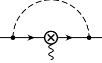
The leading contribution to $\Sigma=\Sigma(P)$ is of order $p^{2}$ – it stems from the term $4\,c_{1}M^{2}\bar{\psi}\psi$ contained in ${\cal L}^{(2)}_{N}$. The one loop graphs shown in fig. 4 are generated by ${\cal L}^{(1)}_{N}$, ${\cal L}^{(2)}_{N}$ and start

a		b		c

Figure 4: One loop graphs contributing to the self energy of the nucleon. The cross denotes a vertex from ${\cal L}_{N}^{(2)}$.

.

contributing at order $p^{3}$. Finally, there is a tree graph contribution from ${\cal L}^{(4)}_{N}$ (see eq. (2)):

$$\Sigma=-4\,c_{1}M^{2}+\Sigma_{a}+\Sigma_{b}+\Sigma_{c}+e_{1}M^{4}+O(p^{5})\;.$$

The explicit expressions for the loop contributions are obtained with the standard rules of relativistic perturbation theory:

$$\Sigma_{a}\! \!=\! \!\frac{3\,g_{A}^{2}}{4\,F^{2}}\,(m+P/\,)\left\{M^{2}I+(m-P/\,)\,P/\,I^{(1)}-\Delta_{N}\right\}\;,$$

$$\Sigma_{b}\! \!=\! \!\frac{3M^{2}\Delta_{\pi}}{F^{2}}\left\{2c_{1}-\frac{P^{2}}{m^{2}d}\,c_{2}-c_{3}\right\}\;,$$

$$\Sigma_{c}\! \!=\! \!-4c_{1}M^{2}\,\frac{\partial\Sigma_{a}}{\partial m}\;.$$

The mass insertion in graph c arises from the shift $m\rightarrow m_{2}=m-4c_{1}M^{2}$ in the nucleon propagator, generated by the term from ${\cal L}^{(2)}_{N}$ mentioned above. We could have replaced the mass in the free part of the Lagrangian by $m_{2}$, so that the graph 4c would then be absent.

The only difference to the standard evaluation of the graphs is that the loop integrals are regularized in a different manner. In particular, the full scalar self energy integral (fig. 4a) is replaced by the infrared part thereof, $I=I(P^{2},M^{2},m^{2})$ – we have discussed the properties of this function in detail in the preceding sections. The term $\Delta_{N}$ denotes the scalar nucleon propagator at the origin,

$$\Delta_{N}=\frac{1}{i}\int_{I}\frac{d^{d}k}{(2\pi)^{d}}\,\frac{1}{m^{2}-k^{2}-i\epsilon}\;.$$

In infrared regularization, that term vanishes, because it does not contain any infrared singularities (see section 6) :

$$\Delta_{N}=0\;.$$

For purely mesonic loops such as the one occurring in fig. 4b, there is no difference between dimensional and infrared regularization: The integral $\int_{I}d^{d}k$ coincides with the ordinary $d$-dimensional integral. The graph is proportional to the pion propagator at the origin, which we denote by $\Delta_{\pi}$,

$$\Delta_{\pi}=\frac{1}{i}\int_{I}\frac{d^{d}k}{(2\pi)^{d}}\,\frac{1}{M^{2}-k^{2}-i\epsilon}=2M^{2}\left(\bar{\lambda}+\frac{1}{16\pi^{2}}\,\mbox{ln}\,\frac{M}{m}\right)\;.$$

Finally, the integral $I^{(1)}$ may be expressed in terms of $I$ (see appendix B) :

$$I^{(1)}=\frac{1}{2P^{2}}\,\left\{(P^{2}-m^{2}+M^{2})\,I+\Delta_{\pi}-\Delta_{N}\right\}\;.$$

The same relation also holds in dimensional regularization.

The physical mass of the nucleon, which we denote by $m_{N}$, is determined by the position of the pole in the two-point-function. In view of the factor $m-P/\,$, the term $I^{(1)}$ does not contribute. Evaluating the quantity $I$ with the explicit expression in eq. (9), we obtain

$$m_{N}\! \!=\! \!m-4\,c_{1}M^{2}-\frac{3\,g_{A}^{2}\,M^{3}}{32\pi F^{2}}+k_{1}\,M^{4}\,\mbox{ln}\,\frac{M}{m}+k_{2}\,M^{4}+O(M^{5})\;,$$

$$k_{1}\! \!=\! \!-\frac{3}{32\pi^{2}F^{2}m}\left(g_{A}^{2}-8\,c_{1}m+c_{2}m+4\,c_{3}m\right)\;,$$ (34)

$$k_{2}\! \!=\! \!\bar{e}_{1}-\frac{3}{128\pi^{2}F^{2}m}\left(2\,g_{A}^{2}-c_{2}m\right)\;.$$

The formula agrees with the result of refs. [11, 12]. The bare constants $M$, $F$, $m$, $g_{A}$, $c_{1}$, $c_{2}$, $c_{3}$, $c_{4}$ remain finite when the regularization is removed, but $e_{1}$ contains a pole at $d=4$. The quantity $\bar{e}_{1}$ is the corresponding renormalized coupling constant at scale $\mu=m$ :

$$\bar{e}_{1}=e_{1}-\frac{3\bar{\lambda}}{2F^{2}m}\left(g_{A}^{2}-8\,c_{1}m+c_{2}m+4\,c_{3}m\right)\;.$$ (35)

11 Wave function renormalization

The wave function renormalization constant is the residue of the pole in the two-point-function and is determined by a derivative of the self energy with respect to the momentum,

$$Z^{-1}=1-\frac{\partial\Sigma}{\partial P/\,}\hskip 3.00003pt\rule[-8.99994pt]{0.20004pt}{23.00006pt}_{\;P/\,\,=\,m_{N}}\;.$$

With the above expression for $\Sigma$, which is valid to order $p^{4}$, we can extract the residue to accuracy $p^{3}$. The result,

$$Z=1-\frac{9\,M^{2}g_{A}^{2}}{2F^{2}}\left\{\bar{\lambda}+\frac{1}{16\pi^{2}}\left(\mbox{ln}\frac{M}{m}+\frac{1}{3}-\frac{\pi M}{2\,m}\right)\right\}+O(M^{4})\;,$$

is in agreement with those obtained within the heavy baryon formalism. For a detailed discussion of the latter, see ref. [12].

Note that the multiplicative renormalization $\psi^{ren}=Z^{-\frac{1}{2}}\psi$ does not render the two-point-function finite at $d=4$. The reason is the following. We may collect all of the correlation functions associated with $\psi$ and $\bar{\psi}$ by adding a term of the form $\bar{\eta}\,\psi+\bar{\psi}\,\eta$ to the effective Lagrangian, where $\eta(x)$ is an anticommuting external field. Such a term, however, breaks chiral symmetry: Under a chiral rotation, the field $\psi$ transforms with a matrix that involves the pion field. We cannot subject $\eta$ to the same rotation, because this field stays put when the meson variables are integrated out. So, off the mass shell, the correlation functions of the effective field are regularization dependent objects. In the context of the effective field theory, these are without significance – the field $\psi(x)$ merely represents a variable of integration.

Instead we could consider the field $\Psi=u\,\psi_{R}+u^{\dagger}\,\psi_{L}$, which does transform with a factor that is independent of the meson field: $\Psi_{R}\rightarrow V_{R}\,\Psi_{R},$ $\Psi_{L}\rightarrow V_{L}\,\Psi_{L}$. Accordingly, the counter terms needed to renormalize the quantum fluctuations generated by the term $\bar{\eta}\,\Psi+\bar{\Psi}\,\eta$ are chirally invariant. In contrast to the correlation functions of $\psi$, those of $\Psi$ can unambiguously be worked out. Indeed, these variables are relevant for the low energy analysis of QCD operators that are formed with three quark fields and carry the quantum numbers of the nucleon: The leading term in the effective field theory representation of such an operator is a multiple of $\Psi$.

The main point is that the correlation functions of $\psi$ do not represent physical quantities. The graphs for say the scalar form factor or the nucleon mass also involve nucleons propagating off the mass shell, but the result is uniquely determined by the Lagrangian: The low energy representation of these quantities in terms of the renormalized coupling constants is independent of the regularization used. The one for the correlation functions of the effective field is unambiguous only on the mass shell. On-shell matrix elements such as form factors or scattering amplitudes may be obtained by extracting the residues of the relevant poles in suitable correlation functions – in that connection, only the on-shell properties matter.

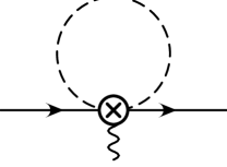
12 Scalar form factor to order $p^{4}$

In section 3, we considered the low energy representation of the scalar form factor to $O(p^{3})$. We now extend that representation to the next order of the expansion (for an analogous calculation of the scalar form factors within SU(3), based on HB $\chi$PT, see ref. [18]). For this purpose, we treat the quark masses $m_{u},\,m_{d}$ as external fields and calculate the response of the transition amplitude $\langle N(P^{\prime},s^{\prime})\,\mbox{out}|N(P,s)\,\mbox{in}\rangle$ to a local change in these fields. Within the effective theory, the transition amplitude may be worked out by treating the term $\chi$ in the effective Lagrangian as a space-time dependent quantity and evaluating the two-point-function $\langle 0\;\mbox{out}|T\psi(x)\,\bar{\psi}(y)|\,0\;\mbox{in}\rangle$ in the presence of this external field: The transition amplitude is determined by the residue of the double pole occurring in the Fourier transform of this quantity at $P^{2}=m_{N}^{2}$, $P^{\prime\,2}=m_{N}^{2}$. To extract the residue, we amputate the external nucleon legs, evaluate the remainder at $P^{2}=P^{\prime\,2}=m_{N}^{2}$ and multiply the result with the wave function renormalization constant $Z$.

12.1 Evaluation of the graphs

The tree graph contributions from ${\cal L}_{N}^{(2)}$ and ${\cal L}_{N}^{(4)}$ read:

$$\sigma_{tree}=Z\,(-4c_{1}M^{2}+2\,e_{1}M^{4}+e_{2}M^{2}t)\;.$$

The one loop graphs are shown in fig. 5.

a		b		c

d		e

Figure 5: The loop graphs contributing to the scalar form factor at $O(p^{4})$.

All of these, except the one in fig. 5a represent contributions of $O(p^{4})$. When performing the perturbative calculation, it is convenient to include the term $4\,c_{1}M^{2}\bar{\psi}\,\psi$ in the free part of the Lagrangian, replacing $m$ by $m_{2}=m-4\,c_{1}M^{2}$. The nucleons occurring in the various graphs then propagate with $m_{2}$. Note that the difference $m^{2}-P^{2}$ represents a quantity of order $p$. In the propagator, the shift $m\rightarrow m_{2}$ thus generates a first order correction. The distinction between $m$, $m_{2}$ and $m_{N}$ only matters in the triangle diagram 5a. In fact, graph 5b represents the change occurring in this diagram if $m$ is replaced by $m_{2}$ – this graph is absent if the mass insertion from $c_{1}$ is included in the free part of the Lagrangian. In view of $m_{N}-m_{2}=O(p^{3})$ we may also replace the factors of $m_{N}$ arising from the matrix elements $\bar{u}^{\prime}P/\,u$ and $\bar{u}^{\prime}P/\,^{\prime}u$ by $m_{2}$. The contributions from the one loop diagrams then take the form:

$$\!\sigma_{a}+\sigma_{b}=-\frac{3M^{2}g_{A}^{2}}{2F^{2}}\,\{4m^{3}I_{21}^{(1)}(t)-m\,J(t)\}\rule[-3.99994pt]{0.0pt}{15.00002pt}_{m\rightarrow m_{2}}\;,$$

$$\!\sigma_{c}=-\frac{6\,c_{1}M^{4}}{F^{2}}\,J(t)-\frac{3\,c_{2}M^{2}}{8F^{2}m^{2}}\,\left\{2\,t\,(4m^{2}-t)\,J^{(1)}(t)-2\,t^{2}J^{(2)}(t)+t^{2}J(t)\right\}$$

$$\!\hskip 20.00003pt-\frac{3\,c_{3}M^{2}}{2F^{2}}\,\left\{(t-2M^{2})\,J(t)+2\,\Delta_{\pi}\right\}\;,$$

$$\!\sigma_{d}=\frac{6\,c_{1}M^{2}}{F^{2}}\,\Delta_{\pi}\;,$$

$$\!\sigma_{e}=\frac{3\,c_{1}g_{A}^{2}M^{2}}{F^{2}}\,\left\{4M^{2}m^{2}I_{12}(t)-4m^{2}I^{(1)}(m^{2})+\Delta_{\pi}\right\}\;.$$

The notation is specified in appendix B. With the relations given there, the various invariants may be expressed in terms of the basic functions $J(t)$, $I(s)$, $I_{21}(t)$ and $I_{12}(t)$. The individual terms entering the combination $4m^{3}I_{21}^{(1)}(t)-m\,J(t)$ are of order $p^{0}$, but the leading terms cancel: The low energy expansion of $\sigma_{a}$ only starts at $O(p^{3})$, in accord with the counting of powers in graph 5a. Hence we may ignore the difference between $m_{2}$ and $m$ in the above expression.

The loop graphs contain divergences proportional to $M^{4}$ and to $M^{2}t$, respectively. The renormalization (35) of the coupling constant $e_{1}$ removes the first one. The second one requires the following renormalization of $e_{2}$:

$$\bar{e}_{2}=e_{2}+\frac{1}{2F^{2}m}\left\{3\,g_{A}^{2}+c_{2}m+6\,c_{3}m\right\}\bar{\lambda}\;.$$

12.2 Result

We write the result for $\sigma(t)=\sigma_{tree}+\sigma_{a}+\sigma_{b}+\sigma_{c}+\sigma_{d}+\sigma_{e}$ in the form

$$\sigma(t)=\sigma+\tilde{\sigma}(t)\;,$$

where $\sigma\equiv\sigma(0)$ represents the value of the form factor at the origin and is referred to as the $\sigma$-term. According to the Feynman-Hellmann theorem, this term represents the derivative of the nucleon mass with respect to the quark masses $m_{u}$, $m_{d}$, or, equivalently,

$$\sigma=M^{2}\,\frac{\partial\,m_{N}}{\partial M^{2}}\;.$$

Indeed, the sum of the contributions from the various graphs agrees with the derivative of the formula (10) for the nucleon mass.

For the remainder, the calculation yields:

$$\tilde{\sigma}(t)\! \!=\! \!\frac{3\,g_{A}^{2}M^{2}m}{4F^{2}}\,\{(t-2M^{2})\,\bar{I}_{21}(t)+2M^{2}\bar{I}_{21}(0)\}$$

$$\!+\{k_{3}\,M^{4}+k_{4}\,M^{2}t\}\,\bar{J}(t)+k_{5}\,M^{2}t+O(p^{5})\;,$$

$$k_{3}\! \!=\! \!-\frac{1}{F^{2}}\left\{6\,c_{1}-c_{2}-3\,c_{3}\right\}\;,$$

$$k_{4}\! \!=\! \!-\frac{1}{8F^{2}m}\left\{3\,g_{A}^{2}+2\,c_{2}m+12\,c_{3}m\right\}\;,$$

$$k_{5}\! \!=\! \!-\frac{1}{8\pi^{2}}\,k_{4}\,\mbox{ln}\,\alpha+\frac{1}{384\pi^{2}F^{2}m}\left\{9\,g_{A}^{2}+2\,c_{2}m+36\,c_{3}m\right\}+\bar{e}_{2}\;.$$

The only difference to the result of an analogous calculation in HB $\chi$PT is that the representation for the function $\bar{I}_{21}(t)$ given in appendix B also covers the vicinity of $t=4M^{2}$, where the heavy baryon representation fails. The value of $\sigma(t)$ at the Cheng-Dashen point $t=2M^{2}$ was given earlier, in ref. [19] – our expression confirms this result.

12.3 Unitarity

Unitarity offers an instructive test of the momentum dependence. Within the effective theory, the contributions from intermediate states containing more than two pions only show up at three loop order. Hence the representation obtained for the form factor must obey the elastic unitarity relation [20]

$$\mbox{Im}\,\sigma(t)=\theta(t-4\,M_{\pi}^{2})\;\frac{3\,\sqrt{t-4\,M_{\pi}^{2}}}{2\,\sqrt{t}\;(4m_{N}^{2}-t)}\;\sigma_{\pi}^{\star}(t)\,f^{0}_{+}(t)+O(p^{7})\;,$$ (37)

where $\sigma_{\pi}(t)$ is the form factor associated with the $\sigma$-term of the pion,

$$\sigma_{\pi}(t)=\langle\pi^{0}(p^{\prime})|\hat{m}\,(\bar{u}\,u+\bar{d}\,d)|\pi^{0}(p)\rangle$$

and $f^{0}_{+}(t)$ is the t-channel $I=J=0$ partial wave amplitude of $\pi N$ scattering.

To calculate the left hand side of the unitarity condition, we recall that the function $\bar{I}_{21}(t)$ represents the renormalized infrared part of the triangle integral $\gamma(t)$ introduced in section 3. At any finite order of the low energy expansion, the difference between the infrared part and the full integral is a polynomial, so that $\mbox{Im}\,\bar{I}_{21}(t)=\mbox{Im}\,\gamma(t)$. The explicit expression was given in eq. (5). For $\bar{J}(t)$, the imaginary part reads

$$\mbox{Im}\,\bar{J}(t)=\theta(t-4M^{2})\;\frac{\sqrt{t-4M^{2}}}{16\pi\sqrt{t}}\;.$$

The quantities on the right hand side of the unitarity condition are needed only at tree level, where $\sigma_{\pi}(t)=M^{2}$. The corresponding approximation for the $\pi N$ scattering amplitude is given in appendix C. The comparison shows that the representation obtained for the form factor indeed obeys the unitarity condition, up to contributions that are beyond the accuracy of a one loop calculation.

12.4 Value at the Cheng-Dashen point

The low energy theorem that underlies determinations of the $\sigma$-term from $\pi N$ data relates the scattering amplitude to the scalar form factor at the Cheng-Dashen point, where $t=2M_{\pi}^{2}$. It is therefore of interest to evaluate the difference

$$\Delta_{\sigma}=\sigma(2M_{\pi}^{2})-\sigma(0)$$

with the above representation of the form factor. The result is of the form

$$\Delta_{\sigma}\! \!=\! \!\Delta_{1}\,M^{3}+\Delta_{2}\,M^{4}\,\mbox{ln}\,\frac{M}{m}+\Delta_{3}\,M^{4}+O(M^{5})\;,$$

$$\Delta_{1}\! \!=\! \!\frac{3\,g_{A}^{2}}{64\pi F^{2}}\;.$$

The terms of order $M^{4}$ involve the coupling constants of ${\cal L}_{N}^{(2)}$:

$$\Delta_{2}\! \!=\! \!\frac{3\,g_{A}^{2}}{16\pi^{2}F^{2}m}+\frac{c_{2}}{16\pi^{2}F^{2}}+\frac{3\,c_{3}}{8\pi^{2}F^{2}}\;,$$ (38)

$$\Delta_{3}\! \!=\! \!\frac{3(2+\pi)\,g_{A}^{2}}{128\pi^{2}F^{2}m}-\frac{3(4-\pi)\,c_{1}}{16\pi^{2}F^{2}}+\frac{(14-3\pi)\,c_{2}}{192\pi^{2}F^{2}}+\frac{3\,c_{3}}{16\pi^{2}F^{2}}+2\,\bar{e}_{2}\;.$$

To express these in terms of observable quantities, we compare the tree graphs for the $\pi N$ scattering amplitude generated by ${\cal L}_{N}^{(1)}+{\cal L}_{N}^{(2)}$ with the subthreshold expansion of Höhler and collaborators [21] (see appendix C). Since that comparison allows us to determine the effective coupling constants only up to corrections of order $M$, we denote the resulting estimates by $c_{i}^{(0)}$:

$$c_{1}^{(0)}\! \!=\! \!-\frac{F^{2}}{4M^{2}}\,\left\{d_{00}^{+}+2M^{2}\,d_{01}^{+}\right\}\;,\hskip 30.00005ptc_{2}^{(0)}=\frac{F^{2}}{2}\;d_{10}^{+}$$ (39)

$$c_{3}^{(0)}\! \!=\! \!-F^{2}\,d_{01}^{+}\;,\hskip 102.00012ptc_{4}^{(0)}=\frac{1}{2m}\left\{F^{2}\,b_{00}^{-}-\mbox{$\frac{1}{2}$}\right\}\;.$$

The above expressions for $\Delta_{2}$ and $\Delta_{3}$ then take the form

$$\Delta_{2}\! \!=\! \!\frac{3\,g_{A}^{2}}{16\pi^{2}F^{2}m}+\frac{d_{10}^{+}}{32\pi^{2}}-\frac{3\,d_{01}^{+}}{8\pi^{2}}\;,$$

$$\Delta_{3}\! \!=\! \!\frac{3(2+\pi)\,g_{A}^{2}}{128\pi^{2}F^{2}m}+\frac{3(4-\pi)\,d_{00}^{+}}{64\pi^{2}M^{2}}+\frac{(14-3\pi)\,d_{10}^{+}}{384\pi^{2}}+\frac{3(2-\pi)\,d_{01}^{+}}{32\pi^{2}}+2\bar{e}_{2}\;.$$

The difference between $F$, $F_{\pi}$ and $M$, $M_{\pi}$ is beyond the accuracy of the representation (12). We replace $F$ by $F_{\pi}=92.4\,\mbox{MeV}$ and use the mass of the charged pion. For the same reason, we may identify the bare coupling constant $g_{A}$ with the experimental value $g_{A}=1.267\pm 0.0035$ [22]. Using the values of the subthreshold coefficients quoted in appendix C, we then obtain $\Delta_{1}\,M^{3}=7.6\,\mbox{MeV}$, $\Delta_{2}\,M^{4}\,\mbox{ln}\,\alpha=7.8\,\mbox{MeV}$ and $(\Delta_{3}-2\,\bar{e}_{2})\,M^{4}=-1.4\,\mbox{MeV}$. These terms add up to

$$\Delta_{\sigma}=14.0\,\mbox{MeV}+2\,M^{4}\bar{e}_{2}\;,$$

to be compared with the result of the dispersive calculation of ref. [20]:

$$\Delta_{\sigma}=15.2\pm 0.4\;\mbox{MeV}\;.$$ (40)

The comparison shows that the contribution from the coupling constant $\bar{e}_{2}$ is small, as it should be.

The above calculation resolves an old puzzle: The leading term in the chiral expansion of $\Delta_{\sigma}$ – the one of order $M^{3}$ – accounts for only half of the result. The terms of order $M^{4}$ are numerically of the same size, because they are enhanced by a chiral logarithm. The underlying physics can be sorted out by noting that the elastic unitarity condition (37) leads to the representation

$$\Delta_{\sigma}\! \!=\! \!\int_{4M_{\pi}^{2}}^{\infty}dt\,n(t)\,\sigma_{\pi}^{\star}(t)\,f^{0}_{+}(t)\;,$$ (41)

$$n(t)\! \!=\! \!\frac{3M_{\pi}^{2}\,\sqrt{t-4\,M_{\pi}^{2}}}{\pi\,t^{\frac{3}{2}}\,(t-2M_{\pi}^{2})\,(4m_{N}^{2}-t)}\;.$$

The one loop calculation discussed above replaces the pion $\sigma$-term by the first term in the chiral series, $\sigma_{\pi}(t)\rightarrow M_{\pi}^{2}$. The contribution proportional to $g_{A}^{2}$ represents the value of the dispersion integral that results if the partial wave amplitude is replaced by the Born approximation $f_{\!B+}^{\,0}(t)=O(p)$, given in eq. (C.2). The remainder is dominated by the coupling constant $c_{3}$, which generates a polynomial contribution to the partial wave amplitude: $f_{+}^{0}(t)_{c_{3}}=(2M^{2}-t)\,c_{3}\,m^{2}/4\pi F^{2}=O(p^{2})$.

The tree approximation for $f_{+}^{0}(t)$ is shown in fig. 6,

\psfrag{x}[lB]{\large$t$ }\psfrag{y}[lb]{\large$nf_{+}^{0}$}\includegraphics[width=289.07999pt]{sigmaFigur.eps}

Figure 6: The $t$-channel $I=J=0$ partial wave $f_{+}^{0}(t)$. The normalization factor $n$ is chosen such that $\Delta_{\sigma}$ is the area under the curve (dotted: Born approximation, dash-dotted: tree graphs of ${\cal L}_{N}^{(1)}+{\cal L}_{N}^{(2)}$, full: dispersion theory, all quantities in units of $M_{\pi}$).

together with the Born term (tree graph from ${\cal L}_{N}^{(1)}$ alone). To indicate the weight in the dispersion integral (41), we plot the corresponding contributions to the quantity $n(t)\,f_{+}^{0}(t)$. We also depict the result of the dispersive evaluation described in ref. [20], which includes the higher orders of the chiral series and is therefore complex – the curve shown represents the quantity $n(t)\,|f^{0}_{+}(t)|$. Qualitatively, the picture is quite similar to the one found for the imaginary part of the scalar form factor of the pion, $\mbox{Im}\,\sigma_{\pi}(t)$: The higher order effects tend to amplify the leading order terms also in that case [23, 24].

The figure demonstrates that, at low energies, the tree approximation to the scattering amplitude provides a rather decent representation. The Born term alone, however, only dominates in the immediate vicinity of $t=4M_{\pi}^{2}$, where it exhibits the peculiar structure discussed in section 4. For $\sqrt{t}>380\,\mbox{MeV}$, the contribution generated by the coupling constants $c_{1}$, $c_{2}$ and $c_{3}$ is more important than the one proportional to $g_{A}^{2}$.

Although the straightforward expansion of $\Delta_{\sigma}$ in powers of the quark masses is well-defined and can unambiguously be worked out, the first term of that series does not yield a decent approximation. The term arises from the infrared singularity generated by the Born approximation. On the one hand, the contributions from the second term of the chiral expansion are suppressed by one power of $M$, on the other, they are enhanced by a chiral logarithm – numerically, they are equally important.

12.5 The $\sigma$-term

Finally, we turn to the value of the form factor at $t=0$. The first four terms in the chiral expansion of the nucleon mass were given in eq. (10). The corresponding expansion for $\sigma\equiv\sigma(0)$ is of the form

$$\sigma=\sigma_{1}M^{2}+\sigma_{2}M^{3}+\sigma_{3}M^{4}\,\mbox{ln}\,\frac{M}{m}+\sigma_{4}M^{4}+O(M^{5})\;.$$ (42)

The coefficients follow from the Feynman-Hellmann theorem:

$$\sigma_{1}\! \!=\! \!-4\,c_{1}\;,$$ (43)

$$\sigma_{2}\! \!=\! \!-\frac{9\,g_{A}^{2}}{64\pi F^{2}}\;,$$

$$\sigma_{3}\! \!=\! \!-\frac{3}{16\pi^{2}F^{2}\,m}\,(g_{A}^{2}-8\,c_{1}m+c_{2}m+4\,c_{3}m)\;,$$

$$\sigma_{4}\! \!=\! \!-\frac{3}{64\pi^{2}F^{2}\,m}\,(3\,g_{A}^{2}-8\,c_{1}m+4\,c_{3}m)+2\,\bar{e}_{1}\;.$$

The tree approximation (39) for the effective coupling constants $c_{1}$, $c_{2}$, $c_{3}$ suffices to work out the numerical values of $\sigma_{2}$, $\sigma_{3}$, as well as the corresponding contribution to $\sigma_{4}$. With the values of the subthreshold coefficients quoted in appendix C, we obtain $\sigma_{2}M^{3}\!=\!-23\,\mbox{MeV}$, $\sigma_{3}M^{4}\,\mbox{ln}\,\alpha\!=\!-9\,\mbox{MeV}$, $(\sigma_{4}-2\,\bar{e_{1}})\,M^{4}\!=\!0.9\,\mbox{MeV}$. To evaluate $\sigma_{1}$ in an analogous manner, we need a more accurate determination of $c_{1}$, but we may instead take the experimental value $\sigma\!=\!45\,\mbox{MeV}$ from ref. [20]. This leads to the estimate $\sigma_{1}M^{2}+2\,\bar{e}_{1}M^{4}\!=\!76\,\mbox{MeV}$, subject to an uncertainty of about $8\,\mbox{MeV}$.

These numbers show that the expansion of $\sigma$ in powers of the quark masses contains a large contribution from the infrared singularity generated by the Born term, $\sigma_{2}M^{3}$. At the next order of the expansion, there is a logarithmic infrared singularity, $\sigma_{3}M^{4}\,\mbox{ln}\,\alpha$. The comparison with the leading term $\sigma_{1}M^{2}$ shows that this effect is of the size typical for chiral logarithms. The main difference to the situation encountered in the mesonic sector is that the expansion contains odd as well as even powers of $p$. If the series is truncated at order $p^{3}$, we must expect a less accurate representation than the one obtained in the mesonic sector at one loop.

The determination of the coupling constant $c_{1}$ to the accuracy needed here requires a calculation of the $\pi N$ scattering amplitude to order $p^{4}$ and is beyond the scope of the present paper. We can, however, study the effects generated by the leading infrared singularities in the values of the effective coupling constants. For this purpose, we make use of the results reported in ref. [1, 6, 7], where the scattering amplitude is evaluated to order $p^{3}$. The formulae for the coefficients of the subthreshold expansion given in ref. [7, 25] imply that the corrections of $O(p^{3})$ generate the following shifts in the values of the effective coupling constants:

$$c_{i}^{(1)}\! \!=\! \!c_{i}^{(0)}+\delta c_{i}$$ (44)

$$\delta c_{1}\! \!=\! \!-\frac{59\,g_{A}^{2}}{1536\pi F^{2}}\,M\;,\hskip 45.00006pt\delta c_{2}=\frac{5\,g_{A}^{4}+4}{64\pi F^{2}}\,M\;,$$

$$\delta c_{3}\! \!=\! \!-\frac{g_{A}^{2}(48\,g_{A}^{2}+77)}{768\pi F^{2}}\,M\;,\hskip 20.00003pt\delta c_{4}=\frac{g_{A}^{2}(g_{A}^{2}+1)}{16\pi F^{2}}\,M\;.$$

As a check, we have applied the method discussed in section 6 to the loop integrals that occur in the representation of the scattering amplitude given in ref. [1]. In the vicinity of the point $\nu=t=0$, the chiral expansion converges for all of these (see appendix B). The result confirms the formulae for the coefficients of the subthreshold expansion quoted above and thus also corroborates the expressions (44) for the first order shifts in the effective coupling constants. The one for $c_{1}$ allows us to establish the relation between the $\sigma$-term and the subthreshold coefficients to accuracy $p^{3}$:

$$\sigma=F_{\pi}^{2}\,(d_{00}^{+}+2M_{\pi}^{2}d_{01}^{+})+\frac{5\,g_{A}^{2}M_{\pi}^{3}}{384\pi F_{\pi}^{2}}+O(M_{\pi}^{4})\;,$$

to be compared with the prediction at tree level, $\sigma=F_{\pi}^{2}\,(d_{00}^{+}+2M_{\pi}^{2}d_{01}^{+})$, where the third term is missing. Numerically, the shift amounts to only $2.1\,\mbox{MeV}$: In the relation between the observables $\sigma$, $d_{00}^{+}$ and $d_{01}^{+}$, the effects generated by the leading infrared singularities are an order of magnitude smaller than those seen in the chiral expansion of $\sigma$. This demonstrates that the large infrared singular contribution that occurs in the chiral expansion of the $\sigma$-term at $O(M^{3})$ also appears in the $\pi N$ scattering amplitude – the relevant combination of subthreshold coefficients picks up nearly the same contribution. Note that the magnitude of the $\sigma$-term as such is not at issue here. For the values of the coefficients $d_{00}^{+}$, $d_{01}^{+}$ given in ref. [21], the tree level and one loop results for $\sigma$ are $50$ and $52\,\mbox{MeV}$, respectively. We could have used a somewhat different input, for instance one for which the outcome for the $\sigma$-term is 45 MeV – the difference between the tree and one loop approximations would be the same.

13 Discussion

13.1 Reordering of the perturbation series

The fact that the bulk of the infrared singular contributions occurring in the chiral expansion of the nucleon mass and of the $\sigma$-term merely amounts to a shift of the bare parameters was noted long ago [26]. In the preceding section, we listed the change in the effective coupling constants $c_{1},c_{2},c_{3},c_{4}$ generated by the infrared singularities at $O(p^{3})$ and pointed out that, in the relations between the observable quantities considered, these singularities nearly cancel. We expect a similar, albeit less dramatic reduction also to occur in other quantities of physical interest. Some of the fluctuations seen in the published results for the threshold parameters of $\pi N$ scattering, for instance, merely reflect the fact that the expansion of the various observables in powers of the quark masses contain large contributions from infrared singularities.

A more significant comparison of the results obtained at tree level and at one loop results if one considers the predictions of the effective theory: Instead of comparing the contributions arising in the chiral expansion of a given observable at various orders of the expansion, one may compare the relations between observable quantities which follow at tree level with those obtained at one loop. The effective coupling constants entering the one loop result are different from those relevant at tree level. The tree level values are the best choice for the representation of the scattering amplitude to $O(p^{2})$, those in eq. (44) are relevant for the improved representation of this amplitude that accounts for the terms of $O(p^{3})$.

The elimination of the coupling constants in favour of physical quantities amounts to a reordering of the perturbation series. In more explicit terms, the reordering we are advocating here is the following (we restrict ourselves to a discussion to one loop). The perturbation series relies on a decomposition of the effective Lagrangian into a leading term and a perturbation,

$${\cal L}_{N}\! \!=\! \!{\cal L}_{0}+{\cal L}_{1}\;.$$

The standard ordering results if ${\cal L}_{0}$ is identified with the first two terms of the derivative expansion. We argue that the decomposition

$${\cal L}_{0}\! \!=\! \!{\cal L}^{(1)}_{N}+{\cal L}^{(2)}_{N}\,\rule[-6.00006pt]{0.29999pt}{15.00002pt}_{\;c_{i}\rightarrow c_{i}^{(0)}}$$

$${\cal L}_{1}\! \!=\! \!{\cal L}^{(3)}_{N}+{\cal L}^{(4)}_{N}+{\cal L}^{(2)}_{N}\,\rule[-6.00006pt]{0.29999pt}{15.00002pt}_{\;c_{i}\rightarrow\delta c_{i}}\;,$$

with $\delta c_{i}=c_{i}-c_{i}^{(0)}$, is a better choice, because it reduces the magnitude of the perturbation ${\cal L}_{1}$. Like for the standard bookkeeping, an evaluation of the various observables to $O(p^{2})$ requires the calculation of the tree graphs belonging to ${\cal L}_{0}$; for a representation to $O(p^{4})$, we need to add the tree graphs of ${\cal L}_{1}$ as well as the one loop graphs of ${\cal L}_{0}$.

Two modifications occur when the perturbation series is extended from $O(p^{2})$ to $O(p^{4})$: new graphs and the change $\delta c_{i}$ in the values of the coupling constants (the explicit expressions for the latter in eq. (44) account for the shifts of order $\delta c_{i}=O(M)$, but do not include those of order $M^{2}$). As discussed above, the two effects partly cancel. In the above bookkeeping, the change $\delta c_{i}$ is booked among the corrections, on the same footing as the contributions from the loop graphs, which both affect the observables and are responsible for the shift in the coupling constants. The cancellations between the two types of contributions thus tend to reduce the magnitude of the perturbations generated by ${\cal L}_{1}$.

At first sight, the claim that the values of the coupling constants depend on the order at which the perturbation series is considered, may appear to contradict the fact that these constants represent perfectly well-defined quantities that determine the chiral expansion coefficients of the various observables. As is well known, the results found for these coefficients on the basis of a calculation to some given order of chiral perturbation theory represent low energy theorems that remain strictly valid if the expansion is carried to higher orders. We do not put this into question, but merely emphasize that the result obtained for the values of the coupling constants does depend on the order to which the perturbation series is worked out.

To illustrate the need for a distinction between the coupling constants as such and their values at a given order of the perturbation series, we again consider the quantity $\Delta_{\sigma}$ and focus on the chiral logarithm contained therein, $\Delta_{2}M^{4}\,\mbox{ln}\,\alpha$. The term arises from the infrared singularity occurring at the lower end of the dispersion integral (41). According to eq. (38), the coefficient $\Delta_{2}$ contains a piece that is proportional to the coupling constants $c_{2}$ and $c_{3}$. It arises from the contribution to the partial wave $f^{0}_{+}(t)$ that is generated by the tree graphs of ${\cal L}^{(2)}_{N}$. Hence the coupling constants relevant for an evaluation of $\Delta_{2}$ are those pertaining to the tree level representation of the scattering amplitude. If we were to calculate $\Delta_{2}$ with the improved values of the coupling constants that follow from the relations (44), we would in effect be using a tree level representation for $f^{0}_{+}(t)$ with the wrong coupling constants. The point here is that the same one loop graphs that give rise to a change in the values of $c_{2}$, $c_{3}$ also modify the partial wave amplitude. Since a substantial fraction of the infrared singularities occurring at $O(p^{3})$ affects the term $\Delta_{\sigma}$ and the scattering amplitude in the same way, it does not make sense to account for one of the changes without accounting for the other.

In a certain sense, the odd and even powers of the chiral series lead a life of their own. The quantity $\Delta_{\sigma}$ illustrates the fact that the leading terms in both of the subseries need to be investigated in order to arrive at a significant result. To our knowledge, the available one loop results for the $\pi N$ scattering amplitude account for the expansion only to $O(p^{3})$. It will be very interesting to compare the predictions that follow from the representation of the amplitude to $O(p^{4})$ with those obtained from the same experimental input at tree level.

The problem also occurs in the mesonic sector. The infrared singularities are weaker there, because the expansion only involves even powers of $p$. At the precision reached with a two loop calculation, however, the need for a distinction between the coupling constants as such and the values found at a given order of the perturbation series manifests itself quite clearly. As discussed in refs. [27, 28], for instance, inconsistencies may arise if the two loop representation for the $\pi\pi$ scattering amplitude is evaluated with the values of the coupling constants $\ell_{1}$, $\ell_{2}$ obtained on the basis of a one loop calculation from $K_{e_{4}}$ decay.

13.2 The role of the $\Delta(1232)$

The occurrence of a chiral logarithm explains why an evaluation of $\Delta_{\sigma}$ to order $M^{3}$ does not yield a decent approximation for this quantity. The coefficient of the logarithm involves the combination $c_{2}+6\,c_{3}$ of effective coupling constants, which is dominated by $c_{3}$. It is understood why the value of this coupling constant obtained from low energy $\pi N$ phenomenology is large: This constant receives an important contribution from the singularities generated by the $\Delta(1232)$. In fact, it was noted in ref. [29] that a calculation of the scalar form factor that explicitly includes the $\Delta$ degrees of freedom yields a result for $\Delta_{\sigma}$ that is consistent with the one obtained from dispersion theory.

The role of this state for the low energy structure in the baryonic sector is discussed in detail in the literature [8, 21, 29, 30, 31]. For a recent review, in particular also of the small scale expansion that allows one to analyze the extension of the effective theory in a controlled manner, we refer to [32]. The extended theory is compared with the framework used in the preceding sections in appendix D, where we also estimate the contributions to the effective coupling constants that are generated by the $\Delta$.

For the quantities analyzed in the present paper, it is not essential whether the $\Delta$ is incorporated as a dynamical variable in the effective Lagrangian or whether the effects generated by this state are accounted for only indirectly, through the values of the effective coupling constants: In the domain studied here, the graphs describing the exchange of a $\Delta$ are adequately described by those terms of the chiral expansion that occur up to and including $O(p^{4})$.

In the Mandelstam plane, the point around which the chiral expansion is performed corresponds to $s_{0}=m^{2}+M^{2}$, $t=0$. The expansion of the resonance denominators is controlled by the ratio $x=(s-s_{0})^{2}/(m_{\Delta}^{2}-s_{0})^{2}$. For small values of $s-s_{0}$ and $t$, in particular near the Adler zero and for quantities like $\sigma(0)$ or $\sigma(2M^{2})$, the expansion rapidly converges. At the threshold, where $x=4M^{2}m^{2}/(m_{\Delta}^{2}-m^{2}-M^{2})^{2}\simeq 0.18$, the expansion of the resonance denominators is still under good control. For higher energies, however, the singularities generated by the $\Delta$ must explicitly be accounted for to arrive at a decent representation of the scattering amplitude.

In the mesonic sector, the $\rho$ plays an analogous role. Remarkably, as far as the expansion of the resonance denominators is concerned, the convergence radius is roughly the same: $m_{\Delta}^{2}-m^{2}-M^{2}\simeq m_{\rho}^{2}-2M^{2}$ (the left hand side is even a little larger). The two Mandelstam triangles, however, are of very different size: The one relevant for $\pi\pi$ scattering is smaller by the factor $M/m$, so that the threshold is much closer to the Adler zero. At the threshold, the parameter that controls the expansion of the term $1/(m_{\rho}^{2}-s)$ is very small indeed: $x=4M^{4}/(m_{\rho}^{2}-2M^{2})^{2}\simeq 0.005$. In the mesonic sector, an effective theory that does not explicitly account for this singularity yields meaningful results even well above threshold.

13.3 Comparison with the static model

It is instructive to compare the framework discussed above with the earliest version of an effective field theory for the baryons, the static model. This model is characterized by the Hamiltonian [33]:

$$H=\int\!d^{3}\!x\,\frac{1}{2}\left\{\dot{\mbox{\boldmath$\pi$}}^{\,2}+{\nabla\mbox{\boldmath$\pi$}}^{\,2}+{M_{\pi}^{2}\,\mbox{\boldmath$\pi$}}^{\,2}\right\}+\int\!\!d^{3}\!x\,\frac{g_{A}}{2F_{\pi}}\,\rho(\vec{x})\,\psi^{\dagger}\,(\mbox{\boldmath$\sigma$}\cdot\nabla)\,(\mbox{\boldmath$\pi$}\cdot\mbox{\boldmath$\tau$})\,\psi\;.$$

The nucleon is kept fixed at the origin, $\psi(x)\rightarrow\psi(t)$. The corresponding four-dimensional space of states is spanned by vectors that differ in the spin and isospin quantum numbers – the operator $\psi^{\dagger}\ldots\psi$ generates transitions between these. The result for the self energy of the nucleon reads

$$E=-\frac{3\,g_{A}^{2}}{32\pi F_{\pi}^{2}}\int\!\!d^{3}\!xd^{3}\!y\,\,\nabla\rho(\vec{x})\cdot\nabla\rho(\vec{y})\;\frac{e^{-M_{\pi}|\vec{x}-\vec{y}\,|}}{|\vec{x}-\vec{y}\,|}\;.$$

The function $\rho(\vec{x})$ is normalized to $\int\!d^{3}\!x\,\rho(\vec{x})=1$ – it describes the structure of a nucleon that is stripped of its meson cloud.

In the relativistic formulation of the effective theory, the nucleon is represented as a point particle, $\rho(\vec{x})\rightarrow\delta(\vec{x})$, and the leading contributions to the self energy of the nucleon arise from one loop graphs. To compare the expressions for the self energy, we note that in the static model, the expansion of the exponential yields the series $1-M_{\pi}r+\frac{1}{2}M_{\pi}^{2}r^{2}-\frac{1}{6}M_{\pi}^{3}r^{3}+\ldots$ The second term vanishes upon integration, so that the series takes the form $E=E_{1}+E_{2}M_{\pi}^{2}+E_{3}M_{\pi}^{3}+\ldots$ In our formulation of B $\chi$PT, only the infrared part of the loop integrals is retained, the remainder being absorbed in the effective coupling constants. In that language, the term $E_{1}$ is included in the bare mass $m$, while $E_{2}$ represents a contribution to the effective coupling constant $c_{1}$. The coefficient $E_{3}$ is independent of the shape of $\rho(\vec{x})$ and the value $E_{3}=-3\,g_{A}^{2}/32\pi F_{\pi}^{2}$ indeed reproduces the coefficient occurring in the chiral expansion (10) of the nucleon mass. At the next order of the expansion, however, the static model fails: The self energy $E$ does not contain a chiral logarithm. In fact, in the local limit $\rho(\vec{x})\rightarrow\delta(\vec{x})$, the expansion terminates at $O(M_{\pi}^{3})$. The deficiency arises because the model only accounts for the leading term ${\cal L}_{N}^{(1)}$ in the derivative expansion of the effective Lagrangian – the formula (43) shows that, in the static limit ($m\rightarrow\infty$), the nucleon mass does not contain a chiral logarithm if the coupling constants $c_{1},c_{2},c_{3}\in{\cal L}_{N}^{(2)}$ are turned off.

Quite a few other phenomena ($\pi N$ scattering, magnetic moments and electromagnetic form factors, pion photoproduction, Compton scattering, nuclear forces, for instance) were analyzed in detail within the static model, which provides a simple intuitive picture for the basic low energy features (for an excellent overview, we refer to the book of Henley and Thirring [33]). A comparison of the results obtained with the modern version of the effective theory with those found in this model would be most instructive.

13.4 Momentum space cutoff

The formulation of the effective theory in terms of pointlike nucleons has the advantage of being model independent. It systematically accounts for all contributions arising to a given order in the chiral expansion of the various observables. The price to pay is that the loop integrals cannot be interpreted directly in physical terms. The machinery does incorporate the finite extension of the nucleon, but only indirectly, through the effective coupling constants. A more intuitive picture of the meson cloud that does explicitly account for the finite size of the nucleon was proposed in ref. [26]. In that framework, the pointlike vertices are replaced by form factors, which in effect cut the virtual meson momenta off. The proposal is based on the static model, where the $\pi N$ interaction is also equipped with a form factor, given by the Fourier transform of the function $\rho(\vec{x})$. The motivation for introducing such a cutoff was that the matrix elements of the perturbations encountered in the extension of B $\chi$PT from SU(2) to SU(3) are large. It does not make much sense to truncate the straightforward expansion of the baryon masses in powers of $m_{u},m_{d}$ and $m_{s}$ at order $p^{3}$. The net effect of a cutoff is qualitatively similar to the one resulting from the reordering discussed above: It reduces the magnitude of those terms that are treated as perturbations.

The proposal is taken up in the recent literature [34]. In particular, the quantity $\Delta_{\sigma}$ is studied within that framework in ref. [35]. In the language of the dispersion relation (41), the calculation reported there essentially amounts to replacing the partial wave amplitude $f_{+}^{0}(t)$ by the Born term (dotted line in fig. 6) and cutting the dispersion integral off at moderate values of $t$. Such a calculation evidently yields a much smaller value for $\Delta_{\sigma}$ than the one that follows, either from dispersion theory or from the evaluation of the chiral perturbation series to order $p^{4}$. The analysis of section 12.4 shows that the contributions of order $p^{3}$ and $p^{4}$ are of a different origin. The terms of order $p^{4}$ are not properly accounted for by cutting off the virtual momenta in the one loop graphs of order $p^{3}$.

More generally, the problem with the approach proposed in ref. [26] is that it is model dependent. Moreover, introducing a cutoff in general ruins the Ward identities of chiral symmetry. The model independent method we are proposing does preserve the Ward identities as well as the infrared structure. The reordering of the perturbation series also leads to a more rapidly convergent expansion. It yet remains to be seen, however, whether this method will provide a coherent understanding of the mass spectrum of the baryon octet.

14 Conclusion

 1. We have shown that B $\chi$PT can be formulated in such a manner that both Lorentz invariance and chiral power counting are preserved at every stage of the calculation. The method relies on the fact that – for noninteger values of the dimension – the infrared singular parts of the loop graphs can unambiguously be separated from the remainder: They involve fractional powers of the chiral expansion parameters, while the remainder admits an ordinary Taylor series. The two parts are chirally invariant by themselves in the sense that they separately obey the Ward identities of chiral symmetry. This allows us to retain only the infrared singular parts of the loop integrals, absorbing the remainder in the coupling constants of the effective Lagrangian.

2. The calculations required by our method are nearly identical to those relevant within the relativistic formulation of the effective theory given in ref. [1]. The Lagrangian and the Feynman graphs are the same. The only difference is that the loop integrals are replaced by the corresponding infrared parts. At one loop order, this is achieved by extending one of the Feynman parameter integrations from the interval $0<z<1$ to the interval $0<z<\infty$.

3. We have shown that, in the sector with baryon number 1, the chiral expansion breaks down in certain regions of phase space. The nonrelativistic expansion that underlies HB $\chi$PT inherits this problem and also leads to technical difficulties of its own, related to the fact that the nonrelativistic expansion of infrared singularities is a rather subtle matter. A coherent heavy baryon representation only results if the insertions required by relativistic kinematics are summed up to all orders. The problem arises from the interchange of the loop integration with the nonrelativistic expansion, which is not always legitimate. The method we are proposing avoids these difficulties ab initio, because it does not rely on a nonrelativistic expansion of the loop integrals.

4. One of the advantages of chiral perturbation theory is that, at the algebraic level, the results are unambiguous. This implies that the chiral expansion of the representations obtained with the method proposed here must agree with the results of HB $\chi$PT, order by order – even in those cases where this expansion does not converge.

5. As our method avoids the nonrelativistic expansion of the vertices, the number of graphs to be evaluated is smaller than in HB $\chi$PT. The price to pay is that the simplifications offered by nonrelativistic kinematics cannot be made use of. As an example, we mention processes involving external photons, such as pion photoproduction. Bernard, Kaiser, Kambor and Meissner [3] have shown that, in the heavy baryon approach, many of the one loop graphs occurring in that context can be dropped: In the nonrelativistic limit and in the Coulomb gauge, vertices involving the coupling of photons to a nucleon line are suppressed. Since our method leads to the same power counting rules as the nonrelativistic expansion, we expect these simplifications to also apply within our framework, but a relativistic formulation of the corresponding selection rules yet remains to be given.

6. In the baryonic sector, the expansion involves odd as well as even powers of momenta. Most of the available calculations only account for the terms arising up to and including $O(p^{3})$. The corresponding representation for the observables of physical interest is inherently less accurate than the one obtained at one loop in the mesonic sector, which holds up to and including $O(p^{4})$. A full one loop calculation of the $\pi N$ scattering amplitude yet remains to be carried out.

7. We have illustrated our method with an evaluation of the $\sigma$-term and of the corresponding form factor to order $p^{4}$. The form factor can be expressed in terms of elementary functions throughout the low energy region. In the domain where the standard chiral expansion in powers of momenta and quark masses is convergent, the result agrees with the one obtained on the basis of HB $\chi$PT. The representation constructed in the present paper, however, also holds in the vicinity of $t=4\,M_{\pi}^{2}$, where the heavy baryon chiral perturbation series diverges.

8. The example of the form factor shows that the expansion of some of the observables in powers of the quark masses contains a large contribution from the infrared singularities generated by the Born term, proportional to $g_{A}^{2}M_{\pi}^{3}$. We have shown, however, that the bulk of this contribution is common to the $\sigma$-term and to the $\pi N$ scattering amplitude, so that it drops out when considering the predictions of the theory, i.e. the relations between the observables.

9. Although the straightforward expansion of the various observables in powers of momenta and quark masses is perfectly meaningful, it does not yield a suitable ordering of the perturbation series. We have proposed a model independent reordering of this series, which can also be performed in HB $\chi$PT. At least in the two cases considered in the present paper ($\sigma$-term and momentum dependence of the scalar form factor), the operation strongly reduces the magnitude of the corrections. To see whether or not this is a peculiarity of the observables considered here, it would be of interest to perform the operation with the known representation of the $\pi N$ scattering amplitude to $O(p^{3})$ [1, 6, 7, 8].

10. We have discussed the effects generated by the $\Delta(1232)$ in some detail. This state plays a role similar to the one of the $\rho$ in the mesonic sector: In the Mandelstam plane, the singularities associated with the $\Delta$ and the $\rho$ occur at about the same distance from the point around which the chiral expansion is performed. As far as the behaviour of the scattering amplitude in the vicinity of the Adler zero is concerned, or for quantities such as $\sigma(0)$ or $\sigma(2M^{2})$, the singularities generated by the $\Delta$ are adequately described by their contributions to the effective coupling constants.

11. The physical region of $\pi N$ scattering is further away from the Adler zero than the physical region of $\pi\pi$ scattering, by one power of $m/M$. Although, at the threshold, the singularities generated by the $\Delta$ may still be replaced by their contributions to the effective coupling constants, we must expect the perturbation series for the threshold parameters to converge less rapidly for $\pi N$ scattering than for $\pi\pi$ scattering.

12. In the experimentally accessible region, the $\Delta$ does play a prominent role. The work reported in ref. [37] indicates that, even in the vicinity of the resonance, a decent description of the observed behaviour of the scattering amplitude may be obtained by supplementing the tree graphs of a simple resonance model with unitarity corrections. It yet remains to be seen whether a systematic analysis of the extended effective theory that includes the $\Delta$ among the dynamical variables and incorporates chiral symmetry ab initio will allow us to establish direct contact with the wealth of experimental data.

13. The problems discussed in the present paper are not peculiar to the nucleons, but occur whenever the effective theory contains degrees of freedom that remain massive in the chiral limit. An application of our method to $\pi K$ scattering within SU(2)$\times$SU(2) is described in ref. [41] – in that framework, the mass of the kaon sets the heavy scale.

14. As is well known, the straightforward expansion of the masses and current matrix elements of the baryon octet [18] and the vector mesons [42] in powers of $m_{u}$, $m_{d}$ and $m_{s}$ contains large contributions from infrared singularities (in particular terms proportional to $M_{K}^{3}$). It would be of considerable interest to apply the reordering of the chiral perturbation series proposed in section 13.1 to these quantities: The procedure should lead to a more rapidly convergent expansion, so that the first few terms may then provide a meaningful determination of the ratio $(m_{d}-m_{u})/(m_{s}-\hat{m})$, for instance.

Acknowledgement

We thank Jürg Gasser for stimulating remarks and cooperation. Also, we acknowledge useful comments from Hans Bijnens, Gerhard Ecker, Alex Gall, Joachim Kambor, Ulf Meissner, Martin Mojžiš and Sven Steininger. One of us (H.L.) thanks the Erwin Schrödinger Institute in Vienna for support – part of the work was carried out during a stay there.

Appendix A Low energy representation for the triangle graph

The function $\gamma(t)$ may be expressed in terms of the imaginary part by means of the dispersion relation [1]

$$\gamma(t)=\gamma(0)+\frac{t}{\pi}\int_{4M^{2}}^{\infty}\frac{dt^{\prime}}{t^{\prime}(t^{\prime}-t)}\mbox{Im}\gamma(t^{\prime})\;.$$

For $t=0$, the integral (4) can be done explicitly. Expanding the result in powers of $\alpha=M/m$, the subtraction constant becomes

$$\gamma(0)=\frac{1}{32\pi mM}\left\{1+\frac{1}{\pi}\,\alpha\,(2\,\mbox{ln}\alpha-1)+O(\alpha^{2})\right\}\;.$$

For a representation of $\gamma(t)$ up to and including first nonleading order, we need the imaginary part only to this accuracy. Inserting the representation (9) and performing the integral, we obtain

$$\!\gamma(t)=\gamma_{1}(t)+\gamma_{2}(t)+O(p)\;,$$

$$\!\gamma_{1}(t)=\frac{1}{32\pi mM}\left\{\frac{1}{\sqrt{\tau}}\;\mbox{ln}\,\frac{2\!+\!\sqrt{\tau}}{2\!-\!\sqrt{\tau}}+\frac{2\,\alpha\,(2\!-\!\tau)}{\pi\sqrt{\tau\,(4\!-\!\tau)}}\;\arcsin\frac{\sqrt{\tau}}{2}+\frac{2}{\pi}\,\alpha\,(\mbox{ln}\alpha\!-\!1)\right\},$$

$$\!\gamma_{2}(t)=\frac{1}{32\pi mM}\left\{\frac{\alpha}{\sqrt{4\!-\!\tau}}-\mbox{ln}\left(\!1+\frac{\alpha}{\sqrt{4\!-\!\tau}}\right)\right\}\;,$$

with $\tau\equiv t/M^{2}$. We have included the subtraction constant in $\gamma_{1}(t)$, so that not only the imaginary part of the term $\gamma_{2}(t)$, but also its real part is significant only in the immediate vicinity of threshold. At leading order of the chiral expansion, the expression for $\gamma_{1}(t)$ reduces to the known result of HB $\chi$PT [5]. The above formulae (i) extend that result to first nonleading order and (ii) account for the sum of internal line insertions that determine the behaviour in the vicinity of threshold.

In the notation used in the present paper, the function $\gamma(t)$ represents the scalar integral $H_{21}$ on the mass shell ($q^{2}=t$, $P^{2}=m^{2}$, $Pq=\frac{1}{2}\,t$). The above approximate representation for this function is valid throughout the low energy region, but is accurate only modulo contributions of $O(p)$. For the calculation of the form factor (section 12) we need a corresponding expression for the infrared part. For that purpose, it suffices to work out the regular part $R_{21}$ to the desired accuracy. As discussed in section 6, the integral may be represented as ($q_{1}=0$, $q_{2}=q$, $P_{1}=P$)

$$R_{21}\! \!=\! \!\frac{\Gamma(3-\mbox{$\frac{d}{2}$})}{(4\pi)^{\frac{d}{2}}}\int_{0}^{1}\!\!dx\!\int_{1}^{\infty}\!\!\!dz\,(1-z)\;C^{\,\frac{d}{2}-3}\;,$$

$$C\! \!=\! \!(1-z)\,\left\{M^{2}-x(1-x)\,q^{2}\right\}+z\,m^{2}-z\,(1-z)\,\left\{P-(1-x)\,q\right\}^{2}\;.$$

The chiral expansions of the regular parts are ordinary Taylor series that converge throughout the low energy region. Since the series only starts at $O(p^{0})$, we can truncate it at leading order, i.e. evaluate the above integral for $M=q=0$, $P^{2}=m^{2}$. This gives

$$R_{21}=m^{d-6}\frac{2\,\Gamma(2-\mbox{$\frac{d}{2}$})}{(4\pi)^{\frac{d}{2}}(5-d)}+O(p)\;.$$

The corresponding counter term was worked out in section 8. At leading order, eq. (32) yields $\nu_{21}=m^{-2}$. Indeed the term $\lambda\,\nu_{21}$ removes the pole of the $\Gamma$-function at $d=4$. Renormalizing at scale $\mu=m$, we obtain

$$\bar{R}_{21}=R_{21}+\bar{\lambda}\,\nu_{21}=-\frac{3}{32\pi^{2}m^{2}}+O(p)\;.$$

A corresponding representation for the renormalized infrared part $\bar{I}_{21}$ is obtained by subtracting this term from the formula for $\gamma(t)$ given above (for an explicit expression, see appendix B).

Appendix B Infrared parts of some loop integrals

Notation

$$\bar{\lambda}\! \!=\! \!\frac{m^{d-4}}{(4\pi)^{2}}\left\{\frac{1}{d-4}-\frac{1}{2}\left(\rule{0.0pt}{10.00002pt}\,\mbox{ln}\,4\pi+\Gamma^{\prime}(1)+1\right)\right\}$$

$$\alpha\! \!=\! \!\frac{M}{m}$$

1 meson:  $\Delta_{\pi}=I_{10}$

$$\Delta_{\pi}=\frac{1}{i}\int_{I}\frac{d^{d}k}{(2\pi)^{d}}\,\frac{1}{M^{2}-k^{2}}=2M^{2}\left(\bar{\lambda}+\frac{1}{16\pi^{2}}\,\mbox{ln}\,\alpha\right)$$

1 nucleon:  $\Delta_{N}=I_{01}$

$$\Delta_{N}=\frac{1}{i}\int_{I}\frac{d^{d}k}{(2\pi)^{d}}\,\frac{1}{m^{2}-k^{2}}=0$$

2 mesons:  $J=I_{20}$

$$\!\{J\,,\,J^{\mu}\,,\,J^{\mu\nu}\}=\frac{1}{i}\int_{I}\frac{d^{d}k}{(2\pi)^{d}}\,\frac{\{1\,,\,k^{\mu}\,,\,k^{\mu}k^{\nu}\}}{(M^{2}-k^{2})(M^{2}-(k-q)^{2})}\rule{40.00006pt}{0.0pt}$$

$$\!t=q^{2}\;,$$

$$\!J(t)=\bar{J}(t)-2\,\bar{\lambda}-\frac{1}{16\pi^{2}}\,(2\,\mbox{ln}\,\alpha+1)$$

$$\!\bar{J}(t)\equiv J(t)-J(0)=\frac{1}{8\pi^{2}}\left\{1-\sqrt{\frac{4M^{2}-t}{t}}\,\arcsin\,\frac{\sqrt{t}}{2M}\right\}$$

$$\!J^{\mu}=\mbox{$\frac{1}{2}$}\,q^{\mu}\,J(t)\rule{0.0pt}{16.99998pt}$$

$$\!J^{\mu\nu}=(q^{\mu}q^{\nu}-g^{\mu\nu}q^{2})\,J^{(1)}(t)+q^{\mu}q^{\nu}\,J^{(2)}(t)\rule{0.0pt}{16.99998pt}$$

$$\!J^{(1)}(t)=\frac{1}{4\,t\,(d-1)}\{(t-4M^{2})\,J(t)+2\Delta_{\pi}\}$$

$$\!J^{(2)}(t)=\frac{1}{4}\,J(t)-\frac{1}{2\,t}\,\Delta_{\pi}$$

1 meson, 1 nucleon:  $I=I_{11}$

$$\!\{I,\,I^{\mu}\}=\frac{1}{i}\int_{I}\frac{d^{d}k}{(2\pi)^{d}}\,\frac{\{1\,,\,k^{\mu}\}}{(M^{2}-k^{2})(m^{2}-(P-k)^{2})}$$

$$\!s=P^{2}\;,\hskip 20.00003pt\Omega=\frac{s-m^{2}-M^{2}}{2Mm}$$

$$\!I(s)=\bar{I}(s)-\frac{s-m^{2}+M^{2}}{s}\,\bar{\lambda}\;,$$

$$\!\bar{I}(s)=-\frac{1}{8\pi^{2}}\,\frac{\alpha\sqrt{\rule{0.0pt}{8.50006pt}1-\Omega^{2}}}{1+2\,\alpha\,\Omega+\alpha^{2}}\;\mbox{arccos}\left(-\frac{\Omega+\alpha}{\sqrt{1+2\,\alpha\,\Omega+\alpha^{2}}}\right)$$

$$\!\hskip 20.00003pt-\frac{1}{16\pi^{2}}\,\frac{\alpha(\Omega+\alpha)}{1+2\,\alpha\,\Omega+\alpha^{2}}\left(2\,\mbox{ln}\,\alpha-1\right)\;,$$

$$\!I^{\mu}=P^{\mu}I^{(1)}(s)\rule{0.0pt}{16.99998pt}$$

$$\!I^{(1)}(s)=\frac{1}{2s}\,\left\{(s-m^{2}+M^{2})\,I(s)+\Delta_{\pi}\right\}$$

2 mesons, 1 nucleon:

$$\!\{I_{21}\,,\,I_{21}^{\;\;\mu}\}=\frac{1}{i}\!\int_{I}\frac{d^{d}k}{(2\pi)^{d}}\frac{\{1\,,\,k^{\mu}\}}{(M^{2}-k^{2})\,(M^{2}-(k-q)^{2})\,(m^{2}-(P-k)^{2})}$$

For the low energy analysis of the scalar form factor and of the $\pi N$ scattering amplitude to one loop, these integrals are relevant only on the mass shell of the two external nucleons,

$$P^{2}=P^{\prime\,2}=m^{2}\;,\hskip 10.00002ptP^{\prime}\equiv P-q\;,\hskip 20.00003ptt=q^{2}\;.$$

The decomposition of the vectorial integral then simplifies to

$$\!I_{21}^{\mu}=(P^{\mu}+P^{\prime\,\mu})\,I_{21}^{(1)}(t)+\mbox{$\frac{1}{2}$}\,q^{\mu}I_{21}(t)\;,$$

$$\!I_{21}^{(1)}(t)=\frac{1}{2(4m^{2}-t)}\left\{(2M^{2}-t)\,I_{21}(t)-2\,I(m^{2})+2\,J(t)\right\}\;,$$

and the renormalization of the scalar integral reads

$$I_{21}(t)=\bar{I}_{21}(t)+\frac{4\,\bar{\lambda}}{\sqrt{t\,(4m^{2}-t)}}\,\arcsin\frac{\sqrt{t}}{2m}\;.$$

The representation for $\gamma(t)$ constructed in appendix A – which also holds near threshold, but neglects terms beyond next-to-leading order – implies

$$\!\bar{I}_{21}(t)=\frac{1}{32\pi mM}\left\{\frac{1}{\sqrt{\tau}}\;\mbox{ln}\,\frac{2+\sqrt{\tau}}{2-\sqrt{\tau}}-\mbox{ln}\left(1+\frac{\alpha}{\sqrt{4-\tau}}\right)\right\}$$

$$\!+\frac{1}{32\pi^{2}m^{2}}\left\{\frac{2\,(2-\tau)}{\sqrt{\tau(4-\tau)}}\;\arcsin\frac{\sqrt{\tau}}{2}+\frac{\pi}{\sqrt{4-\tau}}+2\,\mbox{ln}\alpha+1\right\}+O(p)\;,$$

with $\tau=t/M^{2}$.

1 meson, 2 nucleons:

$$\!I_{12}=\frac{1}{i}\!\int_{I}\frac{d^{d}k}{(2\pi)^{d}}\frac{1}{(M^{2}-k^{2})\,(m^{2}-(P-k)^{2})\,(m^{2}-(P^{\prime}-k)^{2})}$$

In the context of $\pi N$ scattering, there are graphs that involve the values of $I_{12}=I_{12}\,(P^{2},P^{\prime\,2},t)$ off the mass shell and we therefore leave the variables $P^{2}$, $P^{\prime\,2}$ open. The representation (6) yields

$$\!I_{12}\,(P^{2},P^{\prime\,2},t)=(4\pi)^{-\frac{d}{2}}\,\Gamma(3-\mbox{$\frac{d}{2}$})\int_{0}^{1}\!\!dy\!\int_{0}^{\infty}\!\!dz\,z\,C^{\frac{d}{2}-3}\;,$$

$$\!C=M^{2}(1-z)^{2}+z^{2}\{m^{2}-y\,(1-y)\,t\}-2mMz\,(1-z)\,\bar{\Omega}\;,$$

$$\!t=(P-P^{\prime})^{2}\;,\hskip 50.00008pt\bar{\Omega}=y\,\Omega+(1-y)\,\Omega^{\prime}\;,$$

$$\!\Omega=\frac{P^{2}-m^{2}-M^{2}}{2\,mM}\;,\hskip 20.00003pt\Omega^{\prime}=\frac{P^{\prime\,2}-m^{2}-M^{2}}{2\,mM}\;.$$

The expression for $C$ shows that the momentum transfer enters exclusively through $m^{2}-y\,(1-y)\,t$. The expansion in powers of $t$ thus only yields polynomials – the phenomenon observed in the case of $\gamma(t)$ does not occur here. Removing the pole term at $d=4$ (see section 8.1), scaling the variable of integration with $z\rightarrow\alpha\,u$ and expanding in powers of $\alpha$, we obtain

$$\!I_{12}\,(P^{2},P^{\prime\,2},t)=\bar{I}_{12}\,(P^{2},P^{\prime\,2},t)+\nu_{12}\,\bar{\lambda}\;,$$

$$\!\bar{I}_{12}\,(P^{2},P^{\prime\,2},t)=-\frac{1}{16\pi^{2}m^{2}}\left\{\frac{f_{1}(\Omega)-f_{1}(\Omega^{\prime})}{\Omega-\Omega^{\prime}}\right\}+\frac{\nu_{12}}{32\pi^{2}}\,\left\{2\,\mbox{ln}\,\alpha+1\right\}+O(p^{2})$$

$$\!\nu_{12}=-\frac{1}{m^{2}}\left\{1-\alpha\,\Omega-\alpha\,\Omega^{\prime}+O(p^{2})\right\}$$

$$\!f_{1}(\Omega)=(1-\alpha\,\Omega)\,\sqrt{1-\Omega^{2}}\;\;\mbox{arccos}\,(-\Omega)-\Omega\;.$$

At leading and first nonleading order, the result is independent of the momentum transfer. On the mass shell, it reduces to

$$\bar{I}_{12}(t)\equiv\bar{I}_{12}\,(m^{2},m^{2},t)=-\frac{1}{32\pi^{2}m^{2}}\,(2\,\mbox{ln}\,\alpha+1)+\frac{\alpha}{64\pi m^{2}}+O(p^{2})\;.$$

1 meson, 3 nucleons:

$$I_{13}\!=\!\frac{1}{i}\!\int_{I}\!\frac{d^{d}k}{(2\pi)^{d}}\frac{1}{(M^{2}-k^{2})(m^{2}-(P_{1}-k)^{2})(m^{2}-(P_{2}-k)^{2})(m^{2}-(P_{3}-k)^{2})}$$

The integral is relevant for $\pi N$ scattering. Denoting the momenta of the two incoming and outgoing particles by $P,q$ and $P^{\prime},q^{\prime}$, respectively, we have

$$\!P_{1}=P\;,\hskip 10.00002ptP_{2}=P+q\;,\hskip 10.00002ptP_{3}=P^{\prime}-q^{\prime}\;,\hskip 10.00002ptP^{2}=P^{\prime\,2}=m^{2}\;,$$

$$\!q^{2}=q^{\prime\,2}=M^{2}\;,\hskip 10.00002pts=(P+q)^{2}=m^{2}+M^{2}+2Mm\,\Omega\;,\hskip 10.00002ptt=(q-q^{\prime})^{2}\;.$$

The chiral expansion starts at order $1/p$. The coefficients are readily worked out with the representation (6), setting $d=4$. As in the case of $I_{12}$, the leading and first nonleading terms are independent of $t$:

$$\!I_{13}=-\frac{1}{32\pi^{2}Mm^{3}\,\Omega^{2}}\,f_{0}(\Omega)+\frac{1}{32\pi^{2}m^{4}\,\Omega^{3}}\left\{f_{0}(\Omega)+\frac{\pi}{4}\,\Omega^{2}+\Omega^{3}\right\}+O(p)$$

$$\!f_{0}(\Omega)=\sqrt{1-\Omega^{2}}\,\arccos(-\Omega)-\frac{\pi}{2}-\Omega\;.$$

Appendix C $\pi N$ scattering in tree approximation

In connection with the unitarity condition for the scalar form factor, we need the representation of the $\pi N$ scattering amplitude to order $p^{2}$. For this purpose, the standard decomposition into the invariant amplitudes $A$ and $B$, is not suitable, because the leading contributions from the two cancel at low energies. We replace $A$ by $D\equiv A+\nu\,B$,

$$T=\bar{u}^{\prime}\left\{A+\frac{1}{2}\,(q/^{\,\prime}+q/\hskip 1.00006pt)B\right\}u=\bar{u}^{\prime}\left\{D-\frac{1}{4m}[\,q/^{\,\prime},\,q/\hskip 1.49994pt]B\right\}u\;,$$

and work with the variables

$$\nu\! \!=\! \!\frac{s-u}{4\,m}\;,\hskip 30.00005pt\nu_{B}=\frac{t-2M^{2}}{4\,m}\;.$$

The tree graphs of the Lagrangian ${\cal L}_{N}^{(1)}+{\cal L}_{N}^{(2)}$ yield

$$D^{+}(\nu,t)\! \!=\! \!\frac{g_{A}^{2}\,m}{F^{2}}\;\frac{\nu_{B}^{2}}{\nu_{B}^{2}-\nu^{2}}-\frac{4\,c_{1}M^{2}}{F^{2}}+\frac{2\,c_{2}\,\nu^{2}}{F^{2}}+\frac{c_{3}\,(2M^{2}-t)}{F^{2}}+O(p^{3})\;,$$

$$B^{+}(\nu,t)\! \!=\! \!\frac{g_{A}^{2}\,m}{F^{2}}\;\frac{\nu}{\nu_{B}^{2}-\nu^{2}}+O(p)\;,$$ (C.1)

$$D^{-}(\nu,t)\! \!=\! \!\frac{g_{A}^{2}\,m}{F^{2}}\,\frac{\nu\;\nu_{B}}{\nu_{B}^{2}-\nu^{2}}-\frac{\nu}{2F^{2}}\,(g_{A}^{2}-1)+O(p^{3})\;,$$

$$B^{-}(\nu,t)\! \!=\! \!\frac{g_{A}^{2}\,m}{F^{2}}\,\frac{\nu_{B}}{\nu_{B}^{2}-\nu^{2}}-\frac{1}{2F^{2}}\,(g_{A}^{2}-1)+\frac{2\,c_{4}\,m}{F^{2}}+O(p)\;.$$

The projection onto the $t$-channel $I=J=0$ partial wave reads

$$\!f^{0}_{+}(t)=f_{\!B+}^{\,0}(t)+\frac{m^{2}}{24\pi F^{2}}\!\left\{-24M^{2}c_{1}+(4M^{2}-t)\,c_{2}+6\,(2M^{2}-t)\,c_{3}\right\}\!+O(p^{3})\,,$$

$$\!f_{\!B+}^{\,0}(t)=\frac{g_{A}^{2}\,m^{3}}{4\pi F^{2}}\left\{\frac{\arctan\,\tau}{\tau}-\frac{t}{4m^{2}}\right\}\;,\hskip 15.00002pt\tau=\frac{\sqrt{(t-4M^{2})(4m^{2}-t)}}{t-2M^{2}}\;.$$ (C.2)

The comparison with the subthreshold expansion of Höhler et al. [21],

$$D^{+}(\nu,t)\! \!=\! \!\frac{g_{\pi N}^{2}}{m}\;\frac{\nu_{B}^{2}}{\nu_{B}^{2}-\nu^{2}}+d_{00}^{+}+d_{10}^{+}\,\nu^{2}+d_{01}^{+}\,t+d_{20}^{+}\,\nu^{4}+\ldots$$

$$B^{-}(\nu,t)\! \!=\! \!\frac{g_{\pi N}^{2}}{m}\;\frac{\nu_{B}}{\nu_{B}^{2}-\nu^{2}}-\frac{g_{\pi N}^{2}}{2\,m^{2}}+b_{00}^{-}+b_{10}^{-}\,\nu^{2}+b_{01}^{-}\,t+\ldots$$

implies the following representations for the coupling constants [38]:

$$c_{1}\! \!=\! \!-\frac{F^{2}}{4M^{2}}\,\left\{d_{00}^{+}+2M^{2}\,d_{01}^{+}\right\}+O(M)\;,\hskip 10.00002ptc_{2}=\frac{F^{2}}{2}\;d_{10}^{+}+O(M)$$ (C.3)

$$c_{3}\! \!=\! \!-F^{2}\,d_{01}^{+}+O(M)\;,\hskip 80.00012ptc_{4}=\frac{1}{2m}\left\{F^{2}\,b_{00}^{-}-\mbox{$\frac{1}{2}$}\right\}+O(M)\;.$$

The numerical values $d_{00}^{+}=-1.46$, $d_{10}^{+}=1.12$, $d_{01}^{+}=1.14$, $b_{00}^{-}=10.36$ (in pion mass units, [21]) thus lead to

$$c_{1}^{(0)}=-0.60\,m_{N}^{-1}\;,\hskip 10.00002ptc_{2}^{(0)}=1.6\,m_{N}^{-1}\;,\hskip 10.00002ptc_{3}^{(0)}=-3.4\,m_{N}^{-1}\;,\hskip 10.00002ptc_{4}^{(0)}=2.0\,m_{N}^{-1}\;.$$

The current algebra formula $\sigma=-4\,c_{1}M^{2}$ then yields $\sigma=50\,\mbox{MeV}$. Alternatively, replacing the input for $d_{00}^{+}$ by $\sigma=45\,\mbox{MeV}$ [20], we obtain $c_{1}^{(0)}=-0.54\,m_{N}^{-1}$ and $d_{00}^{+}=-1.54$.

Appendix D Contributions generated by the $\Delta$

Effective Lagrangian

The $\Delta$ degrees of freedom may be described in terms of a Rarita-Schwinger spinor $\psi^{a}_{\mu}$, which transforms with the representation $D^{\frac{1}{2}}\times D^{1}$ of the isospin group. The condition $\tau^{a}\psi^{a}_{\mu}=0$ eliminates the component with $I=\frac{1}{2}$. To lowest order, the relevant effective Lagrangian reads

$${\cal L}_{\Delta}\! \!=\! \!\bar{\psi}^{a}_{\mu}\Lambda^{\mu\nu}\psi^{a}_{\nu}+g_{\Delta}F\,(\bar{\psi}^{a}_{\mu}\,u^{a}_{\nu}\,\Theta^{\mu\nu}\,\psi+\mbox{h.c.})\;,$$ (D.1)

with $u^{a}_{\mu}=\frac{1}{2}\,\mbox{tr}\,(\tau^{a}u_{\mu})$. The kinetic term involves the tensor

$$\Lambda^{\mu\nu}=-(iD/-m_{\Delta})g^{\mu\nu}+i(\gamma^{\mu}D^{\nu}+\gamma^{\nu}D^{\mu})-\gamma^{\mu}(iD/+m_{\Delta})\gamma^{\nu}\;,$$

while the one occurring in the interaction is of the form

$$\Theta^{\mu\nu}=g_{\mu\nu}-(\mbox{$\frac{1}{2}$}+Z)\gamma_{\mu}\gamma_{\nu}\;.$$

We use the notation of ref.[21], where the coupling constant $g_{\Delta}$ carries the dimension of an inverse mass. The expression for the width of the $\Delta$ that follows from the tree graphs of the above Lagrangian reads

$$\Gamma_{\Delta\rightarrow N\pi}=\frac{g_{\Delta}^{2}q_{\Delta}^{3}}{24\pi\,m_{\Delta}^{2}}\,\left\{(m_{\Delta}+m)^{2}-M^{2}\right\}\;,$$

where $q_{\Delta}$ is the momentum of the decay products for the decay at rest. In the numerical evaluation, we use $m_{\Delta}=1.232\,\text{GeV}$ and the value of the coupling constant advocated in ref. [21] $g_{\Delta}=13.0\,\text{GeV}^{-1}$, $F_{\pi}\,g_{\Delta}=1.2$. There is considerable scattering in the numerical values used in the literature. In particular, the experimental width implies stronger coupling – the significance of the difference is discussed in detail in ref. [21], on the basis of an analysis of the $P_{33}$-wave. Some of the values found within the small scale expansion instead indicate a weaker coupling (see ref. [31] for a review of that expansion in HB $\chi$PT and ref. [8] for the corresponding relativistic formulation).

Contribution to the $\pi N$ scattering amplitude

In addition to the coupling constant $g_{\Delta}$ that determines the residue of the poles arising from $\Delta$-exchange, the above effective Lagrangian contains the parameter $Z$, which generates polynomial contributions to the scattering amplitude (the representation obtained from the tree graphs of this Lagrangian can be found in ref. [21]). To fix the value of $Z$, we observe that the unitarity bounds [39] ensure an unsubtracted dispersion relation for $B^{+}(\nu,0)/\nu$. The relation represents this amplitude as a superposition of contributions arising from the various intermediate states. While the nucleon generates the Born term in eq. (C), the $\Delta$ produces two peaks in the imaginary part, at $\nu=\pm\,\omega_{\Delta}$, where $\omega_{\Delta}=(m_{\Delta}^{2}-m^{2}-M^{2})/2m$. In the narrow width approximation, the corresponding contribution to the dispersion integral is of the form

$$\frac{1}{\nu}\,B^{+}_{\Delta}(\nu,0)=b_{0}\left\{\frac{1}{\omega_{\Delta}-\nu}+\frac{1}{\omega_{\Delta}+\nu}\right\}\;.$$

The tree graph amplitude generated by the above effective Lagrangian does contain such pole terms, but involves an additive constant proportional to $Z^{2}$. In the language of the dispersion relation, this term corresponds to the integral over those intermediate states that remain when the nucleon and the $\Delta$ are removed. In order for the effective Lagrangian in eq. (D.1) to properly account for the contributions generated by the $\Delta$, we must set $Z=0$.

The corresponding expressions for the invariant amplitudes read [21]:

$$A^{\pm}_{\Delta}(\nu,t)\! \!=\! \!\frac{{\displaystyle g_{\Delta}^{2}}}{{\displaystyle 18m}}\,\left\{\dbinom{2}{-1}\,(\alpha_{1}+\alpha_{2}\,t)\,\left(\frac{1}{\nu_{\Delta}-\nu}\pm\frac{1}{\nu_{\Delta}+\nu}\right)+\dbinom{\alpha_{3}}{0}\right\}\;,$$

$$B^{\pm}_{\Delta}(\nu,t)\! \!=\! \!\frac{g_{\Delta}^{2}}{18m}\left\{\binom{2}{-1}\,(\beta_{1}+\beta_{2}\,t)\,\left(\frac{1}{\nu_{\Delta}-\nu}\mp\frac{1}{\nu_{\Delta}+\nu}\right)+\binom{0}{\beta_{3}}\right\}\;,$$

with $\nu_{\Delta}=\omega_{\Delta}+t/4m$. The coefficients are fixed by the masses. The expressions may be simplified by using the parameter $E_{\Delta}=(m_{\Delta}^{2}+m^{2}-M^{2})/2m_{\Delta}$ (energy of the nucleon in the rest frame of the $\Delta$):

$$\alpha_{1} =2\,(E_{\Delta}+m)\,\{E_{\Delta}\,(2\,m_{\Delta}+m)-m\,(m_{\Delta}+2\,m)\}\;,$$

$$\alpha_{2} =3\,(m_{\Delta}+m)/2\;,$$

$$\alpha_{3} =-4\,m\,(m_{\Delta}+m)\,(2\,m_{\Delta}^{2}+m\,m_{\Delta}-m^{2}+2\,M^{2})/m_{\Delta}^{2}\;,$$

$$\beta_{1} =2\,(E_{\Delta}+m)(E_{\Delta}-2\,m)\;,$$

$$\beta_{2} =3/2\;,$$

$$\beta_{3} =2\,m(m_{\Delta}+m)^{2}/m_{\Delta}^{2}\;.$$

For the reason given in appendix C, the amplitudes $A^{\pm}$ are not suitable to sort out the low energy structure. The two terms in $D^{\pm}=A^{\pm}+\nu\,B^{\pm}$ nearly cancel also in the present case: The chiral expansion of $D^{+}_{\!\Delta}$ and $D^{-}_{\!\Delta}$ only starts at $O(p^{2})$ and $O(p^{3})$, respectively. We do not list the corresponding explicit representations – these are readily obtained from the above formulae.

Subtraction constants and saturation

The QCD Lagrangian does not contain parameters that explicitly refer to the $\Delta$, nor is this state singled out by chiral symmetry. We are identifying the $\Delta$-contributions on the basis of a saturation hypothesis: The argument used to pin down these contributions relies on the fact that the dispersion relation for $B^{+}(\nu,t)/\nu$ does not contain a subtraction – we have determined the contributions from the $\Delta$ by saturating this relation for $t=0$. We now briefly discuss the dispersion relations obeyed by the three other amplitudes from the same point of view. More specifically, we wish to show that

• The dispersion relation for $D^{+}(\nu,t)$ contains a subtraction, which ensures that this amplitude has an Adler zero in the vicinity of the point $\nu=0$, $t=2M^{2}$.

• The amplitude $D^{-}(\nu,t)/\nu$ obeys an unsubtracted dispersion relation, which is closely related to the Adler-Weisberger relation and allows us to identify the $\Delta$-contribution to the coupling constant $g_{A}$.

• Finally, $A^{-}(\nu,t)/\nu$ also obeys an unsubtracted dispersion relation. The representation for this amplitude obtained by saturating the dispersion integral with the $\Delta$ is identical with the one given above. This confirms that the parameter $Z$ must be set equal to zero.

For simplicity, we only consider the forward dispersion relations, i.e. set $t=0$ (in the general case, the subtraction “constants” are functions of $t$). As the unitarity bounds of ref. [39] are too weak to discuss the subtractions occurring in the dispersion relations for the isospin odd amplitudes, we invoke Regge pole analysis, which yields more specific information about the asymptotic behaviour.

In the case of the isospin even amplitudes, the asymptotics is dominated by Pomeron exchange: $A^{+}(\nu,t),D^{+}(\nu,t)\propto\nu^{\alpha_{P}(t)}$, $B^{+}(\nu,t)\propto\nu^{\alpha_{P}(t)-1}$, with $\alpha_{P}(0)=1$ (we disregard the logarithmic terms arising from the fact that the Pomeron does not represent a simple Regge pole). Since the Regge behaviour is consistent with the unitarity bounds, it merely confirms that $B^{+}(\nu,0)/\nu$ obeys an unsubtracted dispersion relation. The dispersive representation for $D^{+}(\nu,0)$, however, requires a subtraction (note that $D^{+}(\nu,t)$ is even in $\nu$, so that a single subtraction suffices). In fact, if this amplitude were to obey an unsubtracted dispersion relation, the saturation with the $\Delta$ would lead to a conflict with chiral symmetry, which implies that $D^{+}$ contains an Adler zero. In the above explicit representation, the zero arises because the subtraction constant $\alpha_{3}$ compensates the pole terms: $D^{+}_{\!\Delta}(0,2M^{2})$ represents a term of order $M^{4}$. The occurrence of a subtraction is essential for this to happen.

For the isospin odd amplitudes, the $\rho$-trajectory yields the leading term: $A^{-}(\nu,t),D^{-}(\nu,t)\propto\nu^{\alpha_{\rho}(t)}$, $B^{-}(\nu,t)\propto\nu^{\alpha_{\rho}(t)-1}$, with $\alpha_{\rho}(0)\simeq\frac{1}{2}$. This implies that the functions

$$\hat{A}(\nu)=\frac{1}{\nu}\,A^{-}(\nu,0)\;,\hskip 20.00003pt\hat{D}(\nu)=\frac{1}{\nu}\,D^{-}(\nu,0)$$

obey unsubtracted dispersion relations (the same also applies for $B^{-}(\nu,0)$, which represents the difference between the two). Indeed, the representation given for $A^{-}_{\Delta}(\nu,0)$ is precisely the one obtained by saturating the unsubtracted dispersion relation for $\hat{A}(\nu)$ with the $\Delta$. The one for $D^{-}_{\!\Delta}(\nu,0)$, however, does contain a subtraction term, $\beta_{3}$, in apparent conflict with the statement that this amplitude obeys an unsubtracted dispersion relation.

Adler-Weisberger relation

To resolve the paradox, we consider the dispersion relation for $\hat{D}(\nu)$, which according to the above is free of subtractions:

$$\hat{D}(\nu)=\frac{g_{A}^{2}m}{F^{2}}\,\frac{\nu_{B}}{\nu_{B}^{2}-\nu^{2}}+\frac{2}{\pi}\int_{M}^{\infty}\frac{d\nu^{\prime}}{\nu^{\prime\,2}-\nu^{2}}\;\mbox{Im}\,D^{-}(\nu^{\prime},0)\;.$$

We have explicitly indicated the contribution from the one nucleon intermediate state, with $\nu_{B}=-M^{2}/2\,m$. The comparison with the low energy theorem (C) leads to an on-shell variant of the Adler-Weisberger relation:

$$\frac{1}{2F^{2}}\,(g_{A}^{2}-1)+\frac{2}{\pi}\int_{M}^{\infty}\frac{d\nu^{\prime}}{\nu^{\prime\,2}}\;\mbox{Im}\,D^{-}(\nu^{\prime},0)=O(p^{2})\;.$$

The imaginary part may be expressed in terms of total cross sections. Dropping the corrections of order $p^{2}$ and replacing $F$ by $F_{\pi}$, the result obtained for the dispersion integral yields a measurement of $g_{A}$, based on total $\pi N$ cross sections. The result is in remarkably good agreement with the value found from neutron decay [21].

Replacing the dispersion integral by the contribution from the $\Delta$, the above formula yields

$$g_{A}^{2}=1+\frac{2}{9}\,F^{2}g_{\Delta}^{2}\,\frac{\{(m_{\Delta}+m)^{2}-M^{2}\}^{2}\,\{(m_{\Delta}-m)^{2}-M^{2}\}}{m_{\Delta}^{2}\,(m_{\Delta}^{2}-m^{2}-M^{2})^{2}}\;.$$

The corresponding numerical value, $g_{A}=1.35$, shows that the contribution from the $\Delta$ indeed dominates the dispersion integral: The remainder is about four times smaller (and of opposite sign).

This resolves the paradox encountered above: The explicit representations for the amplitudes $D_{\Delta}^{\pm}$, $B_{\Delta}^{\pm}$ do not include the effect generated by the $\Delta$ in the value of the coupling constant $g_{A}$, which is treated as an independent parameter – this is why the representations for $D^{-}_{\!\Delta}$ and $B_{\Delta}^{-}$ involve the subtraction term $\beta_{3}$, despite the fact that the full amplitudes obey unsubtracted dispersion relations. The difference only concerns these two amplitudes: The formulae (C) show that the polynomial term proportional to $g_{A}^{2}-1$, which causes the paradox, only enters the expressions for $D^{-}$ and $B^{-}$ (in $A^{-}=D^{-}-\nu\,B^{-}$, the term drops out).

Subthreshold expansion

The $\Delta$-contributions to the coefficients of the subthreshold expansion are obtained by expanding the amplitudes in powers of $\nu$ and $t$, with the result

$$d_{00\Delta}^{+} =\frac{g_{\Delta}^{2}}{18\,m\,\omega_{\Delta}}\,(4\alpha_{1}+\omega_{\Delta}\alpha_{3})\;, d_{10\Delta}^{+} =\frac{2\,g_{\Delta}^{2}}{9\,m\,\omega_{\Delta}^{3}}\,(\alpha_{1}+\omega_{\Delta}\beta_{1})\;,$$

$$d_{01\Delta}^{+} =-\frac{g_{\Delta}}{18\,m^{2}\,\omega_{\Delta}^{2}}\,(\alpha_{1}-4\alpha_{2}m\omega_{\Delta})\;, b_{00\Delta}^{-} =-\frac{g_{\Delta}^{2}}{18\,m\,\omega_{\Delta}}\,(2\beta_{1}-\omega_{\Delta}\beta_{3})\;.$$

Numerically, this amounts to $(d_{00\Delta}^{+},d_{10\Delta}^{+},d_{01\Delta}^{+},b_{00\Delta}^{-})=(-1.4,\,0.8,\,0.7,\,5.3)$, in units of $M_{\pi}$. The comparison with the phenomenological values of ref. [21], $(d_{00}^{+},d_{10}^{+},d_{01}^{+},b_{00}^{-})=(-1.46,\,1.12,\,1.14,\,10.36)$, shows that the $\Delta$ indeed accounts for a significant part of the curvature seen in the scattering amplitude at small values of $\nu$ and $t$. The situation is similar to the one in the mesonic sector, where the most important singularity that is not explicitly accounted for in the effective theory is the one generated by the $\rho$.

It is instructive to compare the chiral expansion of the subthreshold coefficients with the small scale expansion thereof. In the chiral expansion, the coefficients are expanded in powers of $M$ at fixed $m_{\Delta}$. The small scale expansion results if the mass difference $\Delta=m_{\Delta}-m$ is also treated as a small quantity and the double series in $M$ and $\Delta$ is reordered by counting the ratio $M/\Delta$ as a quantity of order 1. The chiral expansion yields a decent approximation for all of the above coefficients (the largest deviation occurs in $d_{10}^{+}$, but it still amounts to less than 20 %). The small scale expansion does not improve the accuracy of this approximation – in fact, the discrepancy between the leading term of that expansion and the full result for $d_{10}^{+}$ is about twice as large as for the chiral series. The numerical exercise shows that – as long as we stick to small values of $\nu$ and $t$ – the singularities generated by the $\Delta$ do not jeopardize the chiral perturbation series.

Contribution to the effective coupling constants of ${\cal L}_{N}^{(2)}$

To read off the contributions of the $\Delta$ to the effective coupling constants of ${\cal L}^{(2)}_{N}$, we expand the above expressions in powers of $M$ and insert the result in eqs. (39). This leads to:

$$\!c_{1}^{\Delta}=0\;,\hskip 15.00002ptc_{2}^{\Delta}=2\,c\,m\,(m_{\Delta}+m)\;,\hskip 15.00002ptc_{3}^{\Delta}=-c\,(4m_{\Delta}^{2}-m_{\Delta}m+m^{2})\;,$$

$$\!c_{4}^{\Delta}=c\,(2\,m_{\Delta}-m)(m_{\Delta}+m)\;,\hskip 30.00005ptc\equiv\frac{g_{\Delta}^{2}F^{2}}{9\,m_{\Delta}^{2}(m_{\Delta}-m)}\;.$$ (D.2)

Numerically, these formulae yield $(c_{1}^{\Delta},c_{2}^{\Delta},c_{3}^{\Delta},c_{4}^{\Delta})=(0,\,1.4,\,-2.0,\,1.1)\,m_{N}^{-1}$. Again, the higher order terms of the chiral expansion do not significantly modify these estimates: Evaluating the relations (39) with the full expressions for the coefficients of the subthreshold expansion instead of only the leading terms, we obtain $(c_{1}^{\Delta},c_{2}^{\Delta},c_{3}^{\Delta},c_{4}^{\Delta})=(-0.04,\,1.2,\,-2.1,\,1.2)\,m_{N}^{-1}$. In particular, the higher order effects generate a small contribution to the coupling constant $c_{1}$, which amounts to a shift in the $\sigma$ term by about 3 MeV.

Contribution to $\Delta_{\sigma}$ and to the coupling constants $\bar{e}_{1}$, $\bar{e}_{2}$

As discussed in section 12.4, the corrections to the leading order result for the difference $\Delta_{\sigma}=\sigma(2M^{2})-\sigma(0)$ are dominated by the logarithmic term, $\Delta_{2}\,M^{4}\ln M/m$. A significant fraction of this term is generated by the $\Delta$: Inserting the above expressions in eq. (38), we obtain

$$\Delta_{2}\;\rule[-5.0pt]{0.29999pt}{13.00005pt}\,\rule[-3.99994pt]{0.0pt}{0.0pt}_{\Delta}=-\frac{g_{\Delta}^{2}(6\,m_{\Delta}^{2}-2\,m_{\Delta}m+m^{2})}{36\pi^{2}\,m_{\Delta}^{2}(m_{\Delta}-m)}\;.$$ (D.3)

Numerically, this amounts to $\Delta_{2}\,M^{4}\ln M/m=\mbox{5.9 MeV}$, to be compared with the number 10.6 MeV, obtained by inserting the phenomenological values for the combination $c_{2}+6\,c_{3}$ of effective coupling constants (the contribution from $g_{A}$ is of opposite sign and reduces this to 7.8 MeV).

The effects generated by the $\Delta$ in the scalar form factor were analyzed quite some time ago [29]. That calculation is equivalent to an evaluation of the dispersion integral (41) in the approximation where the integrand is replaced by the leading term of the small scale expansion. The corresponding representation for the contribution to the partial wave $f^{0}_{+}(t)$ generated by $\Delta$ exchange reads

$$f^{\,0}_{\!\Delta+}(t)=\frac{2\,g_{\Delta}^{2}m^{2}}{9\pi}\left\{\frac{2\,\Delta^{2}+t-2\,M^{2}}{\sqrt{t-4\,M^{2}}}\,\arctan\,\frac{\sqrt{t-4\,M^{2}}}{2\,\Delta}-\Delta\right\}\;,$$

with $\Delta\equiv m_{\Delta}-m$. At low energies, this approximation yields a remarkably good representation for the full partial wave projection of the $\Delta$-contribution to the scattering amplitude. The leading term in the chiral expansion of the dispersion integral then reads [32]:

$$\Delta_{\sigma}\;\rule[-5.0pt]{0.29999pt}{13.00005pt}\,\rule[-3.99994pt]{0.0pt}{0.0pt}_{\Delta}=\frac{g_{\Delta}^{2}M^{4}}{36\pi^{2}\Delta}\left\{\frac{5}{3}-\frac{\pi}{4}-5\ln\left(\frac{M}{2\,\Delta}\right)+O\left(\frac{M^{2}}{\Delta^{2}}\right)\right\}\;.$$

The coefficient of the chiral logarithm occurring here indeed agrees with the leading term in the small scale expansion of the representation (D.3). Note that there is a difference between the chiral perturbation series and the small scale expansion: In the former, chiral logarithms only start showing up at $O(p^{4})$, but for the latter, those generated by the $\Delta$ manifest themselves already at third order.

The remainder of the above representation amounts to an estimate for the $\Delta$-contribution to the coupling constant $e_{2}$:

$$\bar{e}_{2}^{\Delta}=\frac{g_{\Delta}^{2}}{144\pi^{2}\,\Delta}\left\{10\,\ln\left(\frac{2\,\Delta}{m}\right)+7+O\left(\frac{M^{2}}{\Delta^{2}}\right)\right\}\;.$$

The formula confirms that the coupling constant $\bar{e}_{2}$ is small: Numerically, the corresponding contribution to $\Delta_{\sigma}$ amounts to 0.7 MeV.

The analogous estimate for the $\Delta$-contribution to the low energy constant $e_{1}$ may be obtained from the small scale expansion of the nucleon mass [32]. The comparison with eq. (10) yields

$$\bar{e}_{1}^{\Delta}=-\frac{g_{\Delta}^{2}}{48\pi^{2}\Delta}\left\{6\,\ln\left(\frac{\Delta}{2\,m}\right)+5+O\left(\frac{M^{2}}{\Delta^{2}}\right)\right\}\;.$$

Numerically, this corresponds to a contribution to the $\sigma$-term of 5.7 MeV.

Note that, if the degrees of freedom of the $\Delta$ occur as dynamical variables of the effective theory, the quantum fluctuations also generate graphs that contain $\Delta$ propagators instead of nucleon propagators. The small scale expansion allows a coherent counting of powers also for these graphs. The width of the $\Delta$, for instance, represents a term of third order, so that the corresponding shift of the pole in the propagator does represent a correction which perturbation theory is able to cope with. There is a difference to the framework described above, insofar as the constants $m$ and $c_{1}$ now pick up renormalization. At leading order, the $\Delta$ is degenerate with the nucleon, so that the loop graphs containing $\Delta$ propagators also give rise to infrared singularities. The method described in the present paper may be extended to analyze these [8].

References

- [1] J. Gasser, M. E. Sainio and A. Svarc, Nucl. Phys. B307 (1988) 779
- [2] E. Jenkins and A. V. Manohar, Phys. Lett. B255 (1991) 558
- [3] V. Bernard, N. Kaiser, J. Kambor and U.-G. Meissner, Nucl. Phys. B388 (1992) 315
- [4] G. Ecker, Czech. J. Phys. 44 (1994) 405
- [5] V. Bernard, N. Kaiser and U.-G. Meissner, Int. J. Mod. Phys. E4 (1995) 193
- [6] M. Mojžiš, Eur. Phys. J. C2 (1998) 181
- [7] N. Fettes, U.-G. Meissner and S. Steininger, Nucl. Phys. A640 (1998) 199
- [8] H.-B. Tang, A new approach to chiral perturbation theory for matter fields, hep-ph/9607436 P. J. Ellis and H.-B. Tang, Phys. Rev. C57 (1998) 3356 A similar approach was used in J. Bijnens, H. Sonoda and M. B. Wise, Nucl. Phys. B261 (1985) 185
- [9] S. Okubo, Prog. Theor. Phys. 12 (1954) 102, 603 A. Das, Mod. Phys. Lett. A9 (1994) 341 S. Balk, J. G. Körner and D. Pirjol, Nucl. Phys. B428 (1994) 499
- [10] G. Ecker and M. Mojžiš, Phys. Lett. B410 (1997) 266, B438 (1998) 446 (E)
- [11] S. Steininger, U.-G. Meissner and N. Fettes, J. High Energy Phys. 9809 (1998) 8
- [12] J. Kambor and M. Mojžiš, Field redefinitions and wave function renormalization to in HB PT, hep-ph/9901235
- [13] S. Weinberg, Nucl. Phys. B363 (1991) 3, Phys. Lett. B251 (1990) 288 D. B. Kaplan, M. J. Savage, M. B. Wise, Nucl. Phys. B534 (1998) J. V. Steele, Comparison of regularization methods for nucleon-nucleon effective field theory, nucl-th/9807022
- [14] G. Ecker, Phys. Lett. B336 (1994) 508 G. Ecker and M. Mojžiš, Phys. Lett. B365 (1996) 312
- [15] see for instance A. F. Falk, B. Grinstein and M. E. Luke, Nucl. Phys. B357 (1991) 185
- [16] O. V. Tarasov, Nucl. Phys. B502 (1997) 455
- [17] H. Leutwyler, Ann. Phys. (N.Y.) 235 (1994) 165
- [18] B. Borasoy and U.-G. Meissner, Ann. Phys. (N.Y.) 254 (1997) 192
- [19] V. Bernard, N. Kaiser and U.-G. Meissner, Phys. Lett. B389 (1996) 144
- [20] J. Gasser, H. Leutwyler and M. E. Sainio, Phys. Lett. B253 (1991) 252, 260
- [21] G. Höhler, in Landolt-Börnstein, vol. 9 b2, ed. H. Schopper (Springer, Berlin, 1983)
- [22] Particle data group, Eur. Phys. J. C3 (1998) 1
- [23] J. Gasser and U.-G. Meissner, Nucl. Phys. B357 (1991) 90
- [24] J. Bijnens, G. Colangelo and P. Talavera, J. High Energy Phys. 05 (1998) 014
- [25] V. Bernard, N. Kaiser and U.-G. Meissner, Nucl. Phys. A615 (1997) 483
- [26] J. Gasser and H. Leutwyler, Phys. Reports 87C (1982) 77, section 10 and appendix C
- [27] J. Bijnens, G. Colangelo, G. Ecker, J. Gasser and M. E. Sainio, Phys. Lett. B374 (1996) 210, Nucl. Phys. B508 (1997) 263, B517 (1998) 639 (E)
- [28] L. Girlanda, M. Knecht, B. Moussallam and J. Stern, Phys. Lett. B409 (1997) 461
- [29] V. Bernard, N. Kaiser and U.-G. Meissner, Z. Phys. C60 (1993) 111
- [30] E. Jenkins and A. V. Manohar, Phys. Lett. B259 (1991) 353 E. Jenkins and A. V. Manohar, in Effective Theories of the Standard Model, ed. U.-G. Meissner, (World Scientific, Singapore, 1991)
- [31] J. Kambor, in Proc. Baryons ’95, eds. B. F. Gibson et al., (World Scientific, Singapore, 1996) T. R. Hemmert, B. R. Holstein and J. Kambor, Phys. Lett. B395 (1997) 89, Phys. Rev. D55 (1997) 5598, J. Phys. G24 (1998) 1831 G. C. Gellas, T. R. Hemmert, C. N. Ktorides and G. I. Poulis, The Delta nucleon transition form-factors in chiral perturbation theory, hep-ph/9810426
- [32] J. Kambor, in Proc. Workshop on Chiral Dynamics: Theory and Experiment, Mainz, Germany (1997), eds. A. Bernstein, D. Drechsel, T. Walcher, Lecture Notes in Physics, Vol. 513, Springer-Verlag, 1998
- [33] E. M. Henley and W. Thirring, Elementary quantum field theory, McGraw-Hill Book Company Inc., New York (1962)
- [34] J. F. Donoghue and B. R. Holstein, Improving the convergence of SU(3) baryon chiral perturbation theory, hep-ph/9803312 J. F. Donoghue, B. R. Holstein and B. Borasoy, SU(3) baryon chiral perturbation theory and long distance regularization, hep-ph/9804281
- [35] B. Borasoy, Sigma terms in heavy baryon chiral perturbation theory revisited, hep-ph/9807453
-
[36]
U.-G. Meissner, G. Mueller and S. Steininger, Renormalization of the chiral pion-nucleon Lagrangian beyond
next-to-leading order,
hep-ph/9809446 -
[37]
P. F. A. Goudsmit, H. J. Leisi, E. Matsinos, B. L. Birbrair and
A. B. Gridnev, Nucl. Phys. A575 (1994) 673
H. J. Leisi, Experimental results in scattering: QCD symmetry
tests, in Proc. of the Zuoz Summer School on Hidden symmetries and Higgs
phenomena, Zuoz (Engadin, Switzerland, 1998),
Paul-Scherrer-Institut, CH-5232
Villigen, Switzerland
E. Matsinos, The low-energy constants of the pi N system,
hep-ph/9807395 - [38] V. Bernard, N. Kaiser and U.-G. Meissner, Nucl. Phys. B457 (1995) 147
- [39] G. Sommer, Fortschr. Phys. 18 (1970) 577
- [40] L. S. Brown,, W. J. Pardee and R. D. Peccei, Phys. Rev. D4 (1971) 2801
- [41] A. Roessl, scattering near the threshold in chiral SU(2) perturbation theory, PhD Thesis, University of Bern, in preparation.
- [42] J. Bijnens, P. Gosdzinsky and P. Talavera, Nucl. Phys. B501 (1997) 495, Phys. Lett. B429 (1998) 111