The running QCD coupling in the pre-asymptotic region
Abstract
We study deviations from the perturbative asymptotic behaviour in the running QCD coupling by analysing non-perturbative measurements of at low momenta () as obtained from the lattice three-gluon vertex. Our exploratory study provides some evidence for power corrections to the perturbative running proportional to .
1 INTRODUCTION
The standard procedure to parametrise non-perturbative QCD effects in terms of power corrections to perturbative results is based on the Operator Product Expansion (OPE). In this framework, the powers involved in the expansion are uniquely fixed by the symmetries and the dimension of the relevant operator product. The above picture has recently been challenged [1, 2, 3], when it was pointed out that power corrections which are not a priori expected from OPE may in fact appear in physical observables. Such terms may arise from (UV-subleading) power corrections to , corresponding to non-analytical contributions to the -function. Clearly, the existence of OPE-independent power corrections, if demonstrated, would have a major impact on our understanding of non-perturbative QCD effects and would affect QCD predictions for several processes. For example, contributions may be relevant for the analysis of decays [4, 1].
It would be highly desirable to develop a theoretical framework where the occurrence of these effects is demonstrated and estimates are obtained from first principles QCD calculations. The results in [5, 3] can be considered as a first step in this direction: some evidence for an unexpected contribution to the gluon condensate was found by means of lattice calculations.
The aim of the present work is to test a method to detect the presence of power corrections in the running QCD coupling. Non-perturbative lattice estimates of the coupling at low momenta are compared with perturbative formulae. The final goal is to investigate the conjecture that OPE-independent power corrections to physical observables are linked to power terms in the running coupling. Although at this stage our work is exploratory in nature and further simulations will be required to obtain a conclusive answer, our analysis provides some preliminary evidence for power corrections to for a particular definition of the coupling.
The paper is organised as follows: in Section 2 we briefly review some theoretical arguments in support of power corrections to , illustrating the special role that may be played by terms. In Section 3 we analyse the lattice data and present some preliminary evidence for power corrections. Finally, in Section 4 we draw our conclusions.
2 WHY POWER CORRECTIONS?
Power corrections to can be shown to arise naturally in many physical schemes [6, 7]. Such corrections cannot be excluded a priori in any renormalisation scheme. Clearly, the non-perturbative nature of such effects makes it very hard to assess their dependence on the renormalisation scheme. A term of order is a strong candidate for a power correction to . To see why, consider the interaction of two heavy quarks in the static limit and in the one-gluon-exchange approximation (for a more detailed discussion see [8]). The static potential can be written as
| (1) |
If one inserts in the above formula a running coupling of the form , this results in a linearly confining potential. Similarly, consider the “force” definition of the running coupling:
| (2) |
where again represents the static interquark potential. A linear confinement term in generates a contribution to the coupling, whose order of magnitude is given by the string tension. This can be interpreted as a clue for the existence of a contribution, providing an estimate for its expected order of magnitude, at least in one (physically sound) scheme. Finally, power corrections to also emerge if one assumes that the singularities appearing in the perturbative formulae for the running coupling are “removed” by non-perturbative effects [9].
3 ANALYSIS AND RESULTS
We shall compare non-perturbative lattice data for with simple models where a power correction term is added to the perturbative formula at a given order. The first problem is the possible interplay between power corrections and our ignorance about higher orders of perturbation theory. In particular, for the scheme that we will consider, the three-loop coefficient of the -function is not known. Knowledge of such a coefficient would allow a more reliable comparison of our estimates for the parameter in our scheme with lattice determinations of in a different scheme, for which the three-loop result is available [10]. In fact, although matching the parameter between different schemes only requires a one-loop computation, the reliability of such a comparison rests on the assumption that the value of in each scheme is fairly stable with respect to the inclusion of higher order terms in the definition of . In practice, when working at two- or three-loop order, the value of is still quite sensitive to the order of the calculation. Even within such limitations, we will argue that it is possible to estimate the impact of three-loop effects and that a description with power corrections seems relevant even at that order.
3.1 Choice of the coupling
We need to measure at low momenta (where power-like terms may be sizeable) and in a relatively wide momentum range. For this purpose, the best method is one where can be measured for several momentum values from a single Monte Carlo data set. One suitable method is the determination of the coupling from the renormalised lattice three-gluon vertex function [11, 12]. By varying the renormalisation scale , one can determine for different momenta from a single simulation. Obviously the renormalisation scale must be chosen in a range such that finite volume effects and discretisation errors are both under control. The numerical results for used in this work were obtained by applying such a method on a sample of 150 Monte Carlo configurations on a lattice at . The calculation was performed in the Landau gauge. For full details of the method we refer the reader to Ref. [12], where such results were first presented. In order to detect violations of rotational invariance, different combinations of lattice vectors have sometimes been used for a fixed value of , which accounts for the graphical “splitting” of some data points.
3.2 Two-loop analysis
At the two-loop level, we consider the following formula:
| (3) |
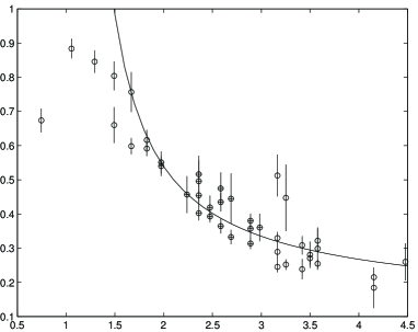
By fitting the data to (3.2) we obtain two estimates for (,), namely (,) and (,), with comparable values for . The momentum range for the fit corresponds to GeV. We take the first set of values as our best estimate of the parameters as the corresponding value of is close to what is obtained from a “pure” two-loop fit, i.e. is stable with respect to the introduction of power corrections. This choice will be supported also by independent considerations at the three-loop level. In summary, a two-loop description with power corrections based on (3.2) fits well the data in a consistent momentum range. Our best fit is shown in Figure 1.

3.3 Three-loop analysis
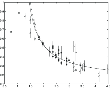
A major obstacle for a three-loop analysis is our ignorance of the first non-universal coefficient of the perturbative -function. In order to gain insight, we perform a two-parameter fit to the “pure” three-loop formula, taking and the unknown coefficient as the fitting parameters. We call the fit estimate for . We obtain , , with (see dashed curve in Fig. 2). The momentum range where we obtain the best description of the data is GeV. Our result for provides (via perturbative matching) an estimate for which is in very good agreement with the estimate in [10], which was obtained from the computation of the parameter in a completely different scheme. Although our estimate depends on the extra parameter , the agreement between the two results is remarkable.
So far, the success of the “pure” three-loop fit suggests that the power term in the two-loop formula merely provides an effective description of three-loop effects. However, it turns out that there is room for a power correction even at the three-loop level. To see this, we consider a three-loop formula with a power correction:
| (4) |

where and is again to be determined from a fit. Fitting the data to (3.3), we obtain , and , with , in a momentum range (see Fig. 2). We note that the value for is fully consistent with the previous determination from the “pure” three-loop description. The value for is also reasonably stable with respect to the previous determination. By comparing results from fits to (3.2) and (3.3), it emerges that
| (5) |
In other words, the power terms providing the best fit to (3.2) and (3.3) are numerically the same, so that there seems to be no interplay between the indetermination connected to the perturbative terms and the power correction term, within the precision of our data. We take this fact as an indication that a description in terms of power corrections is still relevant at the three-loop level. Notice that the numerical value of the power correction is comparable to the standard estimate for the string tension.
One could object that at the two-loop level we had chosen between two sets of values for (,), and that our choice is crucial for the validity of (5). An a posteriori justification for our choice is obtained from the following test: we plot a few values for as generated by the “pure” three-loop formula for and . Then, by fitting such points to the “pure” two-loop formula, one gets , i.e. the value for which (5) holds. Again, the above test seems to confirm that perturbative and non-perturbative contributions do not mix in our formulae when upgrading from a two-loop to a three-loop description, thus suggesting that a genuine correction is present in the data.
4 CONCLUSIONS
We have discussed an exploratory investigation of power corrections in the running QCD coupling by comparing non-perturbative lattice results with theoretical models. Some evidence was found for corrections, whose size would be consistent with what is suggested by simple arguments from the static potential.
Our results need to be further tested by the analysis of a larger data set and by a study of the dependence of the fit coefficient on the ultraviolet and infrared lattice cutoff. A very delicate issue is the assessment of the scheme dependendence of our results. In particular, we note that the definition of the coupling that we adopted is a priori gauge-dependent. This point will be the focus of our future work.
5 ACKNOWLEDGEMENTS
We thank B. Alles, H. Panagopoulos and D. G. Richards for allowing us to use data files containing the results of Ref. [12]. C. Parrinello acknowledges the support of PPARC through an Advanced Fellowship. C. Pittori thanks J. Cugnon and the “Institut de Physique de l’Université de Liège au Sart Tilman” and acknowledges the partial support of IISN. We thank C. Michael for stimulating discussions.
References
- [1] R. Akhoury and V.I. Zakharov, hep-ph/9705318.
- [2] G.Grunberg, hep-ph/9705290, hep-ph/9705460.
- [3] G Burgio, F. Di Renzo, G. Marchesini and E. Onofri, Phys. Lett. 422B (1998) 219.
- [4] G. Altarelli, et al, Zeit. Phys. C68 (1995) 257.
- [5] G.P. Lepage and P. Mackenzie, Nucl. Phys. Proc. Suppl. 20 (1991) 173.
- [6] Yu.L. Dokshitzer, G. Marchesini and B.R. Webber, Nucl. Phys. B469 (1996) 93
- [7] S.J. Brodsky, G.P. Lepage and P.B. Mackenzie, Phys. Rev. D 28 (1983) 228.
- [8] R. Akhoury and V.I. Zakharov, hep-ph/9710487.
- [9] See, for example, P. Redmond, Phys. Rev. D 112 (1958) 1404.
- [10] S. Capitani et al, Nucl. Phys. Proc. Suppl. 63 (1998) 153.
- [11] C. Parrinello, Phys. Rev. D50 (1994) 4247.
- [12] B. Allés et al, Nucl. Phys. B502 (1997) 325