HUPD-9719
hep-ph/9711260
QCD Higher Order Corrections
to at Small
***Talk presented by J. Kodaira. To appear in:
Proceedings of the Workshop on Deep Inelastic Scattering
off Polarized Targets: Theory Meets Experiment,
DESY Zeuthen, September 1-5, 1997.
Yuichiro KIYO, Jiro KODAIRA and Hiroshi TOCHIMURA
Dept. of Physics, Hiroshima University Higashi-Hiroshima
739, JAPAN
Abstract
The small behavior of the flavor non-singlet structure function is analysed numerically by taking into account the all-order resummation of terms. We include a part of the next-to-leading logarithmic corrections coming from the resummed “coefficient function” which are not considered in the literatures to respect the factorization scheme independence. The resummed coefficient function turns out to give unexpectedly large suppression effects over the experimentally accessible range of and . This fact implies that the higher order logarithmic corrections are very important for in the small region.
1 Introduction
The behavior of the structure function in the small Bjorken region has recently received much attention of the physicists [1]. This region corresponds to the so-called Regge limit. So we naively expect that the soft physics (Regge theory) may explain the small behavior of the structure function. However the steep rise of the structure function in this region observed by the HERA experiments contradicts with this naive expectation. The physics at small is now one of the most interesting subjects and many people believe that this problem could be handled in the context of the QCD perturbation theory [2].
In the case of the polarized structure function , we have not yet had data at very small [3]. However it is very important and desirable to know the small behavior of in the light of the Bjorken and Ellis-Jaffe sum rules. The naive Regge theory tells us,
at small and and this implies a “flat” input parton density. Although the recent detailed analyses [4] of the existing data in the DGLAP approach do not necessarily require an input function which contradicts with the naive Regge prediction, it is inevitable to take into account the effects from the corrections, which appear in the perturbative calculations, to get more precise predictions on the small behavior of [5].
Bartels, Ermolaev and Ryskin [6] have given the resummed expression for the structure function by using the Infra-Red Evolution Equation and confirmed the old result by Kirschner and Lipatov [7]. They claim that the resummation effects may be very important. On the other hand, the numerical analysis by Blümlein and Vogt [8] shows that there are no significant contributions from the resummation of the leading logarithmic (LL) corrections in the HERA kinematical region ( ). This controversial aspect might come from the fact that the resummed “coefficient function” is considered in Ref. [6] but not in Ref. [8]. Blümlein and Vogt did not include the resummed coefficient function because it falls in the next-to-leading logarithmic (NLL) corrections and depends on the factorization scheme adopted. It is also to be noted that the evolution, in general, strongly depends on the input parton densities. If one chooses a steep input function, the perturbative contribution will be completely washed away. So it will be interesting to see also the sensitivity of the results to the choice of the input densities.
In this report, we discuss the numerical impact of the all-order resummation on the small behavior of (non-singlet part). We consider two different input densities: one is flat corresponding to the naive Regge prediction and the other is steep in the small region. The coefficient function can not be included consistently at present since the anomalous dimension has been calculated only at the LL order. However we consider the effects of the coefficient function because we could firstly clarify the above controversial aspect and secondly get some idea about the magnitude of the NLL order corrections in the resummation approach. Details of the calculations may be found in ref. [9].
2 Resummation of terms
The flavor non-singlet part of in the moment space is given by,
where
and () is the flavor non-singlet combination of the polarized parton densities (the coefficient function). is the average of quark’s electric charge. The DGLAP equation reads,
| (1) |
Here the anomalous dimension is the moment of the “splitting” function.
The coefficient function and the anomalous dimension may be expanded in the powers of ,
where . The singular behaviors of these functions as appear as the pole singularities at . When is finite, it may be enough to compute them to the fixed-order of perturbation. In the small region, however, the fixed-order calculation becomes questionable since there appear type corrections. If these terms compensate the smallness of the coupling constant , we must resum the perturbative series to the all orders to get a reliable prediction. The explicit next-to-leading order (NLO) calculations [10] [11] in the scheme show a strong singularity at ,
| (2) |
These strong singularities (double logarithmic corrections) will persist to all orders of perturbative series. Indeed, at the -th loop, the anomalous dimension and the coefficient function are expected to behave as,
| (3) |
Our task is to resum these terms to all-orders in the perturbative expansion.
The resummation of singularities for has been done in Refs. [6] [7]. The result for the “parton (quark) ” target with the fixed †††In the genuine LL approximation, the strong coupling constant should be taken as a fixed parameter. reads,
where is an arbitrary mass scale which regularizes the infrared and/or mass singularities. From this expression we could identify the resummed anomalous dimension and the coefficient function to be,
| (4) | |||||
| (5) |
Here is given by,
with
is the parabolic cylinder function.
Now it will be instructive to re-expand Eqs.(4,5) in terms of to see whether these formulae sum up the most singular terms of the perturbative series. The expressions expanded up to read,
| (6) | |||||
| (7) | |||||
These results coincide with the previous expectation of Eq.(3). Furthermore one can easily see that the resummed expressions Eqs.(4,5) reproduce the known NLO results Eqs.(2) in the scheme ‡‡‡This statement seems questionable beyond the NLO as stressed by J. Blümlein.. Therefore, it is quite plausible that Eqs.(4,5) correctly sum up the “leading” singularities to all orders.
Here a comment is in order concerning the scheme dependence. The anomalous dimension and the coefficient function individually depend on the factorization scheme. (Unfortunately we do not have by now any appropriate factorization theorems to the problem discussed in this report.) In particular, the resummed “coefficient function” does not have any physical meaning until the scheme dependent part of the anomalous dimension is calculated in the same scheme. To clarify this issue, let us write the above results in the form which corresponds to the so-called DIS scheme. The parton densities and anomalous dimension in the DIS scheme are obtained by making the transformations,
Using the resummed and Eqs.(6,7), we get the resummed part of the anomalous dimension in the DIS scheme,
| (8) |
where the second terms come from the resummed coefficient function and are numerical numbers independent of . The above equation tells us that the resummed coefficient function belongs to the NLL order corrections in the context of the resummation approach. Then, one must include the NLL order anomalous dimension, which has not yet been available, to see the NLL effects.
3 Numerical Analysis
Now we come to the numerical analyses to show how the final results are sensitive to the choice of the input parton densities. In conjunction with the claim in Ref. [6], we also consider the effects from the resummed coefficient function with the hope that the inclusion of it could shed some light on the size of the NLL corrections.
Our starting point is the expression,
| (9) |
The anomalous dimension which includes the resummation of terms is organized as follows,
| (10) |
where and are respectively the exact anomalous dimension and coefficient function at the one and two-loop fixed order perturbation theory. () is the resummed anomalous dimension Eq.(6) (Eq.(7)) with () terms being subtracted.
It is to be noted here that the anomalous dimension at should vanish due to the conservation of the (non-singlet) axial vector current. The perturbation theory guarantees this symmetry order by order in the expansion. However, the resummation of the leading singularities in does not respect this symmetry. Therefore, we need to restore this symmetry “by hand”. Our choice is [8],
Of course, this is not a unique prescription §§§Our final conclusion remains the same qualitatively if we choose other prescription.. We have used the technique in Ref. [12] to perform the Mellin inversion Eq.(9).
We choose the starting value of the evolution to be . We calculate the evolution for two types of the input densities A and B: A is a function which is flat at small (), and B is slightly steep (). The explicit parametrization we use is [4],
where is a normalization factor such that and () in accordance with the Bjorken sum rule. A and B correspond to the following values of parameters,
We put the flavor number and .
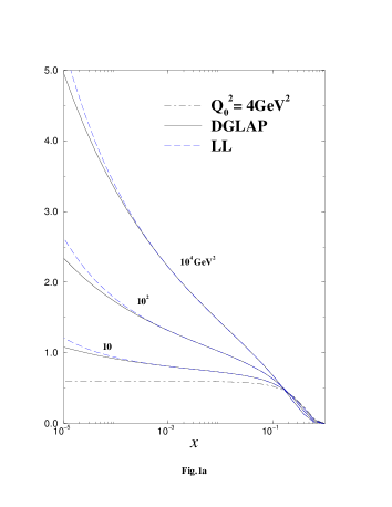
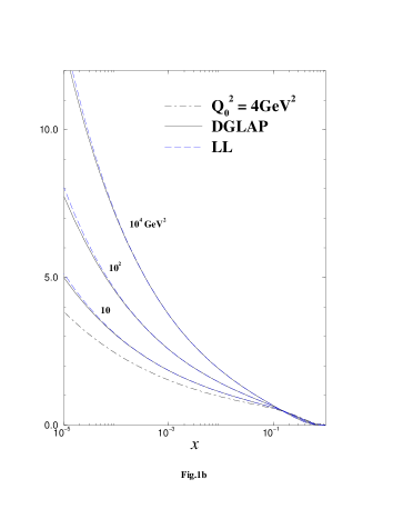
First we estimate the case which includes only the LL correction . The evolution kernel in this case is obtained by dropping in Eq.(10). Fig.1a (1b) shows the LL results (dashed curves) after evolving to from the A (B) input density (dot-dashed line). The solid curves are the predictions of the NLO-DGLAP evolution. These results show a tiny enhancement compared with the NLO-DGLAP analysis and are consistent with those in Ref. [8] The enhancement is, as expected, bigger when the input density is flatter. However any significant differences are not seen between the results from different input densities.
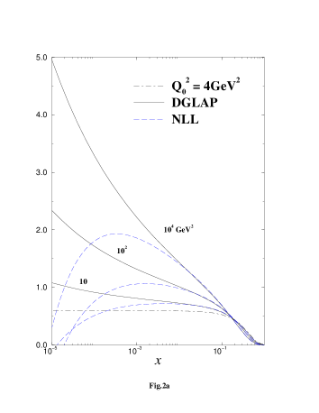
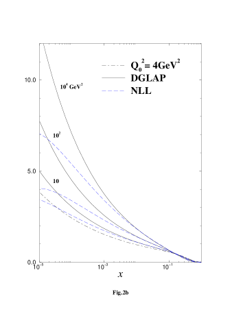
Next, we include the NLL corrections from the resummed “coefficient function”. We show the results in Fig.2 by the dashed curves. The results are rather surprising. The inclusion of the coefficient function leads to a strong suppression on the evolution of the structure function at small . Since the effects from the coefficient function fall in the NLL level, the LL terms are expected to (should) dominate at the small . However our results imply that the LL approximation is not sensible in the small region we are interested in. As the resummed coefficient function is only a part of the NLL correction, we can not present a definite conclusion on the (full) NLL correction. But it is obvious that the NLL correction is very important in the experimentally accessible region of .
 |
 |
 |
 |
4 Discussion
In the previous section, we have shown that although the LL resummed effect is very small in the experimentally accessible region of , a part of the NLL resummed contribution from the coefficient function drastically changes the predictions. To understand these numerical results, it will be helpful to remember the perturbative expansion of the resummed results Eqs.(6,7). Using the explicit values , we obtain for the anomalous dimension in the DIS scheme Eq.(8),
Here note that: (1) the perturbative coefficients of the LL terms (the first part of Eq.(4)) are negative and those of the higher orders are rather small number. This implies that the LL corrections push up the structure function compared to the fixed-order DGLAP evolution, but the deviations are expected to be small. (2) the perturbative ones from the NLL terms (the second part of Eq.(4)), however, are positive and somehow large compared with those of the LL terms. This positivity of the NLL terms has the effect of decreasing the structure function. This fact that the coefficients with both sign appear in the anomalous dimension should be contrasted with the case of the unpolarized structure function [2].
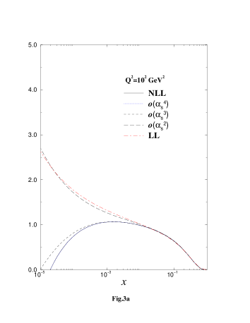
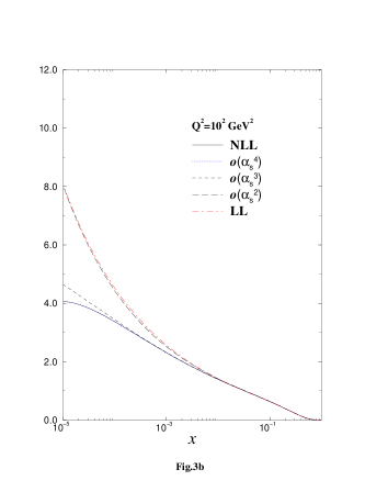
Now it might be also helpful to assume that the saddle-point dominates the Mellin inversion Eq.(9). We have numerically estimated the approximate position of the saddle-point and found that the saddle-point stays around in the region of to . By looking at the explicit values of the coefficients in Eq.(4), the position of the saddle-point seems to suggest that the NLL terms can not be neglected. Since the coefficients from the higher order terms are not so large numerically, it is also expected that the terms which lead to sizable effects on the evolution may be only first few terms in the perturbative series in the region of we are interested in. We have checked that the inclusion of the first few terms in Eq.(4) already reproduces the results of section 3. Fig.3a (3b) shows the numerical results of the contribution from each terms of the NLL corrections in Eq.(4) at with the A (B) type input density. The solid (dot-dashed) line corresponds to the NLL (LL) result. The long-dashed, dashed and dotted lines correspond respectively to the case in which the terms up to the order , , , are kept in the NLL contributions. One can see that the dotted line already coincides with the full NLL (solid) line. These considerations could help us to understand why the NLL corrections turns out to give large effects.
 |
 |
The final discussion concerns the convergence issue of the perturbative series. As discussed in Refs. [13], one must be careful when applying the perturbative approach to small evolution. So according to Refs. [13], we have tried to solve the evolution in space with first several terms of the perturbative expansion being kept and what we found is that the conclusion does not change. The numerical results remain essentially the same.
In summary, we have performed numerical studies for the flavor non-singlet at small by incorporating the all-order resummed anomalous dimension and a part of the NLL corrections from the resummed coefficient function. Including only the resummed coefficient part is not theoretically consistent, and so one should take into account also the anomalous dimension at the NLL level. However, our results suggest that the LL analysis is unstable, in the sense that a large suppression effect comes from the resummed coefficient function which should be NLL correction. We need a full NLL analysis to make a definite conclusion.
J.K. would like to thank the organisers of this workshop for their hospitality. This work was supported in part by the Monbusho Grant-in-Aid Scientific Research No. A (1) 08304024, No. C (1) 09640364 and the Monbusho International Scientific Research No. 08044089.
References
- [1] See e.g. J. Blümlein, S. Riemersma and A. Vogt, Preprint DESY 96-131 / WUE-ITP-96-016 hep-ph/9608470; hep-ph/9610427 and references therein.
- [2] L. N. Lipatov, Sov. J. Nucl. Phys. 23 (1976) 338; E. A. Kuraev, L. N. Lipatov and V. S. Fadin, Sov. Phys. JETP 45 (1977) 199; Ya. Balitskii and L. N. Lipatov, Sov. J. Nucl. Phys. 28 (1978) 822; S. Catani and F. Hautmann, Nucl. Phys. B427 (1994) 475; S. Catani, Z. Phys. C70 (1996) 263 and references therein.
- [3] R. Windmolders, Talk at this Workshop; C. Young, Talk at this Workshop; D. Hasch, Talk at this Workshop.
- [4] M. Stratmann, Talk at this Workshop. S. Forte, Talk at this Workshop.
- [5] A. Vogt, Talk at this Workshop; R. Kirschner, Talk at this Workshop.
- [6] J. Bartels, B. I. Ermolaev and M. G. Ryskin, Z. Phys. C70 (1996) 273; ibid. C72 (1997) 627.
- [7] R. Kirschner and L. N. Lipatov, Nucl. Phys. B213 (1983) 122.
- [8] J. Blümlein and A. Vogt ,Phys. Lett. B370 (1996) 149 ; Acta.Phys.Polonica B27 (1996) 1309; J. Blümlein, S. Riemersma and A. Vogt, hep-ph/9608470
- [9] Y. Kiyo, J. Kodaira and H. Tochimura, Z. Phys. C74 (1997) 631.
- [10] J. Kodaira, S. Matsuda, T. Muta, K. Sasaki and T. Uematsu, Phys. Rev. D20 (1979) 627; J. Kodaira, S. Matsuda, K. Sasaki and T. Uematsu, Nucl. Phys. B159 (1979) 99.
- [11] R. Mertig and W. L. van Neerven, Z. Phys. C70 (1996) 637 and references therein.
- [12] M. Glück, E. Reya and A. Vogt, Z. Phys. C48 (1990) 471; D. Graudenz, M. Hampel, A. Vogt and Ch. Berger, Z. Phys. C70 (1996) 70.
- [13] R. D. Ball and S. Forte, Phys. Lett. B351 (1995) 313; J. R. Forshaw, R. G. Roberts and R. S. Thorne, Phys. Lett. B356 (1995) 79.