CPT-94/P.3098

Southampton Preprint SHEP 94/95-07

Weak Decays of $B$ Mesons and Lattice QCD

Laurent LELLOUCH
Centre de Physique Théorique

CNRS–Luminy, Case 907

F-13288 Marseille Cedex 9, France

After a pedagogical introduction to the calculation of weak matrix elements on the lattice, I review some of the lattice’s most recent predictions concerning the weak decays of $B$-mesons. Amongst the topics covered are the determinations of the leptonic decay constant $f_{B}$, of the form factors relevant for semi-leptonic $B\to D(D^{*})\ell\bar{\nu}$ decays and of the hadronic matrix element which describes the rare decay $B\to K^{*}\gamma$. Emphasis is placed on the results of the UKQCD Collaboration. Corrections to the heavy-quark limit are discussed extensively.

1 Introduction

Weak decays of hadrons are a very rich source of information about the Standard Model. Not only do they enable us to determine from experiment the parameters which are associated with the flavor sector of the Standard Model but they also provide a rich testing ground for understanding the non-perturbative dynamics of the strong interaction. These two aspects of hadronic, weak decays are in fact inseparable. To be more specific, the Standard Model prediction for the rate of such a decay follows the pattern

$$\mbox{rate}=\left\{\begin{array}[]{l}\mbox{kinematical}\\ \mbox{factors}\\ \end{array}\right\}\left\{\begin{array}[]{l}\mbox{Non-Perturbative}\\ \mbox{QCD factor}\\ \end{array}\right\}\left\{\begin{array}[]{l}\mbox{CKM}\\ \mbox{factor}\\ \end{array}\right\}$$ (1)

from which it is clear that in order to extract the Cabibbo-Kobayashi-Maskawa (CKM) factor from an experimental measurement of the rate, one has to understand or at least calculate the non-perturbative QCD factor. The lattice formulation of QCD, together with large scale numerical simulations, provides a natural framework for evaluating this factor. It is in fact the only systematic, first-principle approach we know for quantifying non-perturbative, strong-interaction dynamics with the QCD lagrangian as a starting point. This should not be taken to mean that it is only approach or even the most efficient approach, as QCD sum-rules, low energy effective theories and quark models have provided many important and reliable results throughout the years.

The latest chapter in the story of hadronic weak decays concerns hadrons containing a $b$-quark. The decays of these hadrons are interesting phenomenologically because their study will enable us to determine the least well know column of the CKM matrix. They are also interesting theoretically because they provide a ground for testing heavy-quark symmetry. Heavy-quark symmetry is a symmetry of QCD that arises in the limit that the mass of the heavy quark is much larger than the QCD scale $\Lambda_{\rm QCD}$. In that limit one finds that the dynamics of the light quarks and gluons coupled to the heavy quark become independent of the heavy quark’s flavor and spin. To the extent, then, that $\Lambda_{\rm QCD}$ is negligible compared to the masses of the charm and beauty quarks, QCD exhibits a new $SU(4)_{spin\times flavor}$ symmetry which acts on the multiplet $(c\uparrow,c\downarrow,b\uparrow,b\downarrow)$[1, 2]. This symmetry tremendously simplifies the description of the decays of hadrons containing a heavy quark. It has in fact been incorporated into the framework of an effective theory[3] known as Heavy Quark Effective Theory (HQET). This makes it possible to systematically calculate corrections to the symmetry limit order by order in inverse powers of the heavy-quark masses much in the same way that Chiral Lagrangians enables one to calculate corrections to the predictions of the spontaneously broken chiral symmetry of QCD in the light quark sector. I would like to emphasize, at this point, that the lattice is supremely well suited for studying the range of applicability of heavy-quark symmetry, for the masses of the heavy quarks are free parameters in lattice calculations and the dependence of results on heavy-quark mass can be studied in detail.

In the present article I will review some of the latest results of lattice calculations of weak matrix elements of beautiful hadrons. I will concentrate mainly on the results of the UKQCD Collaboration because this article is not meant to be thorough and systematic review of the subject but rather an introduction to the methods, possibilities and limitations of this rapidly growing field. In Section 2 I will provide a introduction to lattice calculations of weak matrix elements. For a more complete review, see the lectures of R. Gupta in the present volume or the reviews in [5]. For reviews about $b$-physics on the lattice, see Ref.[6]. In Section 3, I will present results for the $B$-meson decay constant, $f_{B}$, and will describe what these results teach us about heavy-quark symmetry. I will then turn to the subject of semi-leptonic $B_{(s)}\to D_{(s)}$ and $B_{(s)}\to D^{*}_{(s)}$ decays in Section 4. I will present determinations of the Isgur-Wise functions $\xi_{u,d}$ and $\xi_{s}$ which parametrize the strong interaction effects to leading order in heavy-quark mass in these decays. I will show how the function $\xi_{u,d}$ can be used to extract the CKM matrix-element $V_{cb}$ from an experimental measurement of the differential decay rate for $B\to D^{*}\ell\nu$ decays. I will also present many tests of the heavy-quark symmetry which involve comparing $B\to D$ and $B\to D^{*}$ decays for many different values of the $b$ and $c$ quark masses. Section 5 will be dedicated to a lattice evaluation of the rate for the rare process $B\to K^{*}\gamma$. This process occurs through a flavor-changing-neutral-current, penguin diagram and was first observed in 1993 by the CLEO collaboration[7]. I will end the article in Section 6 with a summary and conclusions.

2 Matrix Element Calculations on the Lattice

2.1 What We Calculate

To obtain matrix elements in lattice calculations we compute expectation values of products of gluon and quark fields at different spacetime points. We do so using the path integral formulation of QCD in euclidean spacetime. Thus, given a product ${\cal O}(x_{1},\cdots,x_{n})$ of quark and gluon fields, we compute $n$-point functions:

$$\langle{\cal O}(x_{1},\cdots,x_{n})\rangle=\frac{1}{Z}\int dA_{\mu}d\bar{\psi}d\psi\ {\rm e}^{-S_{QCD}}{\cal O}(x_{1},\cdots,x_{n})\ ,$$ (2)

where $S_{QCD}$ is the QCD action and

$$Z=\int dA_{\mu}d\bar{\psi}d\psi\ {\rm e}^{-S_{QCD}}\ .$$ (3)

The simplest example of an $n$-point function is the 2-point function. To determine the decay constant of a $B$-meson, for instance, we would evaluate the 2-point function

$$\sum_{{\bf x}}\langle\bar{q}\gamma^{\mu}\gamma^{5}b({\bf x},t)\ \bar{b}\gamma^{5}q(0)\rangle\ ,$$ (4)

where $q$ is a light-quark field and the sum over ${\bf x}$ ensures that the meson is at rest. If we insert a complete set of states between the two operators in Eq. (4) we find that this correlator decays exponentially in time in the limit of large $t$. The rate of the decay is governed by the mass of ground state and its amplitude is proportional to the weak matrix element, $\langle 0|\bar{q}\gamma^{\mu}\gamma^{5}b(0)|B\rangle$, we are after:

$$\sum_{{\bf x}}\langle\bar{q}\gamma^{\mu}\gamma^{5}b({\bf x},t)\ \bar{b}\gamma^{5}q(0)\rangle\buildrel\;\;t\to\infty\;\;\over{\longrightarrow}\frac{\langle 0|\bar{q}\gamma^{\mu}\gamma^{5}b(0)|B\rangle\,\langle B|\bar{b}\gamma^{5}q(0)|0\rangle}{2m_{B}}\ {\rm e}^{-m_{B}t}\ .$$ (5)

The next level of complexity is the 3-point function. The matrix element $\langle D({\bf p}^{\prime})|\bar{c}\gamma^{\mu}b(0)|B({\bf p})\rangle$, for instance, is obtained from the 3-point function

$$\sum_{{\bf x},{\bf y}}{\rm e}^{-i{\bf p}^{\prime}\cdot{\bf y}-i{\bf q}\cdot{\bf x}}\langle\bar{c}\gamma^{5}q({\bf y},t_{f})\,\bar{c}\gamma^{\mu}b({\bf x},t)\,\bar{b}\gamma^{\mu}q(0)\rangle$$ (6)

where ${\bf q}={\bf p}-{\bf p}^{\prime}$. In the limit that $t,\,t_{f}-t\to\infty$, this 3-point function reduces to

$$\frac{\langle 0|\bar{q}\gamma^{5}b(0)|D({\bf p}^{\prime})\rangle\,\langle D({\bf p}^{\prime})|\bar{c}\gamma^{\mu}b(0)|B({\bf p})\rangle\,\langle B({\bf p})|\bar{b}\gamma^{5}q(0)|0\rangle}{4E_{D}E_{B}}\ {\rm e}^{-E_{B}t-E_{D}(t_{f}-t)}\ ,$$ (7)

where $E_{B}$ and $E_{D}$ are the energies of the $B$ and $D$ mesons, respectively.

2.2 How We Calculate

The first step in evaluating the path integral of Eq. (2) is to approximate spacetime by a finite, hypercubic lattice. Quark fields are then placed on the sites of this lattice and the gluon fields on the links between these sites. This reduces the integral over gluon and quark fields to an integral over a finite number of degrees of freedom which makes it amenable to numerical methods. It is important to note, at this point, that to preserve gauge invariance on a discretized spacetime one works with elements of the group–the link variables $U_{\mu}(x)=e^{iagA_{\mu}(x)}$–instead of with the gauge fields $A_{\mu}(x)$ (see Ref.[8], for example). This means, for instance, that the integrals over gauge fields in Eqs. (2) and (3) are actually integrals over the compact link variables $U_{\mu}(x)$.

As a first step in the evaluation of this lattice path integral, we generate a number $N$ of gluon configurations by a Monte-Carlo simulation[9] with the probability distribution

$${\cal P}\equiv\frac{{\rm e}^{-S_{gluon}}\times{\rm det}(D\hskip-7.68236pt/+M)}{Z}\ ,$$ (8)

where $S_{gluon}$ is a discretized gluon action[8], $D_{\mu}$ a discretized $SU(3)$ covariant derivative in the fundamental representation and $M$, the quark-mass matrix. Then, for example, to obtain the propagator of a $B$-meson,

$$\langle\bar{u}\gamma^{5}b(x)\,\bar{b}\gamma^{5}u(0)\rangle\ ,$$ (9)

we use Wick’s theorem to reduce the quark bilinears in Eq. (9) to a product of quark propagators and do so for each one of the $N$ gluon backgrounds. The meson propagator then becomes the following average of a product of quark propagators and Dirac matrices over gluon backgrounds,

$$\langle\bar{u}\gamma^{5}b(x)\,\bar{b}\gamma^{5}u(0)\rangle=\frac{1}{N}\sum_{U_{\mu}}{\rm Tr}\left(\gamma^{5}S_{b}(0,x;U_{\mu})\gamma^{5}S_{u}(x,0;U_{\mu})\right)\ ,$$ (10)

which can be evaluated numerically once the propagators, $S_{b(u)}(0,x;U_{\mu})$, for the $b$ and $u$ quarks in the gluon background $U_{\mu}$ have been calculated using matrix inversion algorithms such as the conjugate gradient algorithm[10].

2.3 Limitations and Sources of Errors

Even though the numerical evaluation of the path integral of Eq. (2) described in Section 2.2 is an ab initio calculation starting with the QCD lagrangian, the final results have errors which are due to the approximations that have to be made. These errors can be classified into two broad categories. There are statistical errors which arise because we use statistical methods to evaluate the path integral and systematic errors which arise because we approximate spacetime by a finite lattice of points and because we usually have to neglect the contributions of fermion loops. One may wonder, at this point, what advantage the lattice has over other means of evaluating hadronic properties. The difference lies in that the errors made in a lattice calculation can be reduced systematically by increasing the number of configurations and the physical volume of the lattice, by decreasing the lattice spacing or by designing lattice actions which converge to the continuum limit more rapidly.

2.3.1 Statistical Errors

Statistical errors arise because we approximate the integral over gauge fields, which is an integral over an infinite number of configurations, by a sum over a finite number, $N$, of configurations. According to the central limit theorem, the error made on $n$-point functions is proportional to $1/\sqrt{N}$ in the limit of large $N$, so that statistical errors decrease as the number of configurations increases. Typical values of $N$ in QCD calculations are on the order of 100 and the corresponding errors are on the order of a few percent for many quantities. We evaluate these errors using standard statistical methods such as the bootstrap or jacknife method[11]. These methods enable us to approximately determine the distribution of results we would find were we to repeat our $N$-configuration calculation many times. The statistical error we quote on our result is chosen to include to the central 68% of this distribution.

2.3.2 Discretization Errors

Discretization errors are due to the fact that we approximate spacetime by a discrete lattice of points. To see how these errors arise, consider the symmetric lattice derivative of a function, $f$, of spacetime in the limit that the lattice spacing $a$ is taken to zero:

$$\frac{f(x+a\hat{\mu})-f(x-a\hat{\mu})}{2a}\buildrel\;\;a\to 0\;\;\over{\longrightarrow}\partial_{\mu}f(x)+{\cal O}\left(a^{2}\right)\ ,$$ (11)

where $\hat{\mu}$ is a unit vector in the $\mu$-direction. It is clear from Eq. (11) that approximating the derivative of $f$ by a finite difference introduces an error of order $a^{2}$. Before exploring these discretization errors in more detail, though, I shall first describe how we determine the lattice spacing $a$ from our simulations.

Setting the Scale

As you well know, the bare coupling constant $g(a)$ is related to the cutoff $a$ through dimensional transmutation. Before performing our simulation, however, we only know what this relation is through perturbation theory up to some finite order in $g(a)$. So it is preferable not to fix both quantities from the start. What we do is pick a value for the bare coupling, $\beta=2N_{c}/g^{2}(a)$, and rewrite the QCD lagrangian in terms of dimensionless quantities, measured in units of the lattice spacing $a$. All explicit dependence on $a$ then disappears from the problem and $a$ need not be fixed before performing the simulation. Once the simulation has been performed, however, $a$ must be determined so that physical dimensions may be restored. To do this, we pick a dimensionful, physical quantity such as the string tension $\sigma$. The lattice spacing is then the ratio of the experimental value, $\sigma^{\rm expt}$, to the dimensionless quantity, $\sigma^{\rm latt.}$, that our simulation yields, raised to the appropriate power:

$$a^{-1}=\sqrt{\frac{\sigma^{\rm expt}}{\sigma^{\rm latt}}}\ .$$ (12)

To set the scale any dimensionful quantity will do though different quantities will lead to more or less accurate determinations of the lattice spacing. In Table 1, I show the values for $a^{-1}$ that our collaboration obtains from various physical quantities. All of these quantities should, in principle, yield the same lattice spacing assuming, of course, that QCD is correct. The reason why the values in Table 1 do not agree within the quoted statistical errors is because we also make systematic errors. In fact, the range of values that we obtain for $a^{-1}$ is a good indication of the size of the systematic errors we make.

Physical Quantity	$a^{-1}$ (${\,\rm GeV}$)
$\sqrt{\sigma}$ (string tension)	2.73(5)
$m_{\rho}$ (mass of the $\rho$)	$2.7\raisebox{0.80002pt}{\scriptsize{$\;\begin{array}[]{@{}l@{}}\makebox[15.0pt][c]{$+$}\makebox[3.85002pt][r]{1}\\[-0.83997pt] \makebox[15.0pt][c]{$-$}\makebox[3.85002pt][r]{1}\end{array}$}}$
$m_{N}$ (mass of the nucleon)	$3.0\raisebox{0.80002pt}{\scriptsize{$\;\begin{array}[]{@{}l@{}}\makebox[15.0pt][c]{$+$}\makebox[3.85002pt][r]{2}\\[-0.83997pt] \makebox[15.0pt][c]{$-$}\makebox[3.85002pt][r]{3}\end{array}$}}$
$m_{\Delta}$ (mass of the $\Delta$)	$2.5\raisebox{0.80002pt}{\scriptsize{$\;\begin{array}[]{@{}l@{}}\makebox[15.0pt][c]{$+$}\makebox[3.85002pt][r]{2}\\[-0.83997pt] \makebox[15.0pt][c]{$-$}\makebox[3.85002pt][r]{2}\end{array}$}}$

Table 1: Values of the inverse lattice spacing, $a^{-1}$, for UKQCD’s $\beta=6.2$, $24^{3}\times 48$ lattice as obtained from different physical quantities [12]. Ratios of these different values indicate how well the corresponding ratio of physical quantities is predicted by the simulation. $a^{-1}(m_{\rho})/a^{-1}(m_{N})$, for instance, indicates that the ratio $m_{N}/m_{\rho}$ comes out 10% low in our simulation but with errors large enough to make it consistent with experiment.

Having established how one determines the lattice spacing, we return to the discussion of discretization errors and how to reduce them. The reason why these errors are particularly important in simulations of hadrons containing a heavy quark is because these quarks have very short compton wavelengths: an accurate description of their quantum propagation appears to require a very fine lattice. There are in fact many different ways to describe heavy quarks on a lattice. These different approaches fall into two broad categories. In the first category, the quark action used is simply a discretization of the full continuum quark action. In the second, that of effective theories, this discretized action is further expanded in inverse powers of the heavy-quark mass as well as in powers of the heavy quark’s velocity if the heavy quark is non-relativistic.

The Wilson Action

One of the standard discretizations of the continuum quark action is the Wilson action[8]:

$$S^{W}=a^{4}\ \sum_{x} \Biggl{\{}-\frac{1}{2a}\sum_{\mu}\left[\bar{q}(x)(r-\gamma_{\mu})U_{\mu}(x)q(x+a\hat{\mu})+\bar{q}(x+a\hat{\mu})(r+\gamma_{\mu})U_{\mu}^{\dagger}(x)q(x)\right]$$ (13)

$$+\bar{q}(x)\left(m_{o}+\frac{4r}{a}\right)q(x)\Biggr{\}}\ ,$$

where $r$ is a number (typically taken to be 1) known as the Wilson parameter. In the naive continuum limit, this action reduces to

$$S^{W}\buildrel\;\;a\to 0\;\;\over{\longrightarrow}\int\bar{q}\left(D\hskip-7.68236pt/+m_{o}\right)q-\frac{ar}{2}\int\bar{q}D^{2}q+{\cal O}\left(a^{2}\right)\ .$$ (14)

Because of the ${\cal O}\left(a\right)$ term, we expect the leading discretization errors, in a simulation of a hadron containing a heavy quark, to be on the order of $am_{Q}$, where $m_{Q}$ is the mass of the heavy quark. For these errors to remain under control, we must require $am_{Q}\ll 1$. Since typical values of the inverse lattice spacing are on the order of $3{\,\rm GeV}$, the $b$ quark, which has a mass of about $4.5{\,\rm GeV}$, cannot be simulated directly. Thus, the strategy used to obtain properties of $b$-hadrons with the Wilson action is to calculate these properties for a collection hadrons whose heavy quarks have a mass in the range of the charm quark mass and then to extrapolate these properties in heavy-quark mass to $m_{b}$, using HQET as a guide. But even for the charm quark, we expect large discretization errors as $am_{c}\sim 0.4$ for a typical value of the lattice spacing. So if the Wilson action is to be used, one has to find a way to reduce these discretization errors.

The brute force approach to reducing discretization errors is to increase the number of lattice sites and reduce the lattice spacing. This requires ever faster computers. The second type of approach is to design lattice theories which converge faster to the continuum limit. It is to this second approach we now turn.

Improving the Wilson Action: Normalization of Quark Fields

The impetus for the improvement that I am going to describe comes from an analysis of the free-fermion propagator on the lattice. One finds, using the action given in Eq. (13), that this propagator is given, at zero momentum, by

$$\sum_{{\bf x}}S^{W}(x,0)={\rm e}^{-am}\ \left[\frac{1+\gamma_{o}}{2}\,{\rm e}^{-mt}\right]\ ,$$ (15)

where the term in brackets is the continuum, free propagator for a fermion of mass

$$am={\rm ln}\left(1+am_{o}\right)\ .$$ (16)

In the limit that $am_{o}$ vanishes, the lattice propagator in Eq. (15) reduces to the continuum propagator for a fermion of mass $m_{o}$, as it should. However, when $am_{o}\sim 1$, as it is for the charm, this lattice propagator starts deviating from continuum behaviour. To remedy this problem, it has been suggested[13, 14] that one should let $m$, defined in Eq. (16), be the bare quark mass and that one should rescale the lattice quark field $q$ according to

$$q\longrightarrow{\rm e}^{am/2}q\ .$$ (17)

For the charm quark, this corresponds to rescaling the quark field by a factor of about 1.2, quite a large factor.

Even though this procedure clearly improves the free lattice propagator it must be stressed that it is not a systematic procedure and that it is unclear, at this point, what the remaining discretizations are once interactions are switched on. For instance, one would expect that $\alpha_{s}am_{o}$ and $a\Lambda_{\rm QCD}$ discretization errors are still present.

It has even been suggested recently[14] that it is possible to use the Wilson action for any value of $am_{o}$–even $am_{o}\gg 1$–as long as one performs the rescaling of Eq. (17) and one defines the mass, M, of the simulated hadron as

$$M\equiv\frac{1}{2}\left(\frac{\partial E}{\partial{\bf p}^{2}}\right)_{{\bf p}^{2}=0}^{-1}\ .$$ (18)

Here again, however, one is entitled to suspect that large $\alpha_{s}am_{o}$-errors might contaminate results for matrix elements.

Improving the Wilson Action: Symanzik’s Procedure

A more systematic approach to reducing discretization errors was initiated by Symanzik in the early eighties[15]. Here the idea is to formally remove discretization errors order by order in $a$ by introducing higher-order operator corrections to the action. The first step in this program, as it applies to lattice QCD, was carried out by Sheikholeslami and Wohlert who proposed the ${\cal O}\left(a\right)$-improved action[16]

$$S^{SW}=S^{W}-irg_{o}a^{4}\sum_{x,\mu,\nu}\bar{q}\,\sigma_{\mu\nu}P_{\mu\nu}\,q(x)\ ,$$ (19)

where $P_{\mu\nu}$ is a discretization of the field-strength tensor $F_{\mu\nu}$. This action is known as the Sheikholeslami-Wohlert action or clover action. The name “clover” comes from the fact that a possible expression for $P_{\mu\nu}$ is the four-leafed-clover product of the four plaquettes that originate at $x$ and lie in the $\mu\nu$-plane.

It has been shown[17] that when this action is used in conjunction with the field rotation

$$q\longrightarrow q^{R}\equiv\left(1-\frac{ar}{2}D\hskip-7.68236pt/\right)q$$ (20)

the discretization errors made on matrix elements are reduced from ${\cal O}\left(a\right)$ to ${\cal O}\left(\alpha_{s}a\right)$, where $\alpha_{s}$ is the strong coupling constant. Thus, the discretization errors which we evaluated to be on the order of $am_{c}\sim 40\%$ when simulating the charm with the Wilson action on a typical present day lattice (i.e. $\beta=6.2)$ are reduced to about $\alpha_{s}am_{c}\sim 4\%$ when the clover action is used .

Improving Lattice Actions: The Perfect Action

A little over a year ago P. Hasenfratz and F. Niedermayer[18] raised the tantilizing prospect of a “perfect action” for lattice QCD. Such an action would yield cut-off independent physical predictions on relatively coarse-grained lattices. What they have done is to develop a workable procedure for following the renormalization trajectory of an asymptotically free theory from the continuum fixed point out to relatively large values of the coupling. They have convincingly shown that their procedure produces a “perfect action” for the $d=2$, $O(3)$ non-linear $\sigma$-model whose range of interactions is short and whose structure is relatively simple. They are currently applying their ideas to Yang-Mills theory in four dimensions and are finding encouraging preliminary results[19]. It must be said, however, that a perfect action can only be used to answer questions which refer to modes which have not been integrated out so that their usefulness for simulating heavy quarks may be more limited than it is for light quarks and gluons.

Effective Lattice Field Theories: Static Quarks

Up to now we have been considering different ways of improving the Wilson action. Another approach is to give up trying to treat heavy quarks as fully relativistic fermions and to expand physical quantities in inverse powers of the mass, $m_{Q}$, of the heavy quark, thereby getting rid of large ${\cal O}\left(am_{Q}\right)$ discretization errors. The zeroth order in this expansion constists in treating heavy quarks as static, spin-1/2 color sources[20]. The corresponding action is a discretization of

$$S^{stat}=\int Q^{\dagger}D_{o}Q\ ,$$ (21)

where $Q$ is a two-component spinor field. The propagator for such a quark is trivial as it is essentially a product of link variables in the time direction. This makes static quarks very easy to simulate, at least in principle. One can show[13, 21], however, that the ratio of signal to noise for the propagator of a hadron containing a static and a light quark falls exponentially and very rapidly in time so that correlators made from static propagators are usually extremely noisy. Furthermore, because heavy quarks are static in this approach, we cannot study transitions between heavy quarks of different momentum as one must to describe decays such as $B\to D^{*}\ell\nu$.

Effective Lattice Field Theories: HQET

In this approach, one allows the heavy quark to have a non-vanishing velocity ${\bf v}$ and be slightly off-shell. To leading order in heavy-quark mass, the relevant action is a discretized version of

$$S^{HQET}=\int Q^{\dagger}v_{\mu}D_{\mu}Q\ ,$$ (22)

where $v_{o}=\sqrt{1+{\bf v}^{\,2}}$ and $Q$ is the same two component spinor field as above. Obviously, when ${\bf v}=0$, we recover $S^{stat}$.

Like the static action, this action is much easier to simulate than the full action, because calulating the quark propagators is an initial value problem. The HQET moreover permits the study of transitions between heavy quarks of different momentum which is necessary to obtain the form factors relevant for weak $b\to c$ decays in the heavy-quark limit. However, the low signal to noise ratio problems encountered with static quarks are present here too.

One may also wonder whether this theory is even defined in Euclidean spacetime as the free, momentum space propagator has a pole at $p_{o}=i{\bf v}\cdot{\bf p}/v_{o}$ which may be on the positive or negative imaginary axis depending on the relative orientation of ${\bf v}$ and ${\bf p}$. This means that the free theory has solutions which grow exponentially in time. One can show, however, that the resulting divergences are regulated when these propagators are combined with relativistic, light-quark propagators in correlation functions for hadrons containing heavy and light quarks[22].

Effective Lattice Field Theories: Non-Relativistic QCD (NRQCD)

In this approach, in addition to expanding the QCD action in inverse powers of the heavy-quark mass, one further expands it in powers of the heavy-quark’s velocity squared, ${\bf v}^{\,2}$, which is assumed to be small. This double expansion leads, at order $\Lambda_{\rm QCD}/m_{Q}$ and ${\bf v}^{\,2}$, to the following action[23, 24]

$$S^{NRQCD}=\int Q^{\dagger}\left\{D_{o}+\frac{{\bf D}^{2}}{2m_{Q}}+\frac{g_{o}}{2m_{Q}}\,{\bf\sigma}\cdot{\bf B}\,\right\}Q\ ,$$ (23)

where ${\bf B}$ is the chromomagnetic field and $Q$ is, again, a two component spinor field.

This action permits one to simulate the $b$ quark directly. It is also simpler to simulate than the full theory, for the same reasons $S^{HQET}$ is. Furthermore, the additional kinetic term in the action guarantees that the ratio of signal to noise in correlators which include non-relativistic propagators is much better than in correlators which include static propagators[21].

One has to remember, however, the NRQCD is an effective theory and that the cutoff must be kept finite. Since the expansion which leads to the action of Eq. (23) improves as $am_{Q}$ becomes larger, $a^{-1}$ should not be chosen much bigger than about $2{\,\rm GeV}$ when the $b$-quark is being considered and should be chosen much smaller when the $c$-quark is involved. This means that one has to begin worrying about discretization errors. Since these errors cannot be removed by going to the continuum limit, they must be removed by higher dimension operators. Whether such a program can successfully be carried out for both spectral quantities and matrix elements has yet to be shown. Moreover, from a more practical point of view, the amount of phase space that can be explored in $B\to D$ decays, for instance, will be severely limited by the fact that one has to limit the size of the momenta given to the particles to keep momentum-dependent discretization errors under control and for the non-relativistic approximation to remain valid.

2.3.3 Finite Volume Errors

These errors are due to the fact that we approximate spacetime by a box of finite volume. The first requirement on the size of this box is, of course, that it be large enough to accommodate the hadron we wish to study. If this is not the case, volume corrections which fall off with inverse powers of the lattice’s volume appear[25, 26]. For mesons composed of a heavy quark and a light antiquark, the requirement that the box be larger than the meson means that $aL\gg 1/\Lambda_{\rm QCD}$, where $L$ is the number of lattice sites in the space directions, since the typical size of these mesons is on the order of $1/\Lambda_{\rm QCD}$.

The second requirement, in the case of peridic boundary conditions, is that the box be larger than the range of the strong interaction so that the hadron cannot interact with its many copies[26, 27]. Since this range is determined by the mass of the lightest hadron–the long range component of the strong interaction is governed by pion exchange and falls off exponentially with distance as ${\rm e}^{-m_{\pi}\,r}$– we must ensure that copies are at the very least one pion compton wavelength away. Because there is a limit on the size of the lattices that we can work with, this requirement is usually turned around and used to constrain the mass of the light quarks. If we want our finite volume errors to be smaller than about 5%, neighboring copies must be at least three pion wavelenghts away (${\rm e}^{-3}\simeq 5\%$). This means that the mass of the lightest allowed quark must be such that a pseudoscalar meson which contains this quark and its antiquark has a mass $m_{P}$ with

$$\frac{3}{m_{P}}\leq aL-\frac{1}{\Lambda_{\rm QCD}}\ .$$ (24)

For the lattice used by the UKQCD collaboration ($a^{-1}\sim 2.7{\,\rm GeV}$ and $L=24$) we would therefore require that the lightest pseudoscalar meson have a mass larger than $\sim 600{\,\rm MeV}$ ($\Lambda_{\rm QCD}\simeq 250{\,\rm MeV}$). This constraint can, in fact, be slightly relaxed since we work in the quenched approximation.

Before leaving the subject, I would like to point out that our collaboration has recently uncovered an unexpected finite volume volume effect[28] in trying to implement a new idea for obtaining the slope of the Isgur-Wise function at zero recoil[29]. This effect is purely kinematical: it is solely due to the fact that the momentum of a quantum particle in a box is quantized. Because of its purely kinematical nature, we were able to correct it analytically and extract sensible results even though the distortions this effect gave rise to were as large large as 30%. For more details, please see Ref. [28].

2.3.4 Quenching

As mentioned earlier, most calculations of weak matrix elements on the lattice are performed in the quenched approximation. This means that the fermion determinant, ${\rm det}\left(D\hskip-7.68236pt/+M\right)$, is set to 1 when generating the gluon configurations according to the distribution given in Eq. (8). Physically, this approximation corresponds to neglecting the effect of quark loops. The errors this approximation induces are difficult to estimate and will depend on the quantity studied. Experience shows, however, that the results of quenched calculations generally agree with experiment at a level ranging from appoximately 0 to 20%. It should be noted, also, that quite a bit of progress has been made in understanding the chiral behavior of quenched QCD by designing and exploring a quenched version of the traditional chiral lagrangian. (Please see M. Golterman’s lectures in the present volume for a very clear introduction to the subject.)

The reason why so many lattice groups work in the quenched approximation is because, with present day algorithms, the CPU time required for a quenched simulation is roughly proportional to the number of points on the lattice while for an unquenched simulation, this time is roughly proportional to the number of points to the power 2.5.

2.3.5 Matching

On the lattice, the local vector and axial-vector currents $\bar{q}^{\prime}\gamma^{\mu}q$ and $\bar{q}^{\prime}\gamma^{\mu}\gamma^{5}q$, where $q$ and $q^{\prime}$ are quark fields, are not symmetry currents and can therefore develop a dependence on the cutoff through renormalization. To cancel this dependence and obtain physical results, one has to multiply the corresponding lattice results by renormalization constants which exactly compensate the scale-dependence of the currents. The renormalization constant for the vector current is known as $Z_{V}$ and that of the axial-vector current as $Z_{A}$. Since these constants incorporate physics that lies above the cutoff, they can be calculated perturbatively as long, of course, as this cutoff is much larger than $\Lambda_{QCD}$. Thanks to the techniques developed recently for improving the notoriously poor convergence of bare lattice perturbation theory[30], these perturbative determinations are becoming much more reliable. One is not restricted to use perturbation theory, however. One can determine $Z_{V}$ and $Z_{A}$ non-perturbatively by tuning these constants so that hadronic matrix elements of the corresponding currents satisfy lattice Ward identities[31] or even some other normalization condition (see for example Ref. [32]). For operators which are not symmetry currents in the continuum Ward identities are not an option and the use of a normalization condition on hadronic matrix elements represents a loss of predictive power. It is therefore preferable to normalize such operators using matrix elements of quarks and gluons. Techniques for performing such non-perturbative renormalizations of arbitrary lattice operators are currently being developed by G. Martinelli et al.[33].

In any case, whether perturbative or non-perturbative, this matching of lattice and continuum operators does introduce supplementary uncertainties whose size is determined by the accuracy with which the matching coefficients are calculated.

2.4 The UKQCD Lattice

For completeness, I now briefly detail the parameters used for the lattice calculations whose results I present in the following. These calculations are performed on a $24^{3}\times 48$ lattice at an inverse coupling $\beta=6.2$ which corresponds to an inverse lattice spacing $a^{-1}\simeq 2.7{\,\rm GeV}$ as shown in Table 1. We work in the quenched approximation and use the “clover” action of Eq. (19) to describe quarks. We further rotate quark fields according to Eq. (20) to obtain improved operators. Our leading discretization errors are thus of order ${\cal O}\left(\alpha_{s}a,a^{2}\right)$.

To keep volume errors under control, we perform our calculations with light quarks whose masses are in the range of the strange-quark mass (see Table 2). To obtain the corresponding quantities for up and down quarks, we extrapolate our results in light quark mass to the chiral limit (i.e. the limit of vanishing light-quark mass). Results for strange light quarks are obtained by interpolation.

$\kappa_{q}$	$m_{P}$ (${\,\rm GeV}$)
0.14144	$\sim$ 0.80
0.14226	$\sim$ 0.58
0.14262	$\sim$ 0.45

Table 2: $\kappa_{q}$ is the light quark’s hopping paramter and $m_{P}$ is the mass of the pseudoscalar meson obtained by combining this quark with its antiquark [12]. Here, $m_{\rho}$ was used to set the scale. The errors on $m_{P}$ are dominated by the uncertainty in the scale and are on the order 10 to 15%.

To keep discretization errors under control, we limit our heavy quarks to have masses about $m_{c}$ (see Table 3). To obtains results which are relevant for situations where the heavy quark is a $b$, we extrapolate our results in heavy-quark mass to $m_{b}$ using HQET as a guide.

$\kappa_{Q}$	$m_{Q}$ (${\,\rm GeV}$)
0.121	1.90
0.125	1.64
0.129	1.36
0.133	1.06

Table 3: $\kappa_{Q}$ is the heavy quark’s hopping paramter and $m_{Q}$ is it’s physical mass. This mass is obtained by subtracting the $500{\,\rm MeV}$ of energy carried by the light degrees of freedom[4] from the spin averaged mass, $(3M_{V}+M_{P})/4$, of a vector ($V$) and apseudoscalar meson ($P$) obtained by combining the heavy quark with a massless light quark (see Ref.[32] for details). Here again, $m_{\rho}$ was used to set the scale. The errors on $m_{Q}$ are dominated by the uncertainty in the scale and are on the order 10 to 15%.

Finally, a pointlike operator such as $\bar{Q}(x)\Gamma q(x)$, where $\Gamma$ is some combination of Dirac matrices, $Q$ is a heavy quark and $q$ a light one, usually has very poor overlap with the ground state of the corresponding meson since the latter has spatial extent. Thus, to improve the overlap it is natural to use extended operators. This usually involves “smearing” the heavy-quark field over a volume which is determined by a kernel $K(x,x^{\prime})$:

$$Q^{S}({\bf x},t)\equiv\sum_{{\bf x}^{\prime}}K(x,x^{\prime})Q({\bf x}^{\prime},t),$$ (25)

where $Q^{S}({\bf x},t)$ is the smeared field. The results presented below were obtained using a gauge-invariant kernel which has an $rms$ radius of 5.2 lattice units (for details, see ref. [34]).

3 Leptonic Decays

3.1 Leptonic Decays of Pseudoscalar Mesons

In the present section, I consider the leptonic decays of a pseudoscalar meson, $P$, containing a heavy quark $Q$ and a light antiquark $\bar{q}$. In the Standard Model these decays are mediated by a $W$ boson. As mentioned in the Introduction, the coupling of the quarks to this boson is strongly modified by non-perturbative QCD dynamics. This modification of the quark-boson vertex is parametrized by a decay constant, $f_{P}$, which we calculate numerically using the lattice formulation of QCD.

Because the amplitude for these leptonic decays is proportional to the CKM matrix element $V_{q\,Q}$ ($V_{ub}$ for the leptonic decay of a $B^{-}$ meson), one might think that a study of these decays could lead to a determination of $V_{q\,Q}$. However, one can show that the branching ratio for these decays is suppressed by five powers of the heavy-meson’s mass in the limit that this mass becomes very large[4]

$${\cal B}\left(P\longrightarrow\ell\bar{\nu}_{\ell}\right)\buildrel\;\;M_{P}\to\infty\;\;\over{\longrightarrow}\sim\frac{m_{\ell}^{2}}{M_{P}^{5}}\,|V_{q\,Q}|^{2}\ f_{P}^{2}\ ,$$ (26)

and is therefore very small. For $P=B^{-}$ and $\ell=\tau^{-}$, and for reasonable values of $f_{B}$ ($\sim 160{\,\rm MeV}$) and $V_{ub}$ ($\sim 0.005$), the branching ratio is on the order of $10^{-4}$. Thus it may be a while before these decays provide a precise determination of $V_{ub}$. Nevertheless, a precise knowledge of the corresponding decay constants is important. These constants are required for describing $\bar{B}-B$ mixing as well as for describing non-leptonic weak decays in factorization schemes[37]. Furthermore, a detailed study of how $f_{P}$ depends on the mass of the heavy quark, $Q$, provides an important tool for gauging the range of applicability of heavy-quark symmetry.

To describe these leptonic decays, we must calculate the non-perturbative matrix element

$$\langle 0|\,\bar{q}\gamma_{\mu}\gamma_{5}Q(0)\,|P({\bf p})\rangle=ip_{\mu}\,f_{P}\ .$$ (27)

As sketched in Section 2.1, we obtain this matrix element from the lattice 2-point function

$$\sum_{{\bf x}}\langle\bar{Q}^{R}\gamma_{\mu}\gamma_{5}q^{R}(x)\,\bar{q}^{R}\gamma_{5}Q_{s}^{R}(0)\rangle\ ,$$ (28)

where the subscript $s$ indicates that the corresponding field has been smeared as in Eq. (25) while the superscript $R$ indicates that the field has been rotated according to Eq. (20). We evaluate this correlator for the four heavy-quark flavors described in Table 3 and for the three light-quark flavors described in Table 2. Since the heavy-quark flavors we consider all have masses in the range of the charm, we do not obtain $f_{B}$ directly. In order to get $f_{B}$, we must first understand how the decay constant $f_{P}$ varies with the mass of the heavy quark.

HQET predicts that the quantity

$${\hat{\Phi}}(M_{P})\equiv\left(\frac{\alpha_{s}(M_{P})}{\alpha_{s}(m_{B})}\right)^{2/\beta_{o}}Z_{A}^{-1}\,f_{P}\sqrt{M_{P}}$$ (29)

is independent of $M_{P}$ up to corrections proportional to inverse powers of $M_{P}$ and up to higher-order radiative corrections:

$${\hat{\Phi}}(M_{P})\buildrel\;\;M_{P}\to\infty\;\;\over{\longrightarrow}{\rm cst}+{\cal O}\left(\frac{\Lambda_{\rm QCD}}{M_{P}},\,\alpha_{s}(M_{P})\right)\ .$$ (30)

To evaluate ${\hat{\Phi}}(M_{P})$ we take $\beta_{o}=11-2/3n_{f}$ with $n_{f}=0$ and use for $\alpha_{s}$ the one-loop expression with $\Lambda_{\rm QCD}=200{\,\rm MeV}$. We plot our results for ${\hat{\Phi}}(M_{P})$ in Fig. 1 as a function of $1/M_{P}$.

Figure 1: UKQCD data for $\hat{\Phi}(M_{P})$ plotted against inverse meson mass. The open symbols correspond to the decay constants obtained for every possible combination of our four heavy quarks mass and our three light antiquarks. The full symbols, on the other hand, are obtained by extrapolating the light-antiquark mass to zero at fixed heavy-quark mass. The solid line represents the linear fit to the chirally-extrapolated points using the three heaviest meson masses, whereas the dashed curve results from a quadratic fit to all four.

In the heavy-quark limit, ${\hat{\Phi}}(M_{P})$ is a horizontal line as Eq. (30) indicates. The fact that ${\hat{\Phi}}(M_{P})$ increases quite sharply with $M_{P}$ in Fig. 1 is a clear indication that corrections to the heavy-quark limit are quite large. To quantify these corrections we fit ${\hat{\Phi}}(M_{P})$ to a linear and a quadratic function of $1/M_{P}$. These fits indicate that the $1/m_{Q}$-corrections to $f_{P}$ are on the order of 10-15% at the scale of the $B$ and 27-40% at the scale of the $D$. This larger than one would expect on the naive grounds that these correction should be of order $\Lambda_{\rm QCD}/m_{b}\simeq 0.25/4.8\simeq 5\%$ for $f_{B}$ and of order $\Lambda_{\rm QCD}/m_{c}\simeq 0.25/1.45\simeq 17\%$ for $f_{D}$, a phenomenon also observed in sumrule calculations where these corrections range from 13% to 22% at $m_{B}$ and from 37% to 64% at $m_{D}$[36].

Having determined how $f_{P}$ depends on $M_{P}$, we interpolate $f_{P}$ in $M_{P}$ to the $D$ and extrapolate to the $B$. We present our results for the corresponding decay constants $f_{D}$ and $f_{B}$ in Table 4. We also provide results for $f_{D_{s}}$ and $f_{B_{s}}$ obtained in the same way as $f_{D}$ and $f_{B}$ but with the light quark fixed to be the strange. We further give, for comparison, the results obtained by other lattice groups as well as experimental measurements when available.

Ref.	Action	$\beta$	$f_{D}({\,\rm MeV})$	$f_{D_{s}}({\,\rm MeV})$	$f_{D_{s}}/f_{D}$
UKQCD[35]	Clover	6.2	$185\raisebox{0.80002pt}{\scriptsize{$\;\begin{array}[]{@{}l@{}}\makebox[15.0pt][c]{$+$}\makebox[3.85002pt][r]{4}\\[-0.83997pt] \makebox[15.0pt][c]{$-$}\makebox[3.85002pt][r]{3}\end{array}$}}\raisebox{0.80002pt}{\scriptsize{$\;\begin{array}[]{@{}l@{}}\makebox[15.0pt][c]{$+$}\makebox[6.64998pt][r]{42}\\[-0.83997pt] \makebox[15.0pt][c]{$-$}\makebox[6.64998pt][r]{7}\end{array}$}}$	$212\raisebox{0.80002pt}{\scriptsize{$\;\begin{array}[]{@{}l@{}}\makebox[15.0pt][c]{$+$}\makebox[3.85002pt][r]{4}\\[-0.83997pt] \makebox[15.0pt][c]{$-$}\makebox[3.85002pt][r]{4}\end{array}$}}\raisebox{0.80002pt}{\scriptsize{$\;\begin{array}[]{@{}l@{}}\makebox[15.0pt][c]{$+$}\makebox[6.64998pt][r]{46}\\[-0.83997pt] \makebox[15.0pt][c]{$-$}\makebox[6.64998pt][r]{7}\end{array}$}}$	$1.18\raisebox{0.80002pt}{\scriptsize{$\;\begin{array}[]{@{}l@{}}\makebox[15.0pt][c]{$+$}\makebox[3.85002pt][r]{2}\\[-0.83997pt] \makebox[15.0pt][c]{$-$}\makebox[3.85002pt][r]{2}\end{array}$}}$
APE[38]	Clover	6.0	$218\pm 9$	$240\pm 9$
BLS[39]	Wilson	6.3	$208(9)\pm 35\pm 12$	$230(7)\pm 30\pm 18$	$1.11(2)\pm.04\pm.02$
ELC[40]	Wilson	6.4	$210\pm 15$	$227\pm 15$
ARGUS[41]			-	$267\pm 28$
CLEO[42]			-	$344\pm 37\pm 52\pm 42$
WA75[43]			-	$232\pm 45\pm 20\pm 48$
Ref.	Action	$\beta$	$f_{B}({\,\rm MeV})$	$f_{B_{s}}$	$f_{B_{s}}/f_{B}$
UKQCD[35]	Clover	6.2	$160\raisebox{0.80002pt}{\scriptsize{$\;\begin{array}[]{@{}l@{}}\makebox[15.0pt][c]{$+$}\makebox[3.85002pt][r]{6}\\[-0.83997pt] \makebox[15.0pt][c]{$-$}\makebox[3.85002pt][r]{6}\end{array}$}}\raisebox{0.80002pt}{\scriptsize{$\;\begin{array}[]{@{}l@{}}\makebox[15.0pt][c]{$+$}\makebox[6.64998pt][r]{53}\\[-0.83997pt] \makebox[15.0pt][c]{$-$}\makebox[6.64998pt][r]{19}\end{array}$}}$	$194\raisebox{0.80002pt}{\scriptsize{$\;\begin{array}[]{@{}l@{}}\makebox[15.0pt][c]{$+$}\makebox[3.85002pt][r]{6}\\[-0.83997pt] \makebox[15.0pt][c]{$-$}\makebox[3.85002pt][r]{5}\end{array}$}}\raisebox{0.80002pt}{\scriptsize{$\;\begin{array}[]{@{}l@{}}\makebox[15.0pt][c]{$+$}\makebox[6.64998pt][r]{62}\\[-0.83997pt] \makebox[15.0pt][c]{$-$}\makebox[6.64998pt][r]{9}\end{array}$}}$	$1.22\raisebox{0.80002pt}{\scriptsize{$\;\begin{array}[]{@{}l@{}}\makebox[15.0pt][c]{$+$}\makebox[3.85002pt][r]{4}\\[-0.83997pt] \makebox[15.0pt][c]{$-$}\makebox[3.85002pt][r]{3}\end{array}$}}$
APE[38]	Clover	6.0	$197\pm 18$
BLS[39]	Wilson	6.3	$187(10)\pm 34\pm 15$	$207(9)\pm 34\pm 22$	$1.11(2)\pm.04\pm.02$
ELC[40]	Wilson	6.4	$205\pm 40$		$1.06\pm.04$
HEMCGC[44]	W+S	5.6	$200\pm 48$

Table 4: Heavy-light decay constants obtained with propagating, relativistic heavy quarks. The normlization used here is the one for which $f_{\pi}=132{{\,\rm MeV}}$. The HEMCGC calculation is unquenched and was performed with Wilson valence quarks and Staggered sea quarks.

For completeness, finally, we provide in Table 4 the ratios of decays constants $f_{D_{s}}/f_{D}$ and $f_{B_{s}}/f_{B}$ in which many systematic errors cancel.

I should mention that there is a very vast literature on the subject of computing $f_{B}$ in the static approximation of Lattice QCD (see, for instance, the reviews of Ref.[6]) and that a few groups are beginning to compute this same quantity using the NRQCD action of Eq. (23)[24, 45].

3.2 Leptonic Decays of Vector Mesons

We now consider the leptonic decays of a vector meson, $V$, composed of a heavy quark, $Q$, and a light antiquark, $\bar{q}$. These decays are not relevant phenomenologically as a $B^{*}$ or $D^{*}$ meson will decay electromagnetically or through the strong interaction long before it decays weakly. They are interesting, however, because they provide a means of testing heavy-quark symmetry. HQET predicts that the quantity

$$\tilde{U}(M)=\frac{f_{V}f_{P}}{M}\,\frac{1}{1+\frac{2}{3\pi}\alpha_{s}(M)}\ ,$$ (31)

is equal to 1 up to corrections proportional to inverse powers of the mass $M$ and higher order radiative corrections:

$$\tilde{U}(M)\buildrel\;\;M\to\infty\;\;\over{\longrightarrow}1+{\cal O}\left(\frac{\Lambda_{\rm QCD}}{M},\,\alpha_{s}^{2}(M)\right)\ .$$ (32)

Here, $M=(3M_{V}+M_{P})/4$ and $f_{V}$ is the decay constant given by

$$\langle 0|\bar{q}\gamma^{\mu}Q(0)|V,\epsilon\rangle=\epsilon^{\mu}\frac{M_{V}^{2}}{f_{V}}\ ,$$ (33)

In Fig. 2, our results for the quantity $\tilde{U}$ are plotted as a function of $1/M$. If heavy-quark symmetry were respected in the charm sector, we would expect all four points to lie on the horizontal line $\tilde{U}=1$. The fact that $\tilde{U}(M)$ is not horizontal in Fig. 2 is again an indication that heavy-quark symmetry is quite badly broken. To quantify this statement, we peform, as we did for ${\hat{\Phi}}(M_{P})$, a linear and a quadratic fit in $1/M$ to our data. We find that corrections to the heavy-quark limit are again on the order of 10% at the scale of the $B$ and on the order of 30% at the scale of the $D$.

Figure 2: The quantity $\tilde{U}(M)$ plotted against the inverse spin-averaged mass. Linear and quadratic fits are represented by the solid and dashed curves, respectively. Also shown are the statistical errors of the extrapolation to the infinite mass limit. In this plot, the light antiquark is masseless.

The fact that $\tilde{U}$ extrapolates close to 1 when $1/M\to 0$–i.e. the value it is supposed to take in the heavy-quark limit– provides support for our description of power corrections. It also gives us confidence that discretization as well as other systematic errors are under control.

4 Semi-Leptonic Decays

Let us now turn to the subject of semi-leptonic decays of $B$ mesons into $D$ or $D^{*}$ mesons. These decays are depicted in Fig. 3.

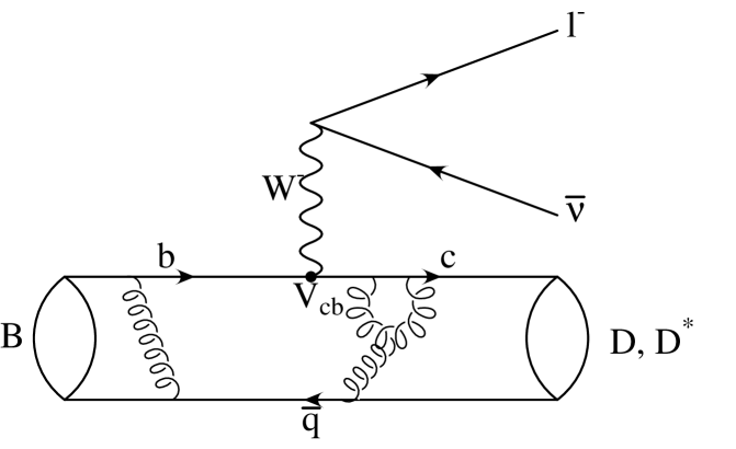
Figure 3: Semi-leptonic decays of a $B$ meson. Here, $l^{-}$ is a lepton and $\bar{\nu}$ is its anti-neutrino.

As was the case for leptonic decays, the fact that the $b$ and the $c$ are confined within hadrons severely modifies their coupling to the $W$.

These semi-leptonic decays are interesting theoretically. They enable one to determine the now famous Isgur-Wise function and to test the range of validity of heavy-quark symmetry. But they are also interesting phenomenologically because they can be used to measure $V_{cb}$. The decay $B\to D^{*}\ell\nu$ is, in fact, very well suited for this task because its rate, aside from being rather large, is free of ${\cal O}\left(\Lambda_{\rm QCD}/m_{c}\right)$-corrections to the heavy-quark symmetry prediction at maximum four-momentum transfer (Luke’s theorem[46]):

$$\frac{1}{\sqrt{\omega^{2}-1}}\frac{d\Gamma(B\to D^{*}\ell\nu)}{d\omega}\buildrel\;\;w\to 1\;\;\over{\longrightarrow}\frac{G_{F}^{2}|V_{cb}|^{2}}{4\pi^{3}}(m_{B}-m_{D^{*}})^{2}m_{D^{*}}^{3}\eta_{A}^{2}\,\left(1+{\cal O}\left(\left(\frac{\Lambda_{\rm QCD}}{m_{c}}\right)^{2}\right)\right)\ ,$$ (34)

where $\omega=v_{B}\cdot v_{D^{*}}$ is the recoil, $v_{B(D^{*})}$ are the four-velocities of the mesons and $\eta_{A}$ are perturbative radiative corrections that will be described shortly. Thus, a measurement of the decay rate very close to the zero-recoil point yields a model-independent determination of $V_{cb}$[4]up to small, non-perturbative ${\cal O}\left(\left(\frac{\Lambda_{\rm QCD}}{m_{c}}\right)^{2}\right)$ corrections. In practice, what one does is to measure the differential decay rate over the whole kinematical range and extrapolate it to $\omega=1$. To be reliable, this extrapolation requires a theoretical guide, especially since the different experiments (ARGUS, CLEO and ALEPH) have been finding decay rates with rather different $\omega$-dependences (see Figs. 13, 14 and 15). This in turn requires a knowledge of the rate’s dependence on $\omega$ which is governed by the non-perturbative QCD dynamics which binds the quarks into mesons. It is here that our lattice calculation enters.

$B\to D\ell\nu$ decays are slightly less well suited for obtaining $V_{cb}$ as they are helicity suppressed, which makes them more difficult to measure close to $\omega=1$. Moreover, their rate is not protected by Luke’s theorem and should suffer larger ${\cal O}\left(\Lambda_{\rm QCD}/m_{c}\right)$ corrections close to zero recoil. Neither of these problems are insurmountable, however, since the rate is far from negligible away from $\omega=1$ and the ${\cal O}\left(\Lambda_{\rm QCD}/m_{c}\right)$ corrections turn out to be parametrically suppressed[4]. So in the future, when better data is available, this channel should also provide a good means for determining $V_{cb}$.

The matrix element required to describe $B\to D\ell\nu$ and $B\to D^{*}\ell\nu$ decays are

$$\frac{\langle D(v^{\prime})|\bar{c}\gamma^{\mu}b|B(v)\rangle}{\sqrt{m_{B}m_{D}}}=(v+v^{\prime})^{\mu}\,h^{+}(\omega)+(v-v^{\prime})^{\mu}\,h^{-}(\omega)\ ,$$ (35)

$$\frac{\langle D^{*}(v^{\prime},\epsilon)|\bar{c}\gamma^{\mu}b|B(v)\rangle}{\sqrt{m_{B}m_{D^{*}}}}=i\epsilon^{\mu\nu\alpha\beta}\epsilon^{*}_{\nu}v^{\prime}_{\alpha}v_{\beta}\,h_{V}(\omega)$$

and

$$\frac{\langle D^{*}(v^{\prime},\epsilon)|\bar{c}\gamma^{\mu}\gamma^{5}b|B(v)\rangle}{\sqrt{m_{B}m_{D^{*}}}}=(\omega+1)\epsilon^{*\mu}\,h_{A_{1}}(\omega)-\epsilon^{*}\cdot v\left(v^{\mu}\,h_{A_{2}}+v^{\prime\mu}\,h_{A_{3}}\right)\ ,$$

where $\omega=v\cdot v^{\prime}$ and $\epsilon^{\mu}$ is the polarization vector of the $D^{*}$.

In the limit that $m_{c}$ and $m_{b}$ are infinite, heavy-quark symmetry reduces the six form factors of Eqs. (35) and (4) to a single universal function of the recoil, $\xi(\omega)$, known as the Isgur-Wise function:

$$h_{+}(\omega)=h_{A_{1}}(\omega)=h_{A_{3}}(\omega)=h_{V}(\omega)=\xi(\omega)$$

and

$$h_{-}(\omega)=h_{A_{2}}(\omega)\equiv 0\ .$$

This symmetry further requires that the Isgur-Wise function be normalized to one at zero recoil[2]:

$$\xi(1)=1\ .$$ (38)

Of course, in nature, the bottom and the charm are not infinitely massive and there are corrections to the simple relations of Eq. (4) as there were to the scaling relation of Eqs. (30) and (32). These corrections can be parametrized in terms of twelve functions $\beta_{i}(\omega)$ and $\gamma_{i}(\omega)$ with $i=+,\ -,\ V,\ A_{1},\ A_{2},\ A_{3}$ such that

$$h_{i}(\omega)=\left(\alpha_{i}+\beta_{i}(\omega)+\gamma_{i}(\omega)\right)\ \xi(\omega)\ ,$$ (39)

where $\alpha_{+}=\alpha_{V}=\alpha_{A_{1}}=\alpha_{A_{3}}=1$ and $\alpha_{-}=\alpha_{2}=0$. The functions $\beta_{i}$ correspond to the exchange of hard gluons across the vector and axial-vector vertices. These corrections are perturbative and in the sequel we use the results obtained by M. Neubert in Ref.[47]. In this reference, Neubert performs a full one-loop matching of HQET to QCD and runs the results at two loops.

The second set of corrections, the $\gamma_{i}$’s, are proportional to inverse powers of the heavy-quark masses $m_{c}$ and $m_{b}$. They correspond to matrix elements of higher-dimension operators in HQET and are therefore non-perturbative and almost as difficult to evaluate as full QCD matrix elements. If most of these corrections cannot be neglected, heavy-quark symmetry obviously loses much of its predictive power. In most cases, heavy-quark symmetry is not a precision tool since leading power corrections are expected to be on the order of $\Lambda_{\rm QCD}/m_{c}\simeq 20\%$. In a few instances, however, heavy-quark symmetry is more constraining as we saw at the beginning of the present section when discussing the extraction of the CKM matrix element $V_{cb}$ and Luke’s theorem.

At the level of form factors, Luke’s theorem guarantees that $h_{+}$ and $h_{A_{1}}$ do not suffer ${\cal O}\left(\Lambda_{\rm QCD}/m_{c,b}\right)$ corrections at zero recoil. Thus

$$\gamma_{+}(1),\ \gamma_{A_{1}}(1)={\cal O}\left(\left(\frac{\Lambda_{\rm QCD}}{m_{c,b}}\right)^{2}\right)$$ (40)

which means that the leading non-perturbative corrections on these form factors ought to be on the order of 4%–i.e., very small.

It is important to emphasize, at this point, that to claim that the Isgur-Wise function, $\xi(\omega)$, has been obtained from any one of the form factors, $h_{i}(\omega)$, one has to convincingly argue that one controls the non-perturbative power corrections, $\gamma_{i}(\omega)$.

4.1 The Form-Factor $h^{+}(\omega)$

The form factor $h^{+}$ dominates the rate for $B\to D\ell\nu$ decays. The matrix element of Eq. (35) which $h^{+}$ parametrizes is obtained from the 3-point function

$$\sum_{{\bf x},{\bf y}}\,e^{-i{\bf q}\cdot{\bf x}}e^{-i{\bf p}^{\prime}\cdot{\bf y}}\,\langle\bar{q}^{R}\gamma_{5}c^{R}_{s}(t_{f},{\bf y})\;\bar{c}^{R}\gamma_{\mu}b^{R}(t,{\bf x})\;\bar{b}^{R}_{s}\gamma_{5}q^{R}(0,{\bf 0})\rangle\ ,$$ (41)

as sketched in Section 2.1. (See Eqs. (25) and (20) for the meaning of subsrcript $s$ and the superscript $R$.)

Since the heavy-quark flavors we consider all have masses in the range of the charm, we do not directly obtain the form factor $h^{+}(\omega)$ relevant for physical $B\to D\ell\nu$ decays. In order to get this physical form factor, we must extrapolate the mass of the initial heavy quark to $m_{b}$ and interporlate the mass of the final heavy quark to $m_{c}$. Thus, we must understand how $h^{+}$ depends on the mass of the initial and final heavy quarks. Since we already understand the dependence on mass which comes from radiative corrections, we study the quantity

$$\frac{h^{+}(\omega)}{1+\beta^{+}(\omega)}\simeq\left(1+\gamma^{+}(\omega)\right)\,\xi(\omega)\ ,$$ (42)

where these corrections are subtracted. In this equation, equality holds only to leading order in power and radiative corrections.

In Fig. 4 we plot the ratio $h^{+}/(1+\beta^{+})$ for four degenerate transitions.

Figure 4: The ratio $h^{+}(\omega)(1+\beta^{+}(\omega))$ is plotted as a function of $\omega$ for four different degenerate transitions corresponding to four values of the heavy-quark mass. The data corresponding to each transition has it’s own symbol as detailed on the plot. The different curves result from individually fitting each set of data to the parametrization $s\xi_{NR}$ (see text). The hopping parameter of the light, spectator antiquark is $\kappa_{q}=0.14144$.

A degenerate transition is one in which the masses of the initial and final heavy quarks are equal. We consider these transitions first, because they are more constrained theoretically[32]. The fact that all four sets of points, which correspond to heavy-quark masses ranging from $1.1{\,\rm GeV}$ to $1.9{\,\rm GeV}$, appear to lie very much on the same curve is a first indication that the heavy-quark-mass dependence of $h^{+}/(1+\beta^{+})$ is very small. That all four sets of data lie on the same curve can actually be shown by fitting each set individually to a standard parametrization for the Isgur-Wise function and showing that the parameters of the resulting curves are equal within statistical errors. The parametrization we use is[48]

$$\xi_{NR}(\omega)=\frac{2}{\omega+1}\;{\rm exp}\left[-(2\rho^{2}-1)\,\frac{\omega-1}{\omega+1}\right]\ ,$$ (43)

where $\rho^{2}$ is the negative of the slope of the function $\xi_{NR}$ at $\omega=1$ and is the parameter of this fitting function. We acutally fit the data to $s\,\xi_{NR}$ where $s$ is a parameter which allows us to test how well we have normalized our data. If our data is well normalized and $\xi_{NR}$ is a valid parametrization for the data, then $s$ ought to be equal to 1. For all four sets of data, we find $s=0.99(1)$ and $\rho^{2}=1.4$ where the error on $s$ is statistical and the statistical errors on $\rho^{2}$ are the order of $0.2$ but differ slighly from data set to data set. Thus, our data appears to be correctly normalized and independent of heavy-quark mass.

This mass dependence can in fact be quantified by extracting the power corrections, $\gamma^{+}$, from our data. If radiative corrections are neglected, these power corrections can be parametrized in terms of a single universal function, $g(\omega)$, such that

$$\gamma^{+}(\omega)=g(\omega)\,\frac{\bar{\Lambda}}{2}\,\left(\frac{1}{m_{b}}+\frac{1}{m_{c}}\right)+{\cal O}\left(\left(\frac{\bar{\Lambda}}{2m_{c,b}}\right)^{2}\right)\ ,$$ (44)

where $\bar{\Lambda}$ is the energy carried by the light degrees of freedom and is approximately equal to $500{\,\rm MeV}$ when the light quark $q$ is an up or down quark[4]. Furthermore, according to Luke’s theorem,

$$g(1)=0\ .$$ (45)

The form factor, $g(\omega)$, can be extracted from our results for $h^{+}$ by taking ratios of the quantity $h^{+}/(1+\beta^{+})$ at fixed $\omega$ but different values of the initial or final heavy quark mass (see Eq. (42)). Because lattice momenta are quantized, there are, in our data, only four values of $\omega$ for which this can be done. These four point are plotted in Fig. 5.

Figure 5: The subleading form factor, $g(\omega)$, is plotted versus $\omega$. The hopping parameter of the light, spectator antiquark is $\kappa_{q}=0.14144$.

This figure indicates that $g(\omega)$ is consistent with 0 and in any case is less than one or two times $10^{-1}$ in the range of recoils that we can explore. Since $(\bar{\Lambda}/2)(1/m_{b}+1/m_{c})$ is about 0.4 for the quarks we simulate power corrections to $h^{+}$ appear to be indeed very small. When combined with the information obtained earlier for degenerate transitions which covered a much larger range of recoils, this result clearly confirms that $h^{+}/(1+\beta^{+})$ depends very little on heavy-quark mass. This weak dependence on heavy-quark mass, however, can be interpreted in many ways. A first explanation is that power corrections to $h^{+}$, as well as discretization errors proportional to the masses of the heavy quarks, are genuinely small. A second possible interpretation is that discretization errors are small but that the ${\cal O}\left(\bar{\Lambda}/2m_{b,c}\right)$-correction happens to cancel against the higher order power corrections in the range of heavy-quark mass that we are investigating–i.e. that in this range of masses the heavy quark regime has not yet been reached. A third is that the power corrections and discretization errors have opposite signs and cancel. Since the cancellations of options two and three would have to take place over a rather large range of recoils and a rather large range of heavy-quark masses, they seem quite unlikely. So in what follows, we will adopt the interpretation that power corrections to $h^{+}$ are genuinely small even for heavy quark with mass close to that of the charm.

The absence of heavy-quark mass dependence of the ratio $h^{+}/(1+\beta^{+})$ also means that to a good approximation we have obtained the infinite mass result. Thus, we can combine all of our data for $h^{+}/(1+\beta^{+})$ for fixed light-quark mass but all possible initial and final heavy-quark masses and call the resulting function an Isgur-Wise function (see Eq. (42)). In Fig. 6, we plot this combined data for the case where the mass of the light antiquark is interpolated to the strange-quark mass.

Figure 6: The ratio $h^{+}/(1+\beta^{+})$ is plotted as a function of $\omega$. The different symbols correspond to different initial and/or final heavy-quark masses. All symbols, however, correspond to situations where the light antiquark has the mass of the strange. Because this ratio exhibits no dependence on heavy-quark mass, it is just the Isgur-Wise function $\xi_{s}(\omega)$. The solid curve depicts the result of fitting the parametrization $s\xi_{NR}$ to the data.

The resulting Isgur-Wise function, which we denote by $\xi_{s}(\omega)$, is relevant to the decays $B_{s}\to D_{s}\ell\nu$ and $B_{s}\to D_{s}^{*}\ell\nu$ and elastic $B_{s}$ and $D_{s}$ scattering off a photon. The different symbols on the plot correspond to different initial and/or final heavy-quark mass. The fact that these different symbols often lie on top of each other and always appear to lie on the same curve is again confirmation that the mass dependence of the ratio $h^{+}/(1+\beta^{+})$ is very small. The solid line in Fig. 6 corresponds to a fit of the data to the parametrization $s\xi_{NR}(\omega)$, with $\xi_{NR}$ given in Eq. (43). From this fit we find that this Isgur-Wise function has a slope of $-\rho^{2}_{s}$ at $\omega=1$ with

$$\rho^{2}_{s}=1.2\raisebox{0.80002pt}{\scriptsize{$\;\begin{array}[]{@{}l@{}}\makebox[15.0pt][c]{$+$}\makebox[3.85002pt][r]{2}\\[-0.83997pt] \makebox[15.0pt][c]{$-$}\makebox[3.85002pt][r]{2}\end{array}$}}({\rm stat.})\raisebox{0.80002pt}{\scriptsize{$\;\begin{array}[]{@{}l@{}}\makebox[15.0pt][c]{$+$}\makebox[3.85002pt][r]{2}\\[-0.83997pt] \makebox[15.0pt][c]{$-$}\makebox[3.85002pt][r]{1}\end{array}$}}({\rm syst.})$$ (46)

where the sytematic error was obtained in a way described in Ref.[32].

In Fig. 7 we repeat the same exercise with the light-quark mass extrapolated to the chiral limit.

Figure 7: The ratio $h^{+}/(1+\beta^{+})$ is plotted as a function of $\omega$. The different symbols correspond to different initial and/or final heavy-quark masses. All symbols, however, correspond to situations where the light antiquark is massless. Because this ratio exhibits no dependence on heavy-quark mass, it is just the Isgur-Wise function $\xi_{u,d}(\omega)$. The solid curve depicts the result of fitting the parametrization $s\xi_{NR}$ to the data.

The Isgur-Wise function obtained thus is the one relevant to the decays $B\to D\ell\nu$ and $B\to D^{*}\ell\nu$ and elastic $B$ and $D$ scattering. This function is traditionally called “the Isgur-Wise function”. Performing the same fit as in Fig. 6, we find that the corresponding slope parameter is

$$\rho^{2}_{u,d}=0.9\raisebox{0.80002pt}{\scriptsize{$\;\begin{array}[]{@{}l@{}}\makebox[15.0pt][c]{$+$}\makebox[3.85002pt][r]{2}\\[-0.83997pt] \makebox[15.0pt][c]{$-$}\makebox[3.85002pt][r]{3}\end{array}$}}({\rm stat.})\raisebox{0.80002pt}{\scriptsize{$\;\begin{array}[]{@{}l@{}}\makebox[15.0pt][c]{$+$}\makebox[3.85002pt][r]{4}\\[-0.83997pt] \makebox[15.0pt][c]{$-$}\makebox[3.85002pt][r]{2}\end{array}$}}({\rm syst.})\ .$$ (47)

This slope parameter, as well as the one of Eq. (46) is compared with the predictions of other authors in Table 5. Our predictions lie safely above the lower bound of Bjorken[49] and below the upper bound of de Rafael and Taron[50]. Our results for $\rho^{2}_{s}$ also agree with the lattice result of[51] although the details and systematics of the two calculations are different. The authors of [51] do not quote a value of $\rho^{2}_{u,d}$ for vanishing light-quark mass because of their poor statistics in the chiral limit.

Reference	$-\xi^{\prime}_{u,d}(1)$	$-\xi^{\prime}_{s}(1)$
UKQCD	$0.9\raisebox{0.80002pt}{\scriptsize{$\;\begin{array}[]{@{}l@{}}\makebox[15.0pt][c]{$+$}\makebox[3.85002pt][r]{2}\\[-0.83997pt] \makebox[15.0pt][c]{$-$}\makebox[3.85002pt][r]{3}\end{array}$}}({\rm stat.})\raisebox{0.80002pt}{\scriptsize{$\;\begin{array}[]{@{}l@{}}\makebox[15.0pt][c]{$+$}\makebox[3.85002pt][r]{4}\\[-0.83997pt] \makebox[15.0pt][c]{$-$}\makebox[3.85002pt][r]{2}\end{array}$}}({\rm syst.})$	$1.2\raisebox{0.80002pt}{\scriptsize{$\;\begin{array}[]{@{}l@{}}\makebox[15.0pt][c]{$+$}\makebox[3.85002pt][r]{2}\\[-0.83997pt] \makebox[15.0pt][c]{$-$}\makebox[3.85002pt][r]{2}\end{array}$}}({\rm stat.})\raisebox{0.80002pt}{\scriptsize{$\;\begin{array}[]{@{}l@{}}\makebox[15.0pt][c]{$+$}\makebox[3.85002pt][r]{2}\\[-0.83997pt] \makebox[15.0pt][c]{$-$}\makebox[3.85002pt][r]{1}\end{array}$}}({\rm syst.})$
Bernard, Shen and Soni[51]		1.24(26)(stat.)(26)(syst.)
de Rafael and Taron[50]	$\rho^{2}<1.42$
Close and Wambach[53]	1.40	1.64
Neubert[4]	0.66(5)
Voloshin[55]	1.4(3)
Bjorken[49]	$\rho^{2}>0.25$
Blok and Shifman[56]	$0.35<\rho^{2}<1.15$
Høgaasen and Sadzikowski[57]	0.98	1.135
Rosner[58]	1.59(43)
Burdman[59]	1.08(10)
Dai, Huang and Jin[60]	1.05(20)
Experiment (see text)	0.87(12)(20)

Table 5: Comparison of our lattice results for $-\xi^{\prime}_{u,d}(1)$ and $-\xi^{\prime}_{s}(1)$ to the theoretical predictions of various authors and to experiment.

Also for comparison, we quote an average experimental value for the slope of the Isgur-Wise function compiled by Neubert[52] from very recent results of the ALEPH[61] and CLEO[62] Collaborations as well as older data from the ARGUS Collaboration[63]:

$$\rho^{2}_{u,d(expt.)}=0.87(12)(20)\ ,$$ (48)

where the second error is theoretical and accounts for the uncertainty in the size of $1/m_{c}$ corrections[52]. Agreement with our result is excellent (see Eq. (47)). Such good agreement, however, is most certainly coincidental given the size of both the experimental and lattice errors.

As can be inferred from our determinations of $\rho^{2}_{u,d}$ and $\rho^{2}_{s}$ (Eqs. (47) and (46)) our results suggest that $\rho^{2}$ decreases slightly as light-quark mass decreases. Such a decrease is consistent with one’s intuition about the inertia of the light degrees of freedom. A very similar trend is also found by H. Høgaasen and M. Sadzikowski[57]. In fact, our predictions for $\rho^{2}$ itself are in excellent agreement with theirs. Their prediction is based on an improved bag model calculation and is an extension of earlier work by M. Sadzikowski and K. Zalewski[64]. A similar decrease in slope with spectator-quark mass is observed by F. E. Close and A. Wambach[53] though the values they quote for $\rho^{2}_{u,d}$ and $\rho^{2}_{s}$ are slightly larger than the ones we find.

I wish to mention, finally, that J. Mandula and M. Ogilvie are in the process of calculating the Isgur-Wise function using the lattice version of HQET whose action was given in Eq. (22)[54].

4.2 The Form Factor $h_{A_{1}}(\omega)$

We now turn to the subject of $B\to D^{*}\ell\nu$ decays. Here the dominant form factor is $h_{A_{1}}$. This form factor is obtained from the 3-point function

$$\sum_{{\bf x},{\bf y}}\,e^{-i{\bf q}\cdot{\bf x}}e^{-i{\bf p}^{\prime}\cdot{\bf y}}\,\langle\bar{q}^{R}\gamma_{5}c^{R}_{s}(t_{f},{\bf y})\;\bar{c}^{R}\gamma_{\mu}\gamma_{5}b^{R}(t,{\bf x})\;\bar{b}^{R}_{s}\gamma_{5}q^{R}(0,{\bf 0})\rangle\ ,$$ (49)

as $h^{+}$ was from the 3-point function of Eq. (41). Here again, we must study the behavior of the form factor with heavy-quark mass to obtain the form factor relevant for physical $B\to D^{*}\ell\nu$ decays since our simulation is performed with heavy-quark masses in the range of the charm-quark mass. We do so by considering the quantity

$$\frac{h_{A_{1}}(\omega)}{1+\beta_{A_{1}}(\omega)}\simeq\left(1+\gamma_{A_{1}}(\omega)\right)\,\xi(\omega)\ ,$$ (50)

where the equality holds only to leading order in power and radiative corrections.

The analysis we perform of the quantity $h_{A_{1}}/(1+\beta_{A_{1}})$ parallels the analysis of $h^{+}/(1+\beta^{+})$ carried out in Section 4.1. In Fig. 8 we plot the ratio $h_{A_{1}}/(1+\beta_{A_{1}})$ for four degenerate transitions.

Figure 8: The ratio $h_{A_{1}}/(1+\beta_{A_{1}})$ is plotted as a function of $\omega$ for four different degenerate transitions corresponding to four values of the heavy-quark mass. The data corresponding to each transition has it’s own symbol as detailed on the plot. The different curves result from individually fitting each set of data to the parametrization $s\xi_{NR}$ (see text). The hopping parameter of the light, spectator antiquark is $\kappa_{q}=0.14144$.

Here too we fit the data for each individual degenerate transition to the parametrization $s\,\xi_{NR}(\omega)$, with $\xi_{NR}(\omega)$ given in Eq. (43). We find $s=1.00(2)$ and $\rho^{2}=1.3$ with a statistical error on the order of $0.3$ for all four data sets. This confirms the naked eye impression that all four data sets lie on the same curve and thus indicates that the dependence of the ratio $h_{A_{1}}/(1+\beta_{A_{1}})$ on heavy-quark mass is very small in the range of masses we are considering. Moreover, the fact that the curves on which all of these points lie are almost the same as those found for $h^{+}/(1+\beta^{+})$ is a first indication that the spin component of the heavy-quark symmetry is unbroken in this case even in the region of the charm-quark mass.

As we did for $h^{+}/(1+\beta^{+})$, we can try to quantify the heavy-quark mass dependence of the ratio $h_{A_{1}}/(1+\beta_{A_{1}})$ by measuring the power corrections to this ratio. If radiative corrections are neglected, the power corrections to $h_{A_{1}}$ can be parametrized in terms of the three univsersal functions $g(\omega)$, $\eta(\omega)$ and $g^{*}(\omega)$:

$$\gamma_{A_{1}}=\frac{\bar{\Lambda}}{2m_{b}}\,\left(g(\omega)+\frac{\omega-1}{\omega+1}\left(1-2\,\eta(\omega)\right)\right)+\frac{\bar{\Lambda}}{2m_{c}}\,\left(g^{*}(\omega)+\frac{\omega-1}{\omega+1}\right)+{\cal O}\left(\left(\frac{\bar{\Lambda}}{2m_{c,b}}\right)^{2}\right)\ ,$$ (51)

where $g(\omega)$ is the same form factor that appears in the power corrections to $h^{+}$ in Eq. (44). Here again, Luke’s theorem requires that the ${\cal O}\left(\bar{\Lambda}/2m_{b,c}\right)$ power corrections to $h_{A_{1}}$ to vanish at $\omega=1$. This means that $g^{*}(\omega)$ must vanish at $\omega=1$:

$$g^{*}(1)=0\ .$$ (52)

$\eta$, however, is unconstrained because it does not appear in the expression for power corrections at $\omega=1$.

We extract the functions which multiply the expansion parameters $\bar{\Lambda}/(2m_{b,c})$ in Eq. (51) by taking ratios of the quantity $h_{A_{1}}/(1+\beta_{A_{1}})$ at fixed $\omega$ and light-quark mass but different values of the initial or final heavy-quark mass. We plot our results in Fig. 9.

Figure 9: Power corrections to the form factor $h_{A_{1}}$. Plotted are the functions which multiply the expansion parameters $\bar{\Lambda}/(2m_{b,c})$ in Eq. (51). The hopping parameter of the light, spectator antiquark is $\kappa_{q}=0.14144$.

Both these functions are consistent with 0 and are less than one or two times $10^{-1}$ in the range of recoils that we can explore. Since these functions are themselves multiplied by the small expansion parameters $\bar{\Lambda}/(2m_{c})$ and $\bar{\Lambda}/(2m_{b})$ which are on the order of 0.2 for the quarks we simulate, the power corrections to $h_{A_{1}}$ are very small (on the order of 4% or less) in the explored range of recoils. Together with the information provided by the fits in Fig. 8, this results indicates that power corrections to $h_{A_{1}}$ are very small for all $\omega$, up to the caveats mentioned in Section 4.1 in the discussion on power corrections to $h^{+}$.

The fact that $h_{A_{1}}/(1+\beta_{A_{1}})$ depends very little on heavy-quark mass means, as it did for the ratio $h^{+}/(1+\beta^{+})$, that our results are to a very good approximation infinite mass results. So again we can combine all of our data for a given light-quark mass to obtain the Isgur-Wise functions $\xi_{s}$ and $\xi_{u,d}$ which are in principle the same functions as the ones given by the ratio $h^{+}/(1+\beta^{+})$. We plot these form factors as functions of the four-velocity recoil in Figs. 10 and 11.

Figure 10: The ratio $h_{A_{1}}/(1+\beta_{A_{1}})$ is plotted as a function of $\omega$. The different symbols correspond to different initial and/or final heavy-quark masses. All symbols, however, correspond to situations where the light antiquark has the mass of the strange. Because this ratio exhibits no dependence on heavy-quark mass, it is just the Isgur-Wise function $\xi_{s}(\omega)$. The solid curve depicts the result of fitting the parametrization $s\xi_{NR}$ to the data.

Figure 11: The ratio $h_{A_{1}}/(1+\beta_{A_{1}})$ is plotted as a function of $\omega$. The different symbols correspond to different initial and/or final heavy-quark masses. All symbols, however, correspond to situations where the light antiquark is massless. Because this ratio exhibits no dependence on heavy-quark mass, it is just the Isgur-Wise function $\xi_{u,d}(\omega)$. The solid curve depicts the result of fitting the parametrization $s\xi_{NR}$ to the data.

The solid curve in both these plots result from fitting our data to the parametrization $s\xi_{NR}$. These fits, give the following slope parameters:

$$\rho^{2}_{s}=1.2\raisebox{0.80002pt}{\scriptsize{$\;\begin{array}[]{@{}l@{}}\makebox[15.0pt][c]{$+$}\makebox[3.85002pt][r]{3}\\[-0.83997pt] \makebox[15.0pt][c]{$-$}\makebox[3.85002pt][r]{3}\end{array}$}}({\rm stat.})\raisebox{0.80002pt}{\scriptsize{$\;\begin{array}[]{@{}l@{}}\makebox[15.0pt][c]{$+$}\makebox[3.85002pt][r]{7}\\[-0.83997pt] \makebox[15.0pt][c]{$-$}\makebox[3.85002pt][r]{1}\end{array}$}}({\rm syst.})$$ (53)

and

$$\rho^{2}_{u,d}=0.9\raisebox{0.80002pt}{\scriptsize{$\;\begin{array}[]{@{}l@{}}\makebox[15.0pt][c]{$+$}\makebox[3.85002pt][r]{4}\\[-0.83997pt] \makebox[15.0pt][c]{$-$}\makebox[3.85002pt][r]{5}\end{array}$}}({\rm stat.})\raisebox{0.80002pt}{\scriptsize{$\;\begin{array}[]{@{}l@{}}\makebox[15.0pt][c]{$+$}\makebox[3.85002pt][r]{9}\\[-0.83997pt] \makebox[15.0pt][c]{$-$}\makebox[3.85002pt][r]{1}\end{array}$}}({\rm syst.})\ .$$ (54)

These slopes are precisely the ones we found for the ratio $h^{+}/(1+\beta^{+})$ (see Eqs. (46) and (47)). The Isgur-Wise functions obtained from $h_{A_{1}}$ and $h^{+}$ are in fact equal over the whole range of recoils to within less than 4%, as can be seen in Fig. 12 where we plot the ratio $h_{A_{1}}(1+\beta^{+})/h^{+}(1+\beta_{A_{1}})$.

Figure 12: The ratio of the Isgur-Wise functions obtained from $h^{+}$ and $h_{A_{1}}$ is plotted as a function of $\omega$. Only degenerate transitions are considered. The different symbols correspond to different values of the heavy quark’s mass. All symbols, however, correspond to situations where the light antiquark has a hopping parameter $\kappa_{q}=0.14144$. The points are very close to one, as they should be if heavy-quark symmetry is respected.

What has emerged is a very consistent picture of $B\to D\ell\nu$ and $B\to D^{*}\ell\nu$ decays in which heavy-quark symmetry is surprisingly well satisfied even though the heavy quarks with which we work have masses in the range of the charm-quark mass. This is in stark contrast with the results for the decay constant $f_{P}$ presented in Section 3.1 where we found that corrections to the heavy-quark limit were on the order of 30% for these same heavy quarks. What seems to be happening here is that the protection from ${\cal O}\left(\bar{\Lambda}/2m_{b,c}\right)$-corrections that Luke’s theorem provides at zero recoil appears to extend over the full range of recoils so that corrections which one would naively expect to be on the order of $(\bar{\Lambda}/2)(1/m_{c}+1/m_{b})\simeq 30-40\%$ for the quarks we are studying turn out to be on the order of a few percent.

4.3 Extraction of $V_{cb}$

When power corrections and radiative corrections for $\omega>1$ are neglected, the differential decay rate for $B\to D^{*}\ell\nu$ decays is given by

$$\frac{1}{\sqrt{\omega^{2}-1}}\frac{d\Gamma(B\to D^{*}\ell\nu)}{d\omega}\simeq\frac{G_{F}^{2}|V_{cb}|^{2}}{4\pi^{3}}(m_{B}-m_{D^{*}})^{2}m_{D^{*}}^{3}\eta_{A}^{2}\,(1+\delta_{1/m^{2}})\,\xi_{u,d}(\omega)\ ,$$ (55)

where $\delta_{1/m^{2}}$ stands for the power corrections to $h_{A_{1}}$ at $\omega=1$ which have been the object of much controversy lately[52, 65]. Having determined $\xi_{u,d}$ with our lattice calculation, the only unknown left in Eq. (55) is the CKM matrix element $|V_{cb}|$. Thus, a fit of the theoretical expression of Eq. (55) to an experimental measurement of the rate immdediately yields a measurement of $|V_{cb}|$. This is what we do in Fig. 13 where we use very recent data obtained by the CLEO collaboration[62].

Figure 13: $\chi^{2}$-fit of the expression $|V_{cb}|\,\eta_{A}\,\xi_{u,d}(\omega)(1+\delta_{1/m^{2}})$ to the experimental data for this quantity obtained by the CLEO Collaboration [62]. In this fit, the function $\xi_{u,d}(\omega)$ is fixed to our lattice prediction, i.e. to $\xi_{NR}$ with $\rho^{2}$ given by Eq. (47). The fit parameter is $|V_{cb}|\,\eta_{A}\,(1+\delta_{1/m^{2}})$. The UKQCD data and curve are just those of Fig. 7 appropriately rescaled by the fit parameter. The experimental data assumes $\tau_{B^{0}}=1.53(9)\mbox{ps}$ and $\tau_{B^{+}}=1.68(12)\mbox{ps}$.

The value of $|V_{cb}|$ that this fit gives is

$$|V_{cb}|=0.037\raisebox{0.80002pt}{\scriptsize{$\;\begin{array}[]{@{}l@{}}\makebox[15.0pt][c]{$+$}\makebox[3.85002pt][r]{1}\\[-0.83997pt] \makebox[15.0pt][c]{$-$}\makebox[3.85002pt][r]{1}\end{array}$}}\raisebox{0.80002pt}{\scriptsize{$\;\begin{array}[]{@{}l@{}}\makebox[15.0pt][c]{$+$}\makebox[3.85002pt][r]{2}\\[-0.83997pt] \makebox[15.0pt][c]{$-$}\makebox[3.85002pt][r]{2}\end{array}$}}\raisebox{0.80002pt}{\scriptsize{$\;\begin{array}[]{@{}l@{}}\makebox[15.0pt][c]{$+$}\makebox[3.85002pt][r]{4}\\[-0.83997pt] \makebox[15.0pt][c]{$-$}\makebox[3.85002pt][r]{1}\end{array}$}}\;\left(\frac{0.99}{\eta_{A}}\right)\frac{1}{1+\delta_{1/m^{2}}}\ ,$$ (56)

where the first set of errors is due to the experimental uncertainties, the second set of errors to the statistical errors in our determination of the Isgur-Wise function and the third to our systematic errors. A similar fit to ALEPH data[61] gives (see Fig. 14)

Figure 14: Same fit as in Fig. 13 but to data of ALEPH[61] which assumes $\tau_{B^{0}}=1.53(9)\mbox{ps}$.

$$|V_{cb}|=0.042\raisebox{0.80002pt}{\scriptsize{$\;\begin{array}[]{@{}l@{}}\makebox[15.0pt][c]{$+$}\makebox[3.85002pt][r]{2}\\[-0.83997pt] \makebox[15.0pt][c]{$-$}\makebox[3.85002pt][r]{2}\end{array}$}}\raisebox{0.80002pt}{\scriptsize{$\;\begin{array}[]{@{}l@{}}\makebox[15.0pt][c]{$+$}\makebox[3.85002pt][r]{2}\\[-0.83997pt] \makebox[15.0pt][c]{$-$}\makebox[3.85002pt][r]{3}\end{array}$}}\raisebox{0.80002pt}{\scriptsize{$\;\begin{array}[]{@{}l@{}}\makebox[15.0pt][c]{$+$}\makebox[3.85002pt][r]{4}\\[-0.83997pt] \makebox[15.0pt][c]{$-$}\makebox[3.85002pt][r]{1}\end{array}$}}\;\sqrt{\frac{1.53{\rm ps}}{\tau_{B}}}\left(\frac{0.99}{\eta_{A}}\right)\frac{1}{1+\delta_{1/m^{2}}}\ ,$$ (57)

and to ARGUS data[63] (see Fig. 15),

Figure 15: Same fit as in Fig. 13 but to data of the ARGUS Collaboration[63] which assumes $\tau_{B^{0}}=1.53(9)\mbox{ps}$.

$$|V_{cb}|=0.033\raisebox{0.80002pt}{\scriptsize{$\;\begin{array}[]{@{}l@{}}\makebox[15.0pt][c]{$+$}\makebox[3.85002pt][r]{2}\\[-0.83997pt] \makebox[15.0pt][c]{$-$}\makebox[3.85002pt][r]{2}\end{array}$}}\raisebox{0.80002pt}{\scriptsize{$\;\begin{array}[]{@{}l@{}}\makebox[15.0pt][c]{$+$}\makebox[3.85002pt][r]{1}\\[-0.83997pt] \makebox[15.0pt][c]{$-$}\makebox[3.85002pt][r]{2}\end{array}$}}\raisebox{0.80002pt}{\scriptsize{$\;\begin{array}[]{@{}l@{}}\makebox[15.0pt][c]{$+$}\makebox[3.85002pt][r]{3}\\[-0.83997pt] \makebox[15.0pt][c]{$-$}\makebox[3.85002pt][r]{1}\end{array}$}}\;\sqrt{\frac{1.53{\rm ps}}{\tau_{B}}}\left(\frac{0.99}{\eta_{A}}\right)\frac{1}{1+\delta_{1/m^{2}}}\ .$$ (58)

These results for $|V_{cb}|$ must not be taken too literally because the experimental measurements are binned according to slightly biased estimators of the recoil and because we have neglected small $1/m_{b,c}$ and radiative corrections for $\omega>1$. Neverthless, it is clear from Fig. 13, Fig. 14 and Fig. 15 that our prediction is consistent with experiment and favors slightly the data of CLEO and ALEPH over that of ARGUS.

4.4 The Form Factor $h_{V}(\omega)$

We now briefly turn to the form factor $h_{V}$ defined in Eq. (4). This form factor is interesting because it is not protected by Luke’s theorem as are $h^{+}$ and $h_{A_{1}}$. This means that one would expect power corrections to this form factor to be more in line with naive expectations.

We have very prelimary results for the form factor $h_{V}$ and it does indeed seem to exhibit power corrections on the order of 20 to 40% depending on the heavy-quarks considered. It is unclear, however, what fraction of these corrections are true $1/m_{b,c}$-corrections and what fraction are $am_{Q}$ discretization errors. The problem here is that we cannot subtract these discretization errors as we did for $h^{+}$ and $h_{A_{1}}$ (see Ref. [32] for details), because there is no normalization condition for $h_{V}$.

So instead of presenting results which may suffer from large discretization errors, we will present a framework in which the form factor $h_{V}$ may be analyzed once these errors are controlled. As we did for these two other form factors, we should study $h_{V}$ with the radiative corrections taken out:

$$\frac{h_{V}(\omega)}{1+\beta_{V}(\omega)}\simeq(1+\gamma_{V}(\omega))\,\xi(\omega)\ ,$$ (59)

where $\gamma_{V}$ labels power corrections. These corrections can be parametrized by the three universal functions $g$, $g^{*}$ and $\eta$ that we encountered in Section 4.1 and Section 4.2. In the absence of radiative corrections,

$$\gamma_{V}=\frac{\bar{\Lambda}}{2m_{b}}\,\left(g(\omega)+(1-2\,\eta(\omega))\right)+\frac{\bar{\Lambda}}{2m_{c}}\,\left(g^{*}(\omega)+1\right)+{\cal O}\left(\left(\frac{\bar{\Lambda}}{2m_{c,b}}\right)^{2}\right)\ .$$ (60)

Then, by considering ratios of the quantity $h_{V}/(1+\beta_{V})$ for fixed $\omega$ and light-quark mass, but different heavy-quark masses, we would extract the functions $g(\omega)+(1-2\,\eta(\omega))$ and $g^{*}(\omega)+1$. We would expect both these functions to be of ${\cal O}\left(1\right)$ since there is no symmetry, here, which forbids the appearance of power corrections. It is interesting to note that this expectation is consistent with the statement that $g^{*}(\omega)$ must vanish at $\omega=1$ (see Eq. (52)).

Having obtained these functions, we would combine them with the results for the power corrections to $h^{+}$ and $h_{A_{1}}$ of Figs. 5 and 9 and solve the resulting system of equations at fixed $\omega$ for the subleading universal functions $g$, $g^{*}$ and $\eta$.

We have actually carried out this whole procedure on our preliminary data and find results for $g$, $g^{*}$ and $\eta$ which are very much in line with what one can infer from sumrule calculations[4].

5 Penguins on the Lattice

We now turn to the study of $B\to K^{*}\gamma$ decays. These decays occur through the quark level process $b\to s\gamma$ depicted in Fig. 16 which mediated by a flavor-changing-neutral-current (FCNC).

Figure 16: Example of a penguin diagram that contributes to the decay $b\to s\gamma$.

Such FCNC processes are interesting because they are fobidden at tree level in the Standard Model and only occur at one or higher-loop order. Their study therefore provides a means for testing the details of the Standard Model. And because even at lowest order they are sensitive to the presence of new particles that may appear in the loops of their diagrams, they may even give us a handle on physics beyond the Standard Model at comparatively low energies. In fact, bounds on the $b\to s\gamma$ branching ratio have already been used to place constraints on supersymmetric as well as non-supersymmetric extensions to the Standard Model. A comprehensive review of these results can be found in Ref.[67].

Another interesting aspect of $b\to s\gamma$ decays is that they may permit a measurement of the poorly determined CKM matrix element $V_{ts}$.

Experimentally, $b\to s\gamma$ decays are difficult for the same reasons that make them interesting theoretically. They occur at one loop and their rate is suppressed by two powers of the Fermi constant $G_{F}$: they are rare decays. Nevertheless, the CLEO Collaboration has been able to measure the branching ratio for the exclusive channel $B\to K^{*}\gamma$. It found that this decay has a branching ratio[7]

$${\cal BR}\left(B\to K^{*}\gamma\right)=(4.5\pm 1.5\pm 0.9)\times 10^{-5}\ .$$ (61)

In order to compare this very pretty experimental result with the predictions of the Standard Model, one has to compute the long-distance contributions of the strong interaction which are, of course, non-perturbative. These long-distance contributions are given by the hadronic matrix element $\langle K^{*}|\,\bar{s}\sigma_{\mu\nu}q^{\mu}(1+\gamma_{5})b\,|B\rangle$ which can be parametrized by three form factors[68]

$$\langle K^{*}(k,\epsilon)|\,\bar{s}\sigma_{\mu\nu}q^{\nu}\frac{(1+\gamma_{5})}{2}b\,|B(p)\rangle=\sum_{i=1}^{3}C^{i}_{\mu}T_{i}(q^{2}),$$ (62)

where $k$ and $\epsilon$ are the momentum and polarization vectors of the $K^{*}$; $p$ is the momentum of the $B$; $q=p-k$; and

$$C^{1}_{\mu} = 2\varepsilon_{\mu\nu\lambda\rho}\epsilon^{\nu}p^{\lambda}k^{\rho},$$ (63)

$$C^{2}_{\mu} = i\epsilon_{\mu}(m_{B}^{2}-m_{K^{*}}^{2})-i\epsilon\cdot q(p+k)_{\mu},$$ (64)

$$C^{3}_{\mu} = i\epsilon\cdot q\left(q_{\mu}-\frac{q^{2}}{m_{B}^{2}-m_{K^{*}}^{2}}(p+k)_{\mu}\right).$$ (65)

On the lattice, these form factors are obtained from a 3-point function in very much the same way as were the semi-leptonic form factors of Section 4. The viability of this particular calculation was first demonstrated by Bernard, Hsieh and Soni in Ref.[68].

As the photon emitted is on-shell, the form factors need only be evaluated at $q^{2}{=}0$. In this limit,

$$T_{2}(q^{2}{=}0)=T_{1}(q^{2}{=}0),$$ (66)

and the coefficient of $T_{3}(q^{2}{=}0)$ vanishes. Hence, the branching ratio can be expressed in terms of a single number which we take to be $T_{1}(q^{2}{=}0)$.

As in our studies of leptonic and semi-leptonic decays of $B$ mesons, the simulation is performed with the four heavy quarks listed in Table 3. Since these quarks have masses around that of the charm, results have to be extrapolated to $m_{b}$. Here, however, the dependence of the relevant form factors on heavy-quark mass is not as straighforward as it was for leptonic decay constants and semi-leptonic form factors because the light degrees of freedom in this decay have momenta comparable to the mass of the $b$-quark in large sections of phase space. Nevertheless, in a region around $q^{2}_{max}=(m_{B}-m_{K^{*}})^{2}$ heavy-quark symmetry will apply. In that region, one finds that $T_{1}(q^{2})$ and $T_{2}(q^{2})$ scale according to[70]:

$$T_{1}\left(q^{2}\simeq q^{2}_{max};m_{P};m_{K^{*}}\right)=a_{0}\sqrt{m_{P}}\times[\alpha_{s}(m_{P})]^{-2/\beta_{0}}\left(1+\frac{a_{1}}{m_{P}}+\frac{a_{2}}{m_{P}^{2}}+\dots\right)$$ (67)

and

$$T_{2}\left(q^{2}\simeq q^{2}_{max};m_{P};m_{K^{*}}\right)=b_{0}\frac{1}{\sqrt{m_{P}}}\times[\alpha_{s}(m_{P})]^{-2/\beta_{0}}\left(1+\frac{b_{1}}{m_{P}}+\frac{b_{2}}{m_{P}^{2}}+\dots\right)\ ,$$ (68)

with the same one-loop running coupling $\alpha_{s}$ and the same $\beta_{0}$ as for the leptonic case (see comments after Eq. (30)).

The problem now is to find a way to use these scaling relations to get $T_{1}\left(q^{2}{=}0;m_{B};m_{K^{*}}\right)$. The first approach is to:

1. extrapolate the direct measurements of $T_{2}\left(q^{2}=q^{2}_{max};m_{P};m_{K^{*}}\right)$ to $m_{P}=m_{B}$;

2. use the results for this form factor at fixed $m_{P}\simeq m_{D}$ to make an educated guess about its behavior in $q^{2}$ at $m_{B}$;

3. use this behavior to extrapolate the value of $T_{2}\left(q^{2}=q^{2}_{max};m_{B};m_{K^{*}}\right)$ obtained in step 1 to $q^{2}=0$.

This method has the advantage that it only requires knowledge of $T_{2}$’s $q^{2}$ dependence at $m_{B}$. Its disadvantage, however, is that one has to extrapolate $T_{2}$ over a wide range of momentum transfers from $q^{2}=q^{2}_{max}$ to $q^{2}=0$. Since one does not exactly know the functional behavior of $T_{2}$ in $q^{2}$, this extrapolation leads to rather large uncertainties. Bernard, Hsieh and Soni make a rather good case for the use of pole dominance[69], but it is difficult to exclude the possibility that $T_{2}$ might be a constant on the basis of the data alone (see Fig. 17 taken from Ref.[66]).

Figure 17: $T_{2}$ plotted as a function of $q^{2}$. Even though $T_{2}$ is consistent with pole dominance (solid line), it is clear that $T_{2}$ could also be constant. The dotted lines represent the 68% confidence levels of the fit to the pole form.

Step 1 is performed by extrapolating the quantity

$${\hat{T}}_{2}(m_{P})=T_{2}(q^{2}_{max})\sqrt{m_{P}\over m_{B}}\left({\alpha_{s}(m_{P})\over\alpha_{s}(m_{B})}\right)^{2/\beta_{0}},$$ (69)

linearly and quadratically in $1/m_{P}$ to $1/m_{B}$ (see Eq. (68)). This extrapolation is shown in Fig. 18.

Figure 18: $\hat{T}_{2}(m_{P})$ is extrapolated lineary (dotted line) and quadratically (solid curve) to $m_{P}=m_{B}$.

It yields

$$T_{2}(q^{2}{=}q^{2}_{max};m_{B};m_{K^{*}})=0.269^{+17}_{-9}\pm{0.011}\ ,$$ (70)

taking the quadratic fit as the best estimate and the difference between the central values of the linear and quadratic fits as an estimate of the sytematic error (the second error in Eq. (70)).

Now, if pole behavior is assumed for $T_{2}(q^{2};m_{B};m_{K^{*}})$, this result for $T_{2}(q^{2}{=}q^{2}_{max};m_{B};m_{K^{*}})$ implies (see Eq. (66))

$$T_{1}(q^{2}{=}0;m_{B};m_{K^{*}})=T^{\mbox{\scriptsize\it{pole}}}_{2}(q^{2}{=}0;m_{B};m_{K^{*}})=0.112^{+7}_{-7}\mbox{}^{+16}_{-15},$$ (71)

where the first error is statistical and the second is the systematic error obtained by combining the variation of the pole mass within its bounds and the systematic error from Eq. (70). The particle exchanged here is the $1^{+}$, $B_{s1}$ state whose mass has not yet been measured. The authors of Ref.[66] are nevertheless able to estimate this mass to be $m_{B_{s1}}=5.74\pm 0.21{\,\rm GeV}$ by using HQET.

If one assumes, on the other hand, that $T_{2}(q^{2};m_{B};m_{K^{*}})$ is constant, then $T_{1}(q^{2}{=}0;m_{B};m_{K^{*}})$ is immediately given by Eq. (70).

The second approach to obtaining $T_{1}(q^{2}{=}0;m_{B};m_{K^{*}})$ is to translate the scaling relations of Eqs. (67) and (68) to scaling relations for $T_{1,2}\left(q^{2}=0;m_{P};m_{K^{*}}\right)$. This requires an assumption about the $q^{2}$ dependence of the form factors for all $m_{P}$. As was pointed out by As. Abada in Ref.[71], it is inconsistent to assume that both form factors behave according to a pole dominance form. Indeed, if one combines this assumption with the scaling relations of Eqs. (67) and (68), one finds that the form factors scale at $q^{2}{=}0$ as $T_{1}(0)\sim m_{P}^{-1/2}$ and $T_{2}(0)\sim m_{P}^{-3/2}$ in clear contradiction with the fact that $T_{1}(0)=T_{2}(0)$ (Eq. (66)). Thus, only one of the form factors can obey pole dominance. If one assumes that $T_{1}(q^{2})$ does, which is consistent with $T_{2}(q^{2})$ being constant, then Eq. (67) implies that $T_{1}(0;m_{P})$ scales according to:

$$T_{1}\left(q^{2}{=}0;m_{P};m_{K^{*}}\right)=c_{0}m_{P}^{-1/2}\times[\alpha_{s}(m_{P})]^{-2/\beta_{0}}\left(1+\frac{c_{1}}{m_{P}}+\frac{c_{2}}{m_{P}^{2}}+\dots\right)\ .$$ (72)

If, on the other hand, pole dominance for $T_{2}(q^{2})$ is assumed, which is consistent with $T_{1}(q^{2})$ having a dipole form, then by Eqs. (68) and (66) $T_{1}(0;m_{P})$ scales as:

$$T_{1}\left(q^{2}{=}0;m_{P};m_{K^{*}}\right)=d_{0}m_{P}^{-3/2}\times[\alpha_{s}(m_{P})]^{-2/\beta_{0}}\left(1+\frac{d_{1}}{m_{P}}+\frac{d_{2}}{m_{P}^{2}}+\dots\right)\ .$$ (73)

To obtain these scaling relations one has to expand the pole masses and $q^{2}_{max}$ in inverse powers of $m_{P}$ which is reasonable in the limit of large $m_{P}$. The advantage of this second approach is that it does not require an extrapolation over a wide range of momentum transfers. Its disadvantage is that it requires one to assume that the form factors has a certain form for all $m_{P}$ in the range from $\sim m_{D}$ to $m_{B}$.

To implement the scaling relation of Eq. (72), we construct the quantity

$${\hat{T}}_{1}^{m^{-1/2}}(m_{P})=T_{1}(q^{2}{=}0)\sqrt{m_{P}\over m_{B}}\left({\alpha_{s}(m_{P})\over\alpha_{s}(m_{B})}\right)^{2/\beta_{0}},$$ (74)

as we did for the scaling of $T_{2}$. Extrapolating ${\hat{T}}_{1}^{m^{-1/2}}(m_{P})$ quadratically in $1/m_{P}$ to $1/m_{B}$ then gives (see Fig. 19)

$$T_{1}\left(q^{2}{=}0;m_{B};m_{K^{*}}\right)=0.159\raisebox{0.80002pt}{\scriptsize{$\;\begin{array}[]{@{}l@{}}\makebox[15.0pt][c]{$+$}\makebox[6.64998pt][r]{34}\\[-0.83997pt] \makebox[15.0pt][c]{$-$}\makebox[6.64998pt][r]{33}\end{array}$}}\ .$$ (75)

Figure 19: The solid curve represents the quadratic extrapolation of ${\hat{T}}_{1}^{m^{-1/2}}(m_{P})$ to $m_{K^{*}}/m_{B}$. The dotted curves correspond to the statistical errors on the fit.

There is a problem here, however. One can also obtain the scaling relation of Eq. (72) by combining Eqs. (66) and (68) with the assumption that $T_{2}(q^{2},m_{P})$ is a constant function of $q^{2}$ for all $m_{P}$ in the range of $m_{D}$ to $m_{B}$. But if one does this, one has to conclude that ${\hat{T}}_{2}(m_{P})={\hat{T}}_{1}^{m^{-1/2}}(m_{P})$ in contradiction with the results of Figs. 19 and 18. So it appears that the preliminary data of the UKQCD Collaboration is inconsistent with the scaling relation of Eq. (72) and therefore with the assmptions that led to it.

The extrapolation of $T_{1}\left(q^{2}{=}0;m_{P};m_{K^{*}}\right)$ according to Eq. (73) is performed, on the other hand, by extrapolating the quantity

$${\hat{T}}_{1}^{m^{-3/2}}(m_{P})=T_{1}(q^{2}{=}0)\left({m_{P}\over m_{B}}\right)^{3/2}\left({\alpha_{s}(m_{P})\over\alpha_{s}(m_{B})}\right)^{2/\beta_{0}}$$ (76)

quadatrically in $1/m_{P}$ as shown in Fig. 20. This extrapolation gives

$$T_{1}\left(q^{2}{=}0;m_{B};m_{K^{*}}\right)=0.123\raisebox{0.80002pt}{\scriptsize{$\;\begin{array}[]{@{}l@{}}\makebox[15.0pt][c]{$+$}\makebox[6.64998pt][r]{21}\\[-0.83997pt] \makebox[15.0pt][c]{$-$}\makebox[6.64998pt][r]{19}\end{array}$}}\ .$$ (77)

Figure 20: The solid curve represents the quadratic extrapolation of ${\hat{T}}_{1}^{m^{-3/2}}(m_{P})$ to $m_{K^{*}}/m_{B}$. The dotted curves correspond to the statistical errors on the fit.

In Table 6, I summarize the different values for $T_{1}\left(q^{2}{=}0;m_{B};m_{K^{*}}\right)$ obtained above. I add to these results a systematic error of $\alpha_{s}am_{Q}\simeq 8\%$, where $m_{Q}$ is the bare mass of our heaviest heavy-quark, to account for possible discretization errors as discussed in the section on Symanzik improvement.

method	$T_{1}\left(q^{2}{=}0;m_{B};m_{K^{*}}\right)$
$T_{2}(q^{2}_{max})\sim m^{-1/2}$, $T_{2}(q^{2};m_{B})$ constant	$0.269^{+17}_{-9}\pm{0.024}$
$T_{2}(q^{2}_{max})\sim m^{-1/2}$, $T_{2}(q^{2};m_{B})$ pole	$0.112^{+7}_{-7}\pm{0.018}$
$T_{1}(0)\sim m_{P}^{-1/2}$ ($T_{2}(q^{2};m_{P})$ constant)	$0.159\raisebox{0.80002pt}{\scriptsize{$\;\begin{array}[]{@{}l@{}}\makebox[15.0pt][c]{$+$}\makebox[6.64998pt][r]{34}\\[-0.83997pt] \makebox[15.0pt][c]{$-$}\makebox[6.64998pt][r]{33}\end{array}$}}\pm{0.015}$
$T_{1}(0)\sim m_{P}^{-3/2}$ ($T_{2}(q^{2};m_{P})$ pole)	$0.123\raisebox{0.80002pt}{\scriptsize{$\;\begin{array}[]{@{}l@{}}\makebox[15.0pt][c]{$+$}\makebox[6.64998pt][r]{21}\\[-0.83997pt] \makebox[15.0pt][c]{$-$}\makebox[6.64998pt][r]{19}\end{array}$}}\pm{0.010}$

Table 6: Preliminary UKQCD results for $T_{1}\left(q^{2}{=}0;m_{B};m_{K^{*}}\right)$ as obtained from the various assumptions described in the text.

The consistency of the $T_{2}$-pole results plus the fact that the scaling relation of Eq. (72) appears to be inconsistent with the preliminary lattice results of the UKQCD Collaboration together seem to indicate that a value for $T_{1}(0,m_{B})$ of around 0.11-0.12 is favored. However, since these results are still preliminary and do not belong to me, I shall not venture a final number. Instead, in Table 7 I provide the results obtained by other lattice groups for comparison.

Ref.	Action	$\beta$	method
APE[72]	Clover	6.0	$T_{1}(0)\sim m_{P}^{-1/2}$	$T_{1}(0)\sim m_{P}^{-3/2}$
			0.21(4)(2)	0.12(2)(3)
BHS[69]	Wilson	6.3	$T_{2}(q^{2}_{max})\sim m^{-1/2}$, $T_{2}(q^{2};m_{B})$ pole
			$0.10\pm.01\pm.03$
LANL[74]	Wilson	6.0	$T_{1}(0)\sim m_{P}^{-1/2}$	$T_{1}(0)\sim m_{P}^{-3/2}$
			0.25(2)	0.09(1)

Table 7: Results for $T_{1}\left(q^{2}{=}0;m_{B};m_{K^{*}}\right)$ obtained by other lattice groups making use of a variety of methods described in the text and summarized in Table 6. All of these results are preliminary except for those of BHS. The LANL group also gets, using the method of BHS, $T_{1}\left(q^{2}{=}0;m_{B};m_{K^{*}}\right)=0.10(1)$.

Finally, for comparison with experiment, it is useful to convert $T_{1}(0)$ into a value for the dimensionless hadronization ratio

$$R_{K^{*}} = \frac{\Gamma\left(B\to K^{*}\gamma\right)}{\Gamma\left(b\to s\gamma\right)}$$ (78)

$$= 4\left(\frac{m_{B}}{m_{b}}\right)^{3}\left(1-\frac{m_{K^{*}}^{2}}{m_{B}^{2}}\right)^{3}\;|T_{1}(q^{2}{=}0)|^{2}\ .$$

Many of the theoretical uncertainties which arise in relating the amplitudes for these decays to their branching ratios cancel in this ratio. The values for $R_{K^{*}}$ obtained from the results for $T_{1}(0)$ summarized in Table 6 are given in Table 8. These values for $R_{K^{*}}$ are independent of whether one considers $B^{0}\to K^{*0}\gamma$ or $B^{\pm}\to K^{*\pm}\gamma$ decays. I have chosen $m_{b}=4.87{\,\rm GeV}$ for consistency with Ref.[73] and used the 1994 Particle Data Book[75] for all other masses. Also given in Table 8 is the experimental result. This number is obtained by taking the ratio of CLEO’s measurement of the branching ratio ${\cal BR}\left(B\to K^{*}\gamma\right)$ given in Eq. (61) to their measurement of the inclusive branching ratio ${\cal BR}\left(b\to s\gamma\right)=2.32\pm 0.51\pm 0.29\pm 0.32$[73].

method	$R_{K^{*}}$
$T_{2}(q^{2}_{max})\sim m^{-1/2}$, $T_{2}(q^{2};m_{B})$ constant	$(34\raisebox{0.80002pt}{\scriptsize{$\;\begin{array}[]{@{}l@{}}\makebox[15.0pt][c]{$+$}\makebox[3.85002pt][r]{4}\\[-0.83997pt] \makebox[15.0pt][c]{$-$}\makebox[3.85002pt][r]{2}\end{array}$}}\pm 3\pm 5)\%$
$T_{2}(q^{2}_{max})\sim m^{-1/2}$, $T_{2}(q^{2};m_{B})$ pole	$(5.9\raisebox{0.80002pt}{\scriptsize{$\;\begin{array}[]{@{}l@{}}\makebox[15.0pt][c]{$+$}\makebox[6.64998pt][r]{0.7}\\[-0.83997pt] \makebox[15.0pt][c]{$-$}\makebox[6.64998pt][r]{0.7}\end{array}$}}\pm{1.9})\%$
$T_{1}(0)\sim m_{P}^{-1/2}$ ($T_{2}(q^{2};m_{P})$ constant)	$(12\raisebox{0.80002pt}{\scriptsize{$\;\begin{array}[]{@{}l@{}}\makebox[15.0pt][c]{$+$}\makebox[3.85002pt][r]{5}\\[-0.83997pt] \makebox[15.0pt][c]{$-$}\makebox[3.85002pt][r]{5}\end{array}$}}\pm{2})\%$
$T_{1}(0)\sim m_{P}^{-3/2}$ ($T_{2}(q^{2};m_{P})$ pole)	$(7.1\raisebox{0.80002pt}{\scriptsize{$\;\begin{array}[]{@{}l@{}}\makebox[15.0pt][c]{$+$}\makebox[9.45006pt][r]{2.4}\\[-0.83997pt] \makebox[15.0pt][c]{$-$}\makebox[9.45006pt][r]{2.2}\end{array}$}}\pm{1})\%$
CLEO (see text)	$(19\pm 13)\%$

Table 8: Comparison with experiment of preliminary UKQCD results for $R_{K^{*}}$ obtained from the results for $T_{1}\left(q^{2}{=}0;m_{B};m_{K^{*}}\right)$ of Table 6.

Both experimental and lattice uncertainties are so large at this early stage that it is difficult to draw any firm conclusion from a comparison.

Before ending this discussion of radiative $B$ decays, I would like to make a brief comment on corrections to the heavy quark limit. Fig. 18 shows that ${\hat{T}}_{2}$ suffers 13% corrections at the scale of the $B$ and 27% corrections at $m_{D}$. This is very much in line with what we found for leptonic decays.

6 Conclusion

Lattice QCD studies are already providing information about the strong interaction effects in the weak decays of $B$-mesons which is of fundamental phenomenological and theoretical importance.

As far as phenomenology is concerned, we have seen that lattice studies of leptonic decays of $B$-mesons have lead to predictions for the decay constant $f_{B}$ required for describing $B-\bar{B}$ mixing as well as non-leptonic decays in factorization approximations[37]. These predictions are well summarized by the statement

$$f_{B}=180\pm 40{\,\rm MeV}\ .$$ (79)

We have also seen that lattice simulations can be used to determine the form factors required for guiding the extraction of the CKM parameter $|V_{cb}|$ from experimental measurements of the differential decay rate for $B\to D^{*}\ell\nu$ decays. In Ref. [32] these form factors are further used to predict various semi-leptonic $B$-meson decay rates. Finally, we saw that the lattice is beginning to make predictions for the form factors relevant to the rare decay $B\to K^{*}\gamma$ and for the corresponding hadronization ratio $R_{K^{*}}$. Because rare decays are sensitive, low-energy probes for physics beyond the standard model, these predictions are very important.

On the theoretical side, the fact that quark masses are adjustable in lattice calculations enables one to trace out precisely the dependence of various quantities on heavy-quark mass and hence probe the range of applicability of heavy-quark symmetry and test the validity of HQET. When studying leptonic decay constants we found that power corrections to the heavy-quark limit were on the order of 10-15% at the scale of the $b$-quark and 30-40% at $m_{c}$. This is significantly larger than one would expect on the grounds that these corrections are proportional to $\Lambda_{\rm QCD}/m_{b}\simeq 5\%$ and $\Lambda_{\rm QCD}/m_{c}\simeq 17\%$, respectively, but is consistent with other theoretical determinations[36].

When studying semi-leptonic $B\to D\ell\nu$ and $B\to D^{*}\ell\nu$ decays, on the other hand, we found that the form factors $h^{+}$ and $h_{A_{1}}$ suffer power corrections which are much smaller than one would expect on those same grounds. We took this to indicate that the protection from ${\cal O}\left(\Lambda_{\rm QCD}/m_{c,b}\right)$-corrections at zero recoil that Luke’s theorem provides appears to extend over the full range of recoils. It also meant that two independent determinations of the Isgur-Wise function could be obtained from our results for $h^{+}$ and $h_{A_{1}}$. The two Isgur-Wise functions found in this way were identical indicating that the spin component of heavy quark symmetry is nearly unbroken in this particular situation. This procedure for obtaining the Isgur-Wise function was repeated for two values of the light-quark mass: $m_{q}=0$ and $m_{q}=m_{s}$. The slopes or the corresponding Isgur-Wise functions, $\xi_{u,d}$ and $\xi_{s}$, are at $\omega=1$:

$$\xi_{u,d}^{\prime}|_{w=1}=-\left[0.9\raisebox{0.80002pt}{\scriptsize{$\;\begin{array}[]{@{}l@{}}\makebox[15.0pt][c]{$+$}\makebox[3.85002pt][r]{2}\\[-0.83997pt] \makebox[15.0pt][c]{$-$}\makebox[3.85002pt][r]{3}\end{array}$}}({\rm stat.})\raisebox{0.80002pt}{\scriptsize{$\;\begin{array}[]{@{}l@{}}\makebox[15.0pt][c]{$+$}\makebox[3.85002pt][r]{4}\\[-0.83997pt] \makebox[15.0pt][c]{$-$}\makebox[3.85002pt][r]{2}\end{array}$}}({\rm syst.})\right]$$ (80)

and

$$\xi_{s}^{\prime}|_{w=1}=-\left[1.2\raisebox{0.80002pt}{\scriptsize{$\;\begin{array}[]{@{}l@{}}\makebox[15.0pt][c]{$+$}\makebox[3.85002pt][r]{2}\\[-0.83997pt] \makebox[15.0pt][c]{$-$}\makebox[3.85002pt][r]{2}\end{array}$}}({\rm stat.})\raisebox{0.80002pt}{\scriptsize{$\;\begin{array}[]{@{}l@{}}\makebox[15.0pt][c]{$+$}\makebox[3.85002pt][r]{2}\\[-0.83997pt] \makebox[15.0pt][c]{$-$}\makebox[3.85002pt][r]{1}\end{array}$}}({\rm syst.})\right]\ .$$ (81)

We were also able to extract some of the form factors which appear at order $1/m_{b,c}$ in the description of the semi-leptonic decays, thereby probing some of the more intricate details of HQET.

When studying the radiative decay $B\to K^{*}\gamma$ we found that ${\hat{T}}_{2}$ defined in Eq. (69) suffered power corrections on the order of 10% at $m_{b}$ and 30% at $m_{c}$, very much in line with leptonic decays. This information, however, does not tell us how the process at $q^{2}{=}0$ scales with the mass of the initial heavy quark. To determine this scaling one has to understand the $q^{2}$ dependence of at least one of the relevant form factors as discussed in Section 5. Since the precision of the lattice prediction is vitally dependent on understanding this scaling, it is important to settle this issue soon.

It is also important, in the near future, to improve calculations of the $B$-parameter for $B-\bar{B}$ mixing and to perform systematic studies of semi-leptonic $B\to\rho(\pi)\ell\bar{\nu}$. These processes can be approached with the methods described above and are important for determining the CKM matrix elements $|V_{td}|$, $|V_{ts}|$ and $|V_{ub}|$, respectively. To permit an alternative determination of $|V_{cb}|$, the UKQCD Collaboration is furthermore undertaking a study of the semi-leptonic decays of baryons, such as the $\Lambda_{b}$, which contain one heavy quark and two light quarks. In the process, many more tests of heavy-quark symmetry will be performed. Some time and effort should also be spent on non-leptonic decays. $B\to J/\Psi K_{s}$ or $B\to\pi^{+}\pi^{-}$ decays, for instance, are important for understanding CP violation in the bottom quark sector. The stumbling blocks here are both technical and conceptual. Technically, present day lattices are just too small to separate the hadrons in the final state and conceptually, how to determine the relevant final-state phase shifts is not yet understood[76].

The results presented here are, for the most part, products of a first generation of calculations. The errors quoted on these quantities will therefore decrease in the months and years to come as we control better the various sources of systematic uncertainties and design more efficient lattice actions and faster algorithms. When working with heavy quarks, aside from un-quenching of course, the challenge will be to reduce discretization errors. This will involve extrapolating results to the continuum limit by performing high statistics simulations on lattices with different of lattice spacings. It will also involve designing actions, such as the Clover or even perfect actions mentioned above, which converge more rapidly to the continuum limit. One further expects effective theories, such as NRQCD or the lattice variant of HQET, to play a growing role in the description of heavy-quark decays. In any event, Lattice QCD has already shown itself to be a valuable quantitative tool for strong interaction physics and it will undoubtedly provide increasingly precise and varied results in the future.

7 Acknowledgments

I would like to thank the organizers of the XXXIV^th Cracow School of Theoretical Physics in Zakopane, Poland, for their hospitality and for having put together a very enjoyable and stimulating session. I would also like to thank Jonathan Flynn, Henning Hoeber, Juan Nieves, Chris Sachrajda, Nicoletta Stella, Hartmut Wittig and the rest of the UKQCD Collaboration for very stimulating discussions on different aspects of the results presented here. I am also grateful to Tanmoy Bhattacharya, Philippe Boucaud and Brian Gough for sharing with me the latest results for $B\to K^{*}\gamma$ of their respective groups.

References

- [1] S. Nussinov and W. Wetzel, Phys. Rev. D36, 130 (1987); M. B. Voloshin and M. A. Shifman, Sov. J. Nucl. Phys. 45, 292 (1987); 47, 511 (1988).
- [2] N. Isgur and M. B. Wise, Phys. Lett. B232, 113 (1989); Phys. Lett. B237, 527 (1990).
- [3] H. Georgi, Phys. Lett. B240, 447 (1990).
- [4] M. Neubert, “Heavy Quark Symmetry”, SLAC-PUB-6263, June 1993.
- [5] C.W. Bernard and A. Soni in Quantum Fields on the Computer, ed. M. Creutz, (World Scientific, Singapore, 1992). A.S. Kronfeld and P.B. Mackenzie, “Progress in QCD using Lattice Gauge Theory”, Annual Review of Nuclear and Particle Science 43, 793 (1993).
- [6] C.T. Sachrajda, in B Decays, 2nd edition, Ed. S. Stone, (World Scientific, Singapore, 1994); C.W. Bernard, Nucl. Phys. B (Proc. Suppl.) 34, 47 (1994); A.S. Kronfeld, FERMILAB-CONF-93/277-T, presented at the Summer Workshop on Physics at Hadron Accelerators, Snowmass, Colorado, June 21 to July 2, 1993; R. Sommer, DESY 94-011 (1994).
- [7] CLEO Collaboration, R. Ammar et al., Phys. Rev. Lett. 71, 674 (1993).
- [8] K. Wilson, in New Phenomena in Subnuclear Physics, ed. A. Zichichi, Plenum Press, New York, 1977.
- [9] G. P. Lepage in the proceedings of TASI ‘89, Boulder ASI, 97-120 (1989).
- [10] For a recent mini-review see A. Frommer et al., Wuppertal University preprint WUB-94-10 (1994) and hep-lat/9404013.
- [11] B. Efron, SIAM Review 21, 460 (1979).
- [12] UKQCD Collaboration, C.R. Allton et al., Phys. Rev. D49, 474 (1994).
- [13] G. P. Lepage, Nucl. Phys. B (Proc. Suppl.) 26, 45 (1992).
- [14] A. S. Kronfeld, Nucl. Phys. B (Proc. Suppl.) 30, 445 (1993); P. Mackenzie, hep-lat/9212014, talk given at DPF92, Batavia, Illinois, 10-14 November 1992; Nucl. Phys. B (Proc. Suppl.) 30, 35 (1993).
- [15] K. Symanzik, in Mathematical problems in theoretical physics, ed. R. Schrader, R. Seiler and D.A. Uhlenbrock, Springer Lect. Notes Phys. 153, 47 (1982); Nucl. Phys. B226, 187, 205 (1983)
- [16] B. Sheikholeslami and R. Wohlert, Nucl. Phys. B259, 572 (1985).
- [17] G. Heatlie, G. Martinelli, C. Pittori, G. C. Rossi and C. T. Sachrajda, Nucl. Phys. B352, 266 (1991).
- [18] P. Hasenfratz and F. Niedermayer, Nucl. Phys. B414, 785 (1994). See also P. Hasenfratz, Nucl. Phys. B (Proc. Suppl.) 34, 3 (1994); F. Niedermayer, Nucl. Phys. B (Proc. Suppl.) 34, 513 (1994); W. Bietenholz and U.-J. Wiese, Nucl. Phys. B (Proc. Suppl.) 34, 516 (1994).
- [19] A. Hasenfratz, plenary talk at LATTICE 94, Bielefeld, Germany, September 27 to October 2, 1994.
- [20] E. Eichten, Nucl. Phys. B (Proc. Suppl.) 4, 170 (1988); E. Eichten and F. Feinberg, Phys. Rev. D23, 2724 (1981).
- [21] C. Bernard, C. M. Heard, J. Labrenz and A. Soni, Nucl. Phys. B (Proc. Suppl.) 26, 384 (1992); E. Eichten, Nucl. Phys. B (Proc. Suppl.) 26, 391 (1992);
- [22] U. Aglietti, Nucl. Phys. B421, 191 (1994).
- [23] B. A. Thacker and G. P. Lepage, Phys. Rev. D43, 196 (1991)
- [24] C. T. H. Davies, Nucl. Phys. B (Proc. Suppl.) 34, 437 (1994).
- [25] S. Aoki et al., Nucl. Phys. B (Proc. Suppl.) 34, 367 (1994);
- [26] M. Fukugita et al., Phys. Lett. B294, 350 (1992).
- [27] M. Lüscher, Comm. Math. Phys. 104, 177 (1986);
- [28] UKQCD Collaboration, L. Lellouch et al., Southampton preprint SHEP 94/95-5 and hep-lat/9410013.
- [29] U. Aglietti, G. Martinelli and C. T. Sachrajda, Phys. Lett. B324, 85 (1994).
- [30] G. P. Lepage and P. B. Mackenzie, Phys. Rev. D48, 2250 (1993).
- [31] G. Martinelli, S. Petrarca, C. T. Sachrajda and A. Vladikas, Phys. Lett. B311, 241 (1993).
- [32] UKQCD Collaboration, Southampton preprint SHEP 92/93-17, in preparation.
- [33] G. Martinelli, S. Petrarca, C. Pittori, C. T. Sachrajda and A. Vladikas, in preparation.
- [34] UKQCD Collaboration, C.R. Allton et al., Phys. Rev. D47, 5128 (1993).
- [35] UKQCD Collaboration, R. M. Baxter et al., Phys. Rev. D49, 1594 (1994).
- [36] V. Eletsky and E. Shuryak, Phys. Lett. B276, 191 (1992); M. Neubert, Phys. Rev. D45, 2451 (1992); E. Bagan, P. Ball, V.M. Braun and H.G. Dosch, Phys. Lett. B278, 457 (1992).
- [37] M. Bauer, B. Stech and M. Wirbel, Z. Phys. C34, 103 (1987); M. Neubert, V. Rieckert, B. Stech and Q. P. Xu, in Heavy Flavours, eds. A. J. Buras and M. Lindner, World Scientific, Singapore (1992).
- [38] APE Collaboration, C.R. Allton et al., Nucl. Phys. B (Proc.Suppl.) 34, 456 (1993).
- [39] C.W. Bernard, J.N. Labrenz and A. Soni, Phys. Rev. D49, 2536 (1994).
- [40] ELC Collaboration, As. Abada et al., Nucl. Phys. B376, 172 (1992).
- [41] ARGUS Collaboration, H. Albrecht et al., Z. Phys. C54, 1 (1992).
- [42] CLEO Collaboration, D. Acosta et al., Phys. Rev. D49, 5690 (1994).
- [43] WA75 Collaboration, S. Aoki et al., Prog. Theor. Phys. 89, 131 (1993).
- [44] HEMCGC Collaboration, K. M. Bitar et al., Phys. Rev. D48, 370 (1993).
- [45] S. Hashimoto, Hiroshima University preprint HUPD-9408 and hep-ph/9403028; A. Ali Khan, parallel session talk given at LATTICE 94, Bielefeld, Germany, September 27 to October 2, 1994; S. Collins, idem.
- [46] M.E. Luke, Phys. Lett. B252, 447 (1990).
- [47] M. Neubert, Phys. Rev. D46, 2212 (1992).
- [48] M. Neubert and V. Rieckert, Nucl. Phys. B382, 97 (1992).
- [49] J. D. Bjorken, SLAC report SLAC-PUB-5278 (1990).
- [50] E. de Rafael and J. Taron, Marseille preprint CPT-93/P.2908, June 1993.
- [51] C.W. Bernard, Y. Shen, A. Soni, Phys. Lett. B317, 164 (1993).
- [52] M. Neubert, CERN-TH.7395/94, August 1994, hep-ph/9408290.
- [53] F. E. Close and A. Wambach, Rutherford Appleton Laboratory preprint RAL-94-041, April 1994, hep-ph/9405314.
- [54] J. Mandula, parallel session talk given at LATTICE 94, Bielefeld, Germany, September 27 to October 2, 1994.
- [55] M. B. Voloshin, Phys. Rev. D46, 3062 (1992).
- [56] B. Blok and M. Shifman, Phys. Rev. D47, 2949 (1993).
- [57] H. Høgaasen and M. Sadzikowski, Jagellonian University preprint TPJU-9-94 (February 1994), hep-ph/9402279.
- [58] J. L. Rosner, Phys. Rev. D42, 3732 (1990).
- [59] G. Burdman, Phys. Lett. B284, 133 (1992).
- [60] Y. B. Dai, C. S. Huang and H. Y. Jin, Z. Phys. C56, 707 (1992).
- [61] I. Scot (ALEPH Collaboration), to appear in the proceedings of the 27th International Conference on High Energy Physics, Glasgow, Scotland, July 1994.
- [62] T. Browder (CLEO Collaboration), to appear in the proceedings of the 27th International Conference on High Energy Physics, Glasgow, Scotland, July 1994; CLEO Collaboration, B. Barish et al. Cornell Preprint CLNS 94/1285 (1994).
- [63] ARGUS Collaboration, H. Albrecht et al., Z. Phys. C 57, 533 (1993).
- [64] M. Sadzikowski and K. Zalewski, Z. Phys. C59, 677 (1993).
- [65] M. Shifman, University of Minnesota preprint, TPI-MINN-94-31-T.
- [66] UKQCD Collaboration, K. C. Bowler et al., SHEP 93/94-29 and hep-lat/9407013 (1994), revised version in preparation.
- [67] J. L. Hewett, SLAC–PUB–6521, hep-ph/9406302 (1994).
- [68] C. W. Bernard, P. F. Hsieh, and A. Soni, Nucl. Phys. (Proc Suppl.) B26, 347 (1992), note that there is a factor of 2 missing in eq. (4) of this paper.
- [69] C. Bernard, P. Hsieh, and A. Soni, Phys. Rev. Lett. 72, 1402 (1994) and hep-lat/9311011.
- [70] N. Isgur and M. B. Wise, Phys. Rev. D 42, 2388 (1990).
- [71] As. Abada, LPTHE Orsay-94/79 and hep-ph/9409338 (1994).
- [72] Ph. Boucaud (APE Collaboration), parallel session talk given at LATTICE 94, Bielefeld, Germany, September 27 to October 2, 1994.
- [73] CLEO Collaboration, B. Barish et al., CLEO preprint CLEO CONF 94-1.
- [74] T. Bhattacharya and R. Gupta, work in preparation (private communication).
- [75] Particle Data Group, Review of Particle Properties, Phys. Rev. D50 (1994).
- [76] C. Bernard and A. Soni, Nucl. Phys. B (Proc. Suppl.) 9, 155 (1989); L. Maiani and M. Testa, Phys. Lett. B245, 585 (1990).