TUM-HEP-665/07
The MFV limit of the MSSM for low :
meson mixings revisited
Wolfgang Altmannshofer, Andrzej J. Buras
and Diego Guadagnoli
Physik Department, Technische Universität München,
James-Franck-Strasse, D-85748 Garching, Germany
Abstract
Abstract
We apply the effective field theory definition of Minimal Flavour Violation (MFV) to the MSSM. We explicitly show how, by this definition, the new sources of flavour and CP violation present in the MSSM become functions of the SM Yukawa couplings, and cannot be simply set to zero, as is common wisdom in phenomenological MSSM studies that assume MFV.
We apply our approach to the MSSM Hamiltonian at low . The limit of MFV amounts to a striking increase in the predictivity of the model. In particular, SUSY corrections to meson-antimeson mass differences are always found to be positive with respect to the SM prediction. This feature is due to an interesting interplay between chargino and gluino box diagrams (the dominant contributions) in the different mass regimes one can consider.
Finally, we point out that, due to the presence of gluinos, the MFV MSSM does not belong – even at low – to the class of models with the so-called ‘constrained’ MFV (CMFV), in which only the SM operator contributes to . Consequently, for the MSSM and in the general case of MFV, one should not use the Universal Unitarity Triangle (UUT), relevant for CMFV models, but a MFV-UT constructed from and or from tree-level decays. In particular, with the measured value of , MFV implies a testable correlation between and . With the present high value of , MFV favours .
1 Introduction
The analysis of accelerator data over the last two decades established the success of the Standard Model (SM) pattern of flavour and CP violation. If the New Physics (NP) introduced to stabilize the electroweak (EW) breaking scale had a sensibly different pattern for such violations, it is natural to expect that it would have been already visible in the considerable amount of precise data on flavour changing neutral current (FCNC) processes available today. The coming years will show whether this picture is altered by new data, in particular CP-violation in the -system and rare -decays, where large non-CKM sources of flavour and CP-violation are still possible within the most popular extensions of the SM.
On the theoretical side, the success of the CKM description of FCNC processes triggered the idea that the dynamics responsible for the peculiar form of the SM Yukawa couplings may be relevant only at energy scales much higher than the one typically introduced to stabilize the EW breaking. Such high-energy dynamics would then generate only the Yukawa couplings present in the SM and no additional flavour violating structures. From the low-energy point of view, the SM Yukawa couplings are then the only ‘building blocks’ regulating the amount of FCNC and CP violating processes, and their form is then raised as a “symmetry requirement” for the flavour sector of any candidate extension of the SM at the EW scale [1].
The above mentioned idea is known in the literature as Minimal Flavour Violation. One could say that this idea in the quark sector has become the more precise, the more experimental data tended toward it. A phenomenological definition of MFV, that uses (the explicit occurrence of) the CKM matrix as the only source of flavour violation and restricts the set of relevant operators in the low-energy effective Hamiltonian to the SM ones, has been introduced in [2]. It implies a set of very special relations [2, 3] among observables in the flavour sector, that have been extensively tested in the recent years. In particular, the unexpected agreement of the so-called Universal Unitarity Triangle [2] with the available data [4] has brought MFV to the fore, raising the question how to implement it in NP models, whose flavour sector is a priori unrelated to the SM one.
Already at this stage, we would like to emphasize that, while pragmatic and phenomenologically useful, the definition of MFV introduced in [2], to be called ‘constrained MFV’ (CMFV) [5] in what follows, is not as general as the one in [1], and the difference between the two approaches will emerge from our discussion. For this reason, in the present paper we will use the general definition of [1] and only at the end we will investigate under which assumptions the limit of CMFV can be reached in the specific framework of the MSSM.
Stated loosely, the basic idea to provide a model independent definition of MFV is as follows. The only low-energy remnant structures responsible for flavour violation are the SM Yukawa couplings, the single ones ‘required’ at present by experiments. Then, the flavour sector of every extension of the SM at the EW scale should be minimal flavour violating if its flavour violating ‘building blocks’ are exclusively the SM Yukawa couplings. This idea has been formulated rigorously by the authors of [1].
On the phenomenological side, the idea of MFV has very often been advocated to better constrain models, whose predictivity is spoiled by the large number of parameters, as is notably the case for the Minimal Supersymmetric Standard Model (MSSM). Focusing on the latter, many studies do already exist in the literature, where the MFV paradigm is explicitly advocated. However, many (most, actually) of such studies appeared before the “effective theory” definition by [1] and use assumptions often not complying with such definition. We stress that the latter is the only one that can be unambiguously applied in extensions of the SM, since MFV is defined through the formal transformation properties of the SM Yukawa couplings and can subsequently be applied to any new source of flavour violation.
The aim of this paper is twofold. First, we reconsider the quark flavour sector of the MSSM and carefully discuss its MFV limit. We explicitly show how the new sources of flavour and CP violation present in the MSSM become in this limit functions of the SM Yukawa couplings, and cannot be simply dropped in MFV, as often assumed in the literature. A simplistic but intuitive picture is that the off-diagonal entries in the soft terms – the genuinely new sources of flavour violation in the MSSM – are not zero in MFV, but instead ‘CKM-like’.
We then apply our approach to the specific case of the Hamiltonian in the MSSM at low . Such Hamiltonian, responsible for meson mixings, provides a concrete and phenomenologically interesting benchmark for the approach itself. Explicit implementation of MFV in the MSSM leads to a striking improvement of its predictivity. This is obvious if one thinks that the sector introducing the largest number of new parameters is notably the soft sector. The latter is now entirely constrained to be proportional to appropriate combinations of the SM Yukawa couplings, so that the main unknowns turn out to be the (real) proportionality factors (‘MFV parameters’), amounting to 12 independent dimensionless parameters. Furthermore, one has to fix some real mass scale parameters (‘SUSY scales’): the parameter, a squark mass scale and trilinear coupling , gaugino masses and and the two Higgs soft terms and . Hence, the mass scales relevant to the case are in total 8, but we will see that only a subset of them affects non-trivially the calculations. Finally, also is of course a parameter, but we set it to reference (small) values, whose choice does not affect our main findings.
Concerning the new sources of flavour violation specific to the case, we note that contributions from boxes featuring gluinos and neutralinos, usually assumed not to enter MFV calculations [6, 7, 8, 9, 10], do actually contribute. The flavour violating structures in their couplings are proportional, as mentioned above, to appropriate combinations of the SM Yukawa couplings, the combinations being fixed by the very definition of MFV [1].
The second aim of our paper is a detailed numerical study of the Hamiltonian in the MFV MSSM at low . In this study, mass scale parameters can be fixed to reference values covering all the physically interesting mass scenarios that low-scale SUSY could have. Concretely, we fixed to a small (200 GeV) or intermediate (500 GeV) or large value (1000 GeV), covering both signs. For each choice of we then chose the squark mass scale to four benchmark values in the range 100 1000 GeV and so forth for the other parameters. We considered a total of 48 scenarios. Then, the 12 MFV parameters which govern proportionality to the Yukawa matrices are left free to float within reasonable intervals.
Now, for every mass scenario considered, a random scan of the MFV parameters allows to generate a range of predictions for the SUSY corrections to the SM meson-antimeson mass differences . The predicted corrections display a number of remarkable features
-
i)
For each of the mass scenarios considered, corrections turn out to be always positive and to float within a relatively narrow range of values when varying MFV parameters. Specifically, in the case of mixing, corrections are in the range . Given the still large error associated with the computation of the matrix elements entering the determination, these corrections, at present, are however not large enough to distinguish the SM from the MFV MSSM at low .
-
ii)
The positiveness of the sum of the SUSY contributions turns out to be caused by the interplay between the two dominant of them, namely chargino and gluino boxes. This interplay is mainly dictated by the relative importance of the parameter with respect to the other SUSY scales. This can intuitively be understood by observing that, if is small, it governs the chargino lightest mass eigenvalue, whereas large values of increase the importance of scalar operator contributions coming from gluino boxes.
-
iii)
By analyzing the single box contributions, we identify four main scenarios for the interplay between chargino and gluino contributions. Such scenarios are ruled basically by the magnitude of and by that of the squark mass scale . Variation of the other SUSY scales plays only a marginal role in the qualitative picture that emerges.
-
iv)
Since we restrict our analysis to low , a naive expectation would be that most of the contributions be proportional to the SM left-left current operator, since the down-quark Yukawa matrix should be negligible. We find departures from this picture, arising when is not small in magnitude, and due to gluino contributions. Responsible for these departures are, in particular, the LR and RR submatrices of the down-squark mass matrix. If the down Yukawa is set to zero, these submatrices are respectively zero or proportional to the identity matrix. On the other hand, when the down Yukawa is kept, they give rise to the bulk of contributions from operators other than the SM one.
The rest of the paper is organized as follows. In Section 2 we recall the effective theory definition of MFV, in the formalism of the MSSM. Then, in Section 3, we apply such definition to the flavour sector of the MSSM, in particular to the soft SUSY breaking terms, by discussing their MFV relations to the SM Yukawa couplings. In Section 4 we then focus on the Hamiltonian in the MSSM at low . We collect here all the basic formulae and discuss the steps needed to evaluate their MFV limit in the light of the procedure described in the previous sections. Section 5 presents our numerical strategy to explore the MFV MSSM predictions for and a detailed accout of our main findings, in particular the features outlined in the above points i) to iv). In Section 6, we then elaborate on our findings, by describing additional numerical studies performed to clarify the issues emerged, like the role of . Section 7 is devoted to various considerations on the topic of MFV, triggered by what we learned from the study carried out in the previous sections. One of such reflections concerns the definition of the Universal Unitarity Triangle, which turns out not to be a construction always valid in MFV. To this point we devote Section 8. Finally, Section 9 presents our conclusions and outlook. In the Appendix we collect the complete list of Wilson coefficients for the Hamiltonian in the MSSM at low .
2 Minimal Flavour Violation: effective theory definition
In a top-down approach, the question how to build up concretely the MFV hypothesis in a given NP framework translates into how to define MFV in the presence of new flavour violating interactions, a priori unrelated to the SM ones. To understand this point, it is first useful to remind the structure of flavour breaking in the SM. The SM flavour symmetry group and its breaking have been first elucidated in [11, 12]. Responsible for such breaking are the SM Yukawa couplings, and their transformation properties under the flavour group can be identified by requiring (formal) invariance of the Yukawa interactions. Flavour violation is recovered as the spurion Yukawa “fields” assume their background values. MFV then demands the Yukawa background values to be the only structures generating the observed flavour (and CP) violation. This definition, which has the advantage to hold model-independently, has been introduced by D’Ambrosio et al. [1].
Following this approach, in the context of a given NP model, every new flavour violating “coupling” can be classified according to its transformation properties under the SM flavour group, and – if MFV holds – rewritten in terms of combinations of the SM Yukawa couplings transforming in the same way.
Such procedure has been detailed in [1]. We now restate it briefly for the MSSM with -parity, which is our case of interest. The relevant quantity is the superpotential , which reads
| (1) |
with the matter superfields , , , , (containing SM fermions) and (containing the Higgs doublets). Here and denote flavour and indices, respectively. The notation and conventions comply entirely with [13].
Out of the largest possible group of field redefinitions that commutes with the gauge group [11],
| (2) |
the Yukawa interactions in the superpotential (1) break the flavour group [14, 1]. The flavour symmetry can formally be recovered in eq. (1) by treating as spurions and requiring them to have indices transforming under as follows
| (3) |
with the subscript referring to an index that transforms as the corresponding representation under , respectively, and as a singlet under all the other group factors. Note that the superfields are left-handed but must describe right-handed particles. As a consequence their component fields are defined with a charge conjugation operation and they transform as representations under , respectively.
Using the symmetry, the fermion superfields can be suitably shifted to have Yukawa couplings in the form
| (4) |
with the diagonal matrices and the CKM matrix. This form is not the usual one, since quark mass matrices are not simultaneously diagonal. However, it is very useful when ranking different flavour changing effects, since the top Yukawa (the dominant one) displays explicit proportionality to the CKM matrix.
For low , all FCNC effects are dominantly described by one single off-diagonal structure [1]
| (7) |
with . Note in fact that higher powers of can be rewritten in terms of times an appropriate power of . Subleading effects on the r.h.s. of eq. (7) are suppressed by powers of .
The main observation [1] is now that, if MFV holds, soft SUSY-breaking terms are related to the SM Yukawa couplings (4) and the explicit relations can be constructed by just using the formal transformation properties of (7) under the flavour group. Such derivation will be presented in section 3. In section 4 we will subsequently use the calculated SUSY parameters to evaluate the MSSM contributions to the effective Hamiltonian, to which we will restrict the rest of the analysis. The latter will allow us to quantitatively assess the features of the SUSY contributions in the MFV limit in a benchmark case like meson oscillations.
In this respect, we anticipate that even if in eq. (7) provides the dominant FC mechanism, a detailed study shows that effects proportional to the down-quark Yukawa cannot actually be neglected. The latter does not provide by itself an additional FC mechanism – as one can see from eq. (4) – but still its effects can correct the magnitude of those provided by . This can be understood by simply looking at the LR entries of the down-squark mass matrix (see eq. (17) below). The latter are proportional to , and if is not small, the corresponding terms cannot be dropped even if .
Focusing again on the Hamiltonian, this mechanism also regulates the relative importance of contributions to operators beyond the SM left-left vector operator . This can also be naively understood from the down-squark mass matrix, once its MFV limit is performed. In this limit, in fact, the LR and RR sectors are zero or respectively proportional to the identity matrix, if . As a consequence one would expect the SUSY contributions to the Hamiltonian be in the Wilson coefficient of only. This picture is largely modified or completely spoiled when one includes , depending on the mass scenario chosen for the SUSY parameters. The main actor in this respect is again the parameter, for the reason outlined above.
3 MFV relations of MSSM parameters to SM Yukawa couplings
We now discuss how the above picture concretely applies to the MSSM with -parity and softly broken SUSY. In this model, the part of the Lagrangian responsible for flavour violation reads
| (8) |
with the superpotential of eq. (1) and given as
| (9) | |||||
i.e. the usual soft Lagrangian with omitted gaugino mass terms.
The MSSM Lagrangian, with the above superpotential and soft pieces, gives rise to the following squark mass matrices
| (12) | |||
| (13) |
| (16) | |||
| (17) |
If MFV holds, the new sources of flavour violation present in the soft terms must be related to SM Yukawa couplings. To this end, they can again be formally treated as spurion fields, with indices transforming under the flavour group as follows:
| (18) |
Recalling Yukawa transformations (3), one can then write the following MFV relations [1]111Note that and must be equal, due to the hermiticity of .
| (19) |
where, in the first line, we have reported the transpose of , since it is the latter to appear in the squark mass matrix in the usual conventions [13]. The coefficients are real proportionality factors, whose allowed range of values will be studied in section 5 below. The overall mass scales and fix the order of magnitude of the respective soft terms, when the coefficient multiplying them is of O(1). Expansions (19) are accurate to all orders in and . Subleading effects are suppressed by powers of and/or .
Starting from the mass matrices (13)-(17), and expressing the soft terms according to expansions (19), it is then customary to perform a superfield redefinition leading to diagonal mass matrices for the quarks. The unitary matrices adopted are the same as in the SM: here one defines shifts
| (20) |
and the fields on the r.h.s. form the CKM basis. In the MSSM, the same shifts are carried out at the superfield level and lead to the so-called super-CKM basis. After performing such transformations, one gets diagonal Yukawa matrices , and can use relations
| (21) |
in eqs. (13)-(17) to display explicit dependence on the quark mass matrices .
In the super-CKM basis, the matrices and have still off-diagonal entries.222Such entries are responsible in general for genuinely supersymmetric flavour violation in the mass matrices (13)-(17). In our case, as we said, soft term are instead fixed by the MFV expansions (19). Then, in order to have the (hermitian) mass matrices in eqs. (13)-(17) in diagonal form, one needs a second redefinition, performed on the up- and down-squark fields, respectively. Such redefinition leads from the basis , to the mass eigenstate basis , which in the conventions of [13] reads
| (22) |
with the index for and for .
Using transformation (22), the down-squark mass term in the Lagrangian is diagonalized according to
| (23) |
with given in eq. (17) and () a column vector built out of the (). An entirely analogous equation holds for the case of up-squarks.
In practical calculations, flavour violation is driven either by non-diagonal squark propagator matrices, when working in the basis, or by a matrix appearing in vertices with a squark leg (gluino-quark-down squark, neutralino-quark-down squark and chargino-quark-up squark, in our case). In the former case, one usually adopts an expansion in off-diagonal “mass insertions” and stops to the first non-trivial order, in the well-know Mass Insertion Approximation (MIA) [15, 16]. The MIA provides a very useful tool to make flavour violation mediated by soft SUSY breaking terms most transparent and manageable, since it ‘linearizes’ the mechanism of flavour violation, but it is an approximation.
In our MFV formulae, we will instead stick to the mass eigenstate basis, i.e. to the exact calculation. Among the entries in eq. (17), the soft terms will be related through proportionality factors to the SM Yukawa couplings, according to the expansions (19). Then the mass matrix turns out to depend only on (which must be real), on , on the two squark scale factors (see eq. (19)) and on the proportionality factors. Upon rotations of the squark states from the super-CKM basis to the mass eigenbasis, eqs. (22), the pattern of flavour violation is then transferred from the non-diagonality of the mass matrices, to the off-diagonal entries of the matrices , entering quark-squark interactions with gluinos and neutralinos.
Let us show with a simple example how flavour violation in the becomes ‘CKM-like’, after MFV expansions are imposed. Let us consider the down-squark mass matrix of eq. (17), with soft SUSY parameters given according to the MFV expansions in eq. (19). Adopting the approximation , one can drop all the corresponding terms in such expansions. One can then perform the super-CKM rotation on the squark fields to have the up Yukawa diagonal. The down-squark mass matrix assumes, in this basis and under these assumptions, the following form
| (26) | |||
| (27) |
whence the unitary transformation (22) leading to the mass eigenbasis for the down-squarks is obviously
| (30) |
As one can see, off-diagonal entries in are not zero, but CKM-like (in this simple case only in the LL sector). They will appear in the couplings of gluinos and neutralinos with quarks and squarks.
When one includes in the diagonalization the effects of the down-Yukawa matrix, the diagonalization becomes more involved. However, flavour violation in the is still encoded in their dependence on the SM Yukawa couplings.
This observation allows us to comment on a conventional assumption present in most of the calculations performed in the MFV MSSM to date. This assumption amounts to dropping altogether flavour violating entries in the , due to the common wisdom that, if MFV holds, flavour violation can come only from couplings explicitly displaying proportionality to the CKM matrix. The effective theory definition of MFV [1] implies that the correct approach is instead to think the off-diagonal terms in the as being not zero, but instead dictated by the SM Yukawa couplings. In the simple example above, this dependence reconstructs in (the LL sector of) directly the CKM matrix.
The bottom line is that, in the MFV MSSM, one has to diagonalize squark matrices after imposing expansions (19), so that the diagonalization matrices bear dependence on such expansions and then use the in all vertices where they are required. This point has already been stated in [1].
For the sake of completeness, we also report here the chargino, neutralino and charged Higgs mass matrices, since these particles will enter our subsequent calculations. The notation used is again that of [13]. Charginos are two Dirac fermions whose mass matrix reads
| (35) |
with unitary matrices, chosen from the requirement . Similarly, neutralinos are four Majorana fermions , with mass matrix given by
| (43) |
with a unitary matrix, whose form is again specified after requiring positiveness and ordering for the eigenvalues.
Finally, one has two physical charged Higgs scalars , with mass
| (44) |
where and are soft terms for the corresponding Higgs doublets, given in eq. (9). Away from the unitary gauge, one must also include in the calculations the fields, which provide the longitudinal degrees of freedom for the bosons in the unitary gauge.
When assuming MFV, the gaugino masses are real.333 can be chosen as real without loss of generality [13]. In fact, if one allows non-trivial phases in , they are communicated to the diagonalization matrices and , which in turn enter Feynman rules for charginos and neutralinos. One would then have new sources of CP violation, not allowed by the MFV hypothesis. The same argument applies to the Higgs sector parameter .
4 in the MFV MSSM at low
The MFV limit of the MSSM, as described in the previous sections, can now be applied to a concrete example, that of the Hamiltonian, which is responsible for meson-antimeson oscillations. The latter has recently received renewed theoretical interest, in view of the very precise measurement of oscillations by the CDF collaboration [17].
The basic ingredient to describe meson-antimeson oscillations is the quantity , with , . Within the MSSM, has the form
| (45) |
with the given, in the case of mixing, by
| (46) |
The operators are obtained from by the replacement . The left- and right-handed projectors are defined as and ; are colour indices. In the case of , one should replace in eq. (46).
Each of the Wilson coefficients in eq. (45) features, for low , the following contributions
| (47) |
where, for simplicity, we have omitted to specify the flavour indices of the external quarks, as in eq. (45). In eq. (47), the first term on the r.h.s. represents contributions from the SM boxes. The additional contributions, that need to be considered within the MSSM, come respectively from boxes with charged Higgs-up quarks, chargino-up squarks, gluino-down squarks, mixed gluino- and neutralino-down squarks, and neutralino-down squarks. The possible Feynman diagrams involved in each case are represented in Fig. 1. For the SM, charged Higgs and chargino cases, one has Dirac fermions propagating in the diagrams, so that only the boxes in the first row of Fig. 1 must be considered. The other contributions involve Majorana fermions in the loop, so that also crossed boxes (second row of Fig. 1) need to be calculated.
The complete list of Wilson coefficients for the effective Hamiltonian in the MSSM is reported explicitly in the Appendix. Such coefficients are calculated in terms of loop functions, depending on the particle masses involved in the loops, and couplings, possibly featuring the rotation matrices (squarks), (charginos), (neutralinos) introduced in the previous Section to define the respective mass eigenstates. To evaluate the Wilson coefficients in MFV, the procedure to follow is now clear:
-
1.
Expand the soft terms as in eq. (19) if they transform non-trivially under the flavour group, or take them as real if they are singlets;
-
2.
Plug them into the mass matrices and diagonalize the latter to obtain the mass eigenvalues and the rotation matrices defining the eigenbases;
-
3.
Use the obtained eigenvalues and rotation matrices in the general MSSM formulae for the Wilson coefficients.
Now that we have all the ingredients of the calculation, we conclude by listing the number of parameters involved in the MFV limit of the MSSM Hamiltonian for low . The expansions of the soft terms in the squark mass matrices, eq. (19), involve 12 real proportionality factors, and 2 overall mass scales: a ‘generic’ squark mass and a ‘generic’ trilinear mass term . In addition one has to fix three real gaugino mass terms , and and the real parameter. Finally, the soft Higgs sector adds 2 more mass scales, namely and . Taking into account the requirement of correct EW symmetry breaking, amounting to one constraint, one has a total of 12 + 7 parameters.444We note that soft terms, expanded according to eq. (19), do actually depend on the product between a mass scale and a MFV coefficient, so that the real parametric dependence is on the product between the two. Considering this, the above counting is somehow an overcounting. Among the latter, actually the dependence of the computed Hamiltonian on can be trivially ‘factored out’ and not considered in MonteCarlo approaches. In fact, enter only Higgs boxes, and the latter in turn depend exclusively on and on , through eq. (44), which fixes the physical charged Higgs mass . There is instead no dependence on any of the other SUSY scales and on the MFV parameters. In addition, considering that are demanded by the soft Lagrangian (9) to be real, but not necessarily positive, it is clear that, for every choice of , it is always possible to tune (compatibly with the EW symmetry breaking constraint) so that assumes any desired value. As a consequence, one can trade the parametric dependence on for that on , which is then the only SUSY parameter in the Higgs contributions.
In the next section, we will discuss the MonteCarlo procedure adopted to explore the above parameter space. We will see that the relevant quantities to be scanned turn out to be only the 12 MFV proportionality factors, so that the predictivity and testability of the model end up to be dramatically improved.
5 MFV MSSM predictions for meson mixings
We are now ready to study the MFV MSSM amplitude, and its predictions for , by varying the SUSY scales as well as the MFV proportionality parameters. To this end, a MonteCarlo approach which generates every (or a subset) of the parameters according to flat distributions within given ranges provides the most systematic and unprejudiced tool. Here below we describe in more details our adopted strategy.
5.1 Strategy
Our reference numerical study was carried out by fixing the mass parameters to ‘scenarios’, and then, for each scenario, scanning with flat distributions the 12 parameters ruling the MFV expansions (19). In addition, we set .555The impact of variations of in the range was addressed in a specific set of runs to be described below.
The choice of the mass parameters was designed to cover, in an exhaustive way, all the mass scenarios reasonably allowed for low-energy SUSY. To this end, we have started from considering the information on the ranges permitted to SUSY masses, that is provided by experiments [18]. On this point we make the following remarks
-
•
Concerning squark masses and , the most updated bounds ([19, 20] and updates thereof) are given in the plane , where denotes a generic squark mass (see [19, 20]). The profile of the bound is such that when the gluino mass can be small, then the generic squark mass is constrained to be large, and viceversa. We have chosen four points in the plane , namely 666The bounds in the plane provided by Refs. [19, 20] are in fact somehow tighter than the values chosen in eq. (48). We note however that these experimental bounds are obtained assuming a specific mSUGRA scenario. Moreover, in the present study we take the approach of preferring smaller masses, in order to address the possibility of large signals in meson mixings. As it will emerge from the discussion, even in this approach NP signals in the MFV MSSM are however typically found to be within present errors associated with mixings themselves.
(48) and used them to fix respectively and . We note that is strictly a representative quantity for the squark mass only when the -parameter multiplying it (see eq. (19)) is of O(1). However, the detailed choice of turns out to play a marginal role in our main findings, and the above argument serves only to give a reasonable criterion on choosing the pair of parameters and . We further note that the case in which both and are small is ‘covered’ when the -parameter is small.
-
•
The generic trilinear coupling was fixed to the value . 777For GeV we chose also GeV. This choice, when is a representative quantity for squark masses, helps having a not too low mass for the lightest Higgs [21]. Again, the full spectrum of deviations from this relation is actually covered when scanning the -parameters multiplying and .
-
•
Constraints on are generically model-dependent. We then considered small, intermediate and high values for its magnitude by setting the following possibilities
(49) -
•
and , as well as , enter chargino and neutralino mass matrices. The choice of and in connection with that of determines the amount of gaugino- and higgsino-like components in their field content. In order to have representative cases with respect to the experimental information [18], we made the following choices
(53) i.e. two possible choices for every of the six values listed in eq. (49). Choices (53) translate into values for the masses of the lightest chargino and neutralino, which in turn tune the importance of the respective box contributions. We note that, in our case, neutralinos have almost no impact on the sum of the contributions, even when they are very light. This applies also to the mixed gluino-neutralino boxes. In this respect, we observe that, from eqs. (48)-(53), there are unphysical cases among our considered scenarios in which the lightest SUSY particle (LSP) is not a neutralino. However, given the mentioned marginal impact of neutralino masses on our main findings, one can always lower the value of in order to have a neutralino as the LSP. The values chosen in eq. (53) are intended to ascertain that the impact of the choice of the neutralino masses be in fact minimal.
Concerning charginos, their contribution is regulated by the lightest between and (see eq. (35)), the detailed choice of the other parameters playing basically no role on the main findings we will discuss. -
•
The remaining two parameters enter exclusively Higgs boxes. As we also remarked at the end of Section 4, the calculation of the latter can be ‘factored out’, since they depend only on and on , through relation (44), and on no other SUSY scale. With reference still to the discussion at the end of Section 4, it is also clear that the single relevant SUSY scale introduced by the Higgs sector is the physical charged Higgs mass , eq. (44), and not separately.
The dependence of Higgs contributions on variations of and on will be studied in a separate Section below. Here we mention that such contributions are positive for every allowed value of if , and even for , they reach (small) negative values only with very light . As a consequence, their impact for low is just an overall (positive) shift of the sum of the other contributions.
This completes the discussion on the choice of the SUSY scales in our main analysis. The mass scenarios explored amount to 48. Taking into account the various remarks made above on every specific subset of the parameters, we believe that such analysis covers extensively all the interesting combinations in the SUSY parameter space.
For each of the above scenarios, we then scanned the MFV parameters assuming (uncorrelated) flat distributions according to (see also footnote 1)
| (54) |
The lower bound in was not chosen to be zero, in order not to have to discard most of the resulting squark matrices because of a negative lowest eigenvalue.
We finally note that, in our analysis, we do not include other FCNC constraints which could in principle play a role for low , in particular . In this respect we observe that, as already mentioned in the introduction, NP corrections to meson mixings within the MFV MSSM are typically within present errors and the inclusion of additional constraints can only further suppress NP signals. In addition, as again mentioned in the introduction, our analysis will lead to the identification of mass regimes, ruled by the interplay between chargino and gluino contributions, with the Higgs contributions discussed separately. Since in the main role is played by chargino and Higgs contributions (see e.g. [22]), it is clear that the constraint would not exclude any of the above regimes.
5.2 Results
We now discuss our results. The latter were all obtained using the MonteCarlo strategy outlined in the previous discussion. We have however also verified the specific findings with alternative runs, designed to uncover possible loopholes. We will refer to them in due course.
Our phenomenological analysis starts from the calculated meson-antimeson oscillation amplitude
| (55) |
with , . Wilson coefficients, evaluated at the matching scale, are subsequently run to the pole mass or to GeV, the scales at which the effective matrix elements are evaluated on the lattice [23, 24] in the and case, respectively (see also [25, 26, 27, 28, 29]). In the running, we used NLO formulae from [30, 31], with the matching scale chosen to be at GeV, as a compromise between all the SUSY scales entering the calculation.888Variations around this value have basically no effect on the results.
Then, from twice the amplitude (55), one can calculate the experimentally measured mass differences by taking the absolute value or respectively the real part in the or cases [32]. In the present study, we restrict to .
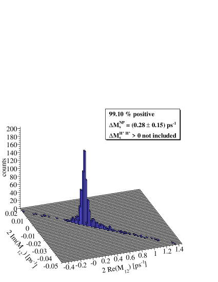
As a first check, we have verified that the phase of meson-antimeson oscillations in the MFV MSSM be aligned with the SM one. This feature is shown in Fig. 2 for the case. In the Figure, we have chosen a specific mass scenario for the SUSY scales and scanned the MFV parameters , , obtaining a distribution of values for . As expected, values are aligned along a line with slope .
In MFV, the phase of meson-antimeson oscillations is by definition not a good observable to search for NP effects. However, the same does not apply to the mass differences. As a matter of fact, by studying the latter, we found a number of interesting and sometimes surprising features, which we now discuss.
i. NP contributions are positive
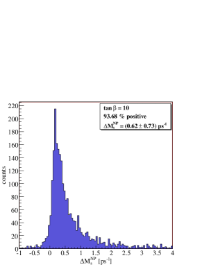
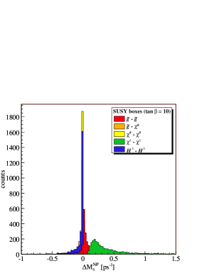
A first surprising fact emerges by studying the sum of the SUSY contributions to the meson mass differences. As already mentioned above, for every of the mass scenarios considered, we have randomly generated the MFV parameters , . The obtained distribution of values in translates into a corresponding distribution for the meson mass differences. As an example, one can look again at Fig. 2, displaying for the -meson. In this case, and an excellent estimate of is provided by the projection of the distribution along the . In the left panels of Figs. 3 to 6 we show how the distribution in looks like in four representative scenarios.999In the plots, the number of ‘events’ obtained after scanning , is set to 1000. We have verified that the distributions are left qualitatively unchanged when considering subsets of these 1000 points and when changing the binning, so that 1000 is a statistically significant number.
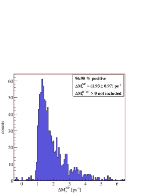
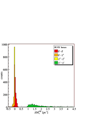
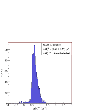
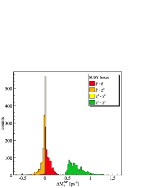
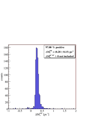
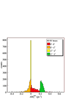
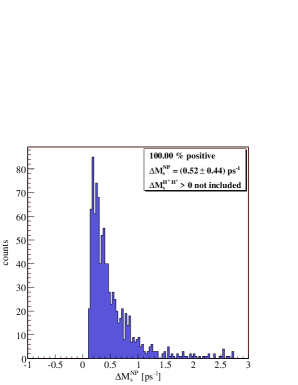
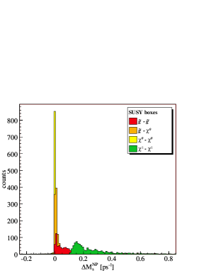
As one can immediately realize, almost the totality of points features , i.e. SUSY contributions to in the MFV MSSM at low are positive. We explicitly mention that in Fig. 2, as well as in Figures 3-6 below, charged Higgs boxes are not included. Their contribution amounts to a further positive shift of the distribution representing the sum of the other contributions, since Higgs boxes do not depend on the MFV parameters .
In the following discussion, we will get further insight on the positiveness of the SUSY corrections to meson mixings, by analyzing the separate SUSY contributions which sum up to give . Their interplay and a number of additional checks turn out to provide as many arguments in support of the above statement.
ii. Mass regimes
The positiveness of the sum of SUSY contributions holds true, irrespective of the mass scenario chosen. As a matter of fact, the 48 scenarios we have considered turn out to be classifiable into 4 main ‘mass regimes’, each characterized by a definite interplay among the various SUSY contributions. The deciding factors are the choice of the generic squark mass and of the magnitude of , the rest of the mass parameters, as well as the sign of , playing only a minor role once these are fixed. Specifically, one can choose a ‘not large’ value for the generic squark scale (i.e. GeV in our eq. (48)) and (A) small or (B) intermediate or (C) large. Alternatively, there is one more mass regime (D) when one chooses a large value for , irrespective of the choice of all the other SUSY scales, including . The four scenarios displayed in Figs. 3 to 6 are representative of such mass regimes, in the order (A) to (D).
iii. Interplay between chargino and gluino boxes
Let us now have a closer look into the various mass regimes, by discussing, within each of them, the main features of the separate contributions. The latter are displayed in the right panels of Figs. 3 to 6. As one can see from the figures – and as it will emerge from the subsequent discussion – the main actors in determining the sum of SUSY contributions to meson oscillations are chargino and gluino boxes, the remaining ones playing a minor role. We remind the reader that Higgs contributions are not considered in this discussion and not included in Figs. 3 to 6. For low , Higgs contributions trivially amount to a positive shift of the total result. We will address this point in a specific section.
Mass regime (A). Here, the smallness of implies a low value for the lightest
chargino mass eigenstate (see eq. (35)). As a consequence, contributions from
charginos tend to be large, of the order of ps-1. In addition they are positive,
being dominated by the SM operator [6]. Gluino contributions
are negligible in this scenario, and the reason, still related with the smallness of ,
will be clear from the discussion in mass regime (C) below.
A decrease in only reinforces the chargino dominance. One finds in this case that
gluino boxes remain negligible, while, for chargino ones, the up-squark mass scale gets
lower and their contribution is correspondingly increased. As a matter of fact,
Fig. 3 shows somehow the ‘worst’ case among the low ones within
our studied scenarios. In the other cases, the chargino dominance is even more evident
and the number of points with even closer to %.
Mass regime (B), with moderate, is a case of transition, intended to show the rate of decrease in importance of chargino contributions with increasing . Chargino contributions are still dominant as compared to gluino ones. Hence, in this respect, the situation is not qualitatively different from regime (A). On the whole, an increase in from to GeV corresponds to a decrease in the total signal from to ps-1, and similarly to regime (A), the total signal drops abruptly beneath the peak value.
Mass regime (C) occurs then for large . In this case, the flavour diagonal LR
entries in the down-squark mass matrix are large (see eq. (17)) and in connection with
the flavour mixing induced by LL entries, enhance contributions from scalar operators in
gluino boxes. Even if the up-squark mass matrix has in principle the same structure, the
same mechanism turns out to be not efficient in enhancing chargino
scalar contributions.101010One can provide an intuitive argument for this fact as follows:
gluino contributions to the various operators have the structure
, with defined in eq.
(22). Such structure holds for every operator. On the other hand, chargino
contributions to scalar operators have the structure , with the left (right) chargino-up squark-down quark
vertex coupling (see Appendix), while a similar structure – but with four
vertices – holds for the contributions to . Now, since and
(see Appendix A.2), in the case of charginos,
contributions other than are always made small by a suppression factor of .
The main parametric dependence ruling the above mechanism for gluino contributions is then
the product (see eq. (17)). One should also note that
the increase in the value of with respect to the previous regimes largely
suppresses chargino contributions, helping in turn chargino and gluino boxes to become
of comparable size.
The right panel of Fig. 5 displays a typical case for mass regime (C),
with gluino contributions amounting to roughly % positive corrections to the
chargino signal. We note here the occurrence of another interesting mechanism: in cases
where the squark scale and/or the mass are small (as in the example of
Fig. 5), gluino-neutralino boxes give a negative and relatively
important contribution. However, the latter is typically outpaced by the positive
contribution from pure gluino boxes (plus of course that from charginos), with a total
signal around ps-1. A similar mechanism can already be recognized in regime
(B) (see Fig. 4), but in that case is less evident.
We mention that, within the set of scenarios corresponding to regime (C), we found ‘extreme’
cases where scalar contributions from gluino boxes completely overwhelm any other contribution.
These occur when choosing a very light squark scale, GeV. In these cases, chargino
boxes amount to a small positive signal, while gluino-neutralino boxes give a contribution which
is negative and relatively large. The latter is again significantly counterbalanced by the positive, large
signal from gluinos and the sum of contributions results in a positive, quite spread signal for
. However, such extreme cases correspond to very light squark masses, the lightest
down- and up-squarks being around and GeV, respectively, which is very
unrealistic.111111As a further remark, we note that choosing large, with small,
causes the squark mass matrices’ determinants to be negative for most of the parameter space in the
MFV parameters , implying in turn an odd number of negative mass squared
eigenvalues. The corresponding point in the parameter space is then discarded as unphysical. As
a matter of fact, for GeV and GeV, the ratio of discarded to
valid points is , but this number drops to already for GeV.
Mass regime (D) is characterized by a large value for the squark scale , in our case GeV, and basically unaffected by the choice of any other parameter. In this case, the largeness of the squark scale sets to zero gluino-neutralino contributions, whose negative skewness had some effect in the previous cases. On the other hand, both chargino and gluino distributions (positive) are characterized by a long tail, as shown on the right panel of Fig. 6. The respective contributions are comparable in size, with the magnitude of those from gluinos growing with . The average SUSY signal is generically small, ps-1.
As a last overall remark, we explicitly note that, in all regimes considered, the magnitude of contributions coming from the flavour off-diagonal elements in the down-squark matrix, entering gluino and neutralino boxes, typically does not exceed ps-1. Therefore the latter set of contributions is strictly important only when also chargino contributions are small, i.e. in regimes (C) and in particular (D). We may add that such regimes are phenomenologically relevant after the simple observation that the experimental measurement of oscillations [17] and its agreement with the SM central value undoubtedly favour small NP corrections with respect to large ones. The final word will be provided by a substantial decrease of the lattice error, to the level of a few percent.
iv. Role of charged Higgs boxes
In the above study, we have completely omitted the inclusion of charged Higgs boxes. Recalling the discussion at the end of Section 4, we can now investigate their contribution separately, as a function of the single new SUSY scale they introduce, namely the physical charged Higgs mass .
In Fig. 7 we report the charged Higgs contribution to as a function of , for values of between and . The hatched area on the left of GeV represents the region excluded after direct experimental searches [18].
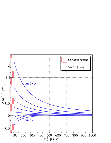
As one can see, for charged Higgs boxes give a positive correction to , irrespective of the value assumed by the physical mass . For this reason, we have chosen not to include such correction in the previous study on our mass scenarios: for each of them, Higgs contributions amount to a constant, positive shift of the final result. Then, in particular, the plots of Figs. 3-6 provide only a ‘lower bound’ on , to be augmented by the contribution from Higgs boxes.
It is interesting to give instead an indicative upper bound on the MFV MSSM contributions to for low . To this aim, we can consider mass regime (A) – chargino dominated – which tends to give the largest positive corrections (around ps-1, see Fig. 3), together with Higgs contributions taken at a small value for GeV. By looking at Fig. 7, one can see that Higgs corrections amount to roughly another ps-1. So, one can estimate MFV MSSM corrections to not to exceed ps-1. However, they are typically considerably smaller than this upper bound, as one can see by inspection of the various mass regimes (see also Fig. 8 below). This fact shows, for the case of mixing, that explicit implementation of the MFV limit in the MSSM leads to a naturally small correction to the SM prediction: in fact, expansions (19) analytically realize the condition of “naturalness of near flavour conservation” advocated in [12].
v. The case of
We applied the entire strategy described above also to the case of . Results are completely analogous, so we will limit to a few observations.
Keeping for the moment aside charged Higgs contributions, the magnitude of SUSY corrections , normalized to the SM prediction , is basically the same as the corresponding quantity in the case, in all our studied scenarios. Also the shapes of the distributions of values for the single contributions look very similar in the and cases.
This leads to the following remark. Even in scenarios where gluinos give important contributions from scalar operators, the latter do not bring about a sensible dependence on the external quark flavours. In fact, leading scalar contributions go as , and those in or respectively are subleading ones. The effect of the latter is moreover completely hidden, in our case, by the lack of knowledge of the SUSY scales and of the MFV parameters.
The inclusion of charged Higgs contributions does instead ‘distinguish’ the case of with respect to that of . Now contributions to the LR scalar operator behave as for (look at the coefficient in the Appendix).121212At the same time, contributions to are suppressed by . For , however, effects on the ratio are within %. Only for do they become larger than %, and can be visible once the lattice error on is at least halved with respect to the present value.
6 Additional MonteCarlo’s and role of
In this Section we elaborate on our main findings, as described in the previous study. In particular, we provide further arguments in support of our results, by verifying them with a set of additional numerical studies. The latter are designed to explore possible loopholes in the above treatment, and to address the question how the picture changes when increasing from strictly low values.
From the above discussion, it is evident that the positiveness of the SUSY correction in the MFV MSSM is due to an interplay among different contributions, the most important being those from charginos and gluinos. In addition, for , Higgs boxes further shift the result by a positive amount, depending on the chosen .
Such findings followed from a MonteCarlo study in which SUSY masses were fixed and MFV parameters generated with flat distributions. To check for the robustness of our results, we also performed additional MonteCarlo’s.
Random scan of both SUSY scales and MFV parameters
In a first alternative set of runs, we scanned both SUSY scales and MFV parameters. In particular SUSY masses were assumed to follow flat distributions in the range GeV.131313The lower bounds for and for were set to GeV and GeV, respectively. In such runs, we also set to different values in the range . This allowed us to study the resulting modifications in the various contributions, in particular in those from Higgs boxes, which for a light tend to be negative when .
The results of such global runs are reported in Fig. 8 for the cases of and .
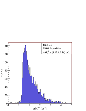
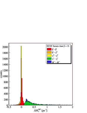
As the Figure shows, for the positiveness of the sum of results is confirmed by the global run as well.141414We mention that a further verification was carried out by varying the ‘B-parameters’ for the effective operator matrix elements within the ranges allowed in [23]. Neither the positiveness of the sum of the results, nor the interplay beween charginos and gluinos, resulting in the above regimes (A),…,(D), are touched at all by variations of the B-parameters. The right panel of the first row also shows that, if is assumed to be flatly distributed in the range GeV, then Higgs contributions tend to give a distribution completely analogous to that for charginos (the latter hides almost entirely the former in the plot).
The second row of Fig. 8 reports then the same distributions, when . As one can see, contributions from charginos, gluinos, neutralinos and mixed gluino-neutralino are left qualitatively unchanged by the variation in . On the other hand, Higgs contributions are very small and negative, as expected also from the lowermost curve in Fig. 7. However, this fact has quite a small impact on the sum of all the results, which remains chiefly positive (see left panel). We mention that a further increase in to confirms a similar picture: all contributions but for Higgs boxes build up an almost totally positive distribution. The negativity of Higgs boxes, however, starts to matter, and the sum of all contributions is positive in roughly % of the counts.
Changing the ranges for MFV parameters
A second set of runs was devised to check for possible variations in our findings, when the MFV parameters defining the expansions (19) are varied in ranges different from those specified in eq. (54). In the latter, the choice of as the upper bound is dictated by various considerations. First, on ‘aesthetical’ grounds, such bound should be realistic, if the MFV expansion of the soft terms as functions of the Yukawa couplings is a ‘natural’ one. The interpretation is that and ‘couplings’ of O(1) cause the new flavour violating effects originated by the soft terms to be at the same time CKM-like – i.e. generated by the SM Yukawa couplings, according to the very MFV paradigm – and natural [12, 1]. Second, on more technical grounds, enlarging too much the range of variation for the and may lead to a non-efficient exploration of the full parameter space allowed. However, on this latter point, we have verified that the shape of the distributions remains stable already after a few hundreds random values for the .
In this second MonteCarlo study, we kept SUSY masses fixed to scenarios, as described in Section 5.1, and increased the upper bounds for the MFV parameters from to . The main effect of increasing the ranges of variability is to ‘smoothen’ the difference between chargino and gluino distributions in the various scenarios and consequently to make regimes (A),…, (D) more similar to one another. However, the main features of each of them, as well as the positiveness of the sum of contributions, are left unchanged.
On the whole, a choice of the MFV parameters according to the ranges (54) – mainly dictated by ‘naturalness’ – allows a better understanding of the interplay between chargino and gluino contributions in the different scenarios. It would be interesting to adopt a top-down approach to the determination of the MFV parameters , by considering e.g. SUSY Grand Unified Theories (GUT) which at low energy reproduce the soft SUSY breaking structure of the MSSM. If such SUSY GUTs can be constructed to be minimal flavour violating [33], then the at the EW breaking scale can be fitted by introducing the corresponding constraints (19) between soft terms and Yukawa couplings. The latter are both predicted within such models, in terms of the initial conditions at the GUT scale and of the running.
We conclude this section by stressing that the feature of positiveness for the sum of SUSY contributions to in the MFV MSSM is a precise signature of low . It is interesting to address the question whether a similar signature, but with sign reversed, applies to the MFV MSSM in the large limit. This regime requires however consideration of an additional set of contributions, represented by the double neutral Higgs penguins [8, 34, 9, 10, 35]. This goes beyond the scope of the present paper. For an comprehensive related study in the context of grand unification, see Ref. [36].
7 Various considerations on MFV
The concrete application of the MFV limit to a calculable NP model, like the MSSM, gives us now the opportunity to emphasize the main differences between the model independent approach of [1] and the former, phenomenological definition of MFV by [2]. We will also try and understand in which, among our studied scenarios for the SUSY scales, MFV contributions to meson oscillations are dominated by , the operator already present within the SM. This case is referred to as ‘constrained’ MFV (CMFV) [5] and its study will allow us to understand how natural CMFV is within the MSSM.
7.1 MFV: definition [1] versus [2]
According to the definition of MFV by [1], all the flavour and CP violation at the EW scale is generated by the Yukawa couplings present in the SM. As we stressed several times above, this does not mean that new sources of flavour violation should be set to zero, but instead that they should be taken as functions of the SM Yukawa couplings. The functional dependence is in turn fixed by their formal transformation properties under the flavour group and gives rise to expansions like (19).
On the other hand, the phenomenological definition of MFV by [2] does not start from the SM Yukawa couplings, but from the CKM matrix. In this approach, a theory is considered minimal flavour violating, when only interactions which display explicit proportionality to the CKM matrix are active. In this context, new sources of flavour violation are simply not considered, since they have a priori “nothing to do” with the CKM matrix.
However, in the more general approach by [1], the CKM matrix becomes a by-product of the SM Yukawa couplings. Then the possibility of treating the Yukawa couplings as spurion fields, allows to classify in terms of them any new source of flavour violation, and this is why the definition by [1] has a completely general applicability. As a matter of fact, it also provides a framework for systematic routes to beyond-MFV (see [37]).
In the general context of [1], let us finally establish a contact with definition [2]. Since in the approach [2] new flavour violating structures are taken as unrelated to the SM Yukawa couplings, it is clear that one can reach this definition by setting the MFV parameters , in expansions (19). In this respect, an interesting MFV study where effects beyond the less general framework [2] are not visible has been reported in Ref. [38]. Specifically, in this case squark flavor mixing effects proportional to Yukawa couplings are negligible (in particular there are no gluino contributions) and the coefficients are consistently set to zero.
7.2 Deviations from ‘constrained’ MFV
In this Section, we finally study – in the context of the Hamiltonian – the special case in which MFV MSSM contributions are dominated by the operator , the one already present in the SM. This case corresponds to ‘constrained’ MFV (CMFV) [5]151515For the sake of clarity, we mention that the definition of MFV adopted in [5] complies with [2].. We would like to stress that CMFV is a phenomenologically relevant limit: in fact, if MFV is motivated by the observation that experiments do not require new sources of flavour violation besides the SM Yukawa couplings, the constrained version of it is analogously justified by the fact that there is no compelling experimental evidence for contributions of effective operators other than the SM ones.
The latter statement is actually strictly true when one supposes that new effective operators be “strongly coupled”, i.e. multiplied by an overall ‘coupling’ factor taken to be (or ) [39, 1]. Bounds on new operator contributions are considerably alleviated, or removed altogether, when such operators are weakly coupled, as is typically the case for SUSY contributions to the observables considered in the bounds.
The limit of CMFV is a useful benchmark case to consider, both because of the generic argument on new operators mentioned above and because it is a very well satisfied feature of chargino contributions, which represent an important and sometimes dominating ingredient in the various mass regimes of MFV. In the present Section, we start again from our calculated MFV MSSM contributions to meson oscillations. We then compare – in the different mass scenarios considered – the part of the contributions which bears proportionality to with the rest of the contributions, due to operators besides the SM one. This exercise will allow us to understand how ‘natural’ is CMFV within the MSSM.
As a first step, we can define the ratio as
| (56) |
where are the Wilson coefficients of the Hamiltonian (see eq. (47)) in the MFV MSSM. The ratio provides a good ‘quantitative’ understanding of the relative importance of contributions from non-SM operators with respect to , in the case.
Within every of the mass scenarios considered, the ratio is then a distribution of values depending on the MFV parameters . In Figs. 9-12 we report such distribution in the four representative regimes studied in Section 5.2. In particular, left panels display for the sum of all contributions, leaving aside, again, those from charged Higgs, on which we will comment separately. The percentage reported on top of the plots gives the number of counts satisfying . This bound can be considered – in our MFV MSSM case – a quantitative ‘definition’ of CMFV. According to it, a given estimate of is taken to be CMFV, if contributions from operators other than do not exceed % of the contribution from . We warn the reader that this upper bound (and the corresponding definition associated with it) has of course a large degree of arbitrariness: we chose % in view of the still large hadronic uncertainties associated with the estimate of the .
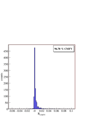
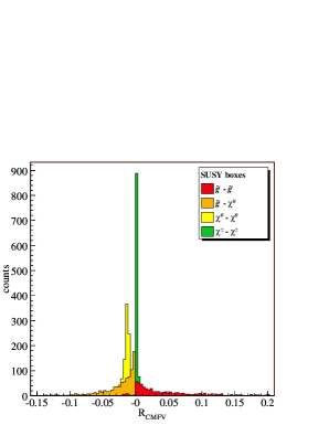
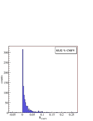
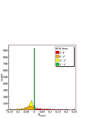
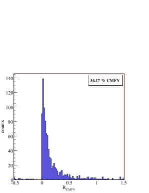
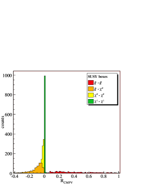
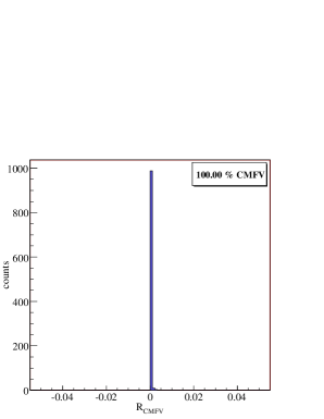
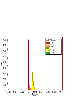
As one can see from the left panels of Figs. 9-12, mass regimes (A) and (D) satisfy well CMFV. Mass regimes (B) and in particular (C), on the other hand, do not.161616We mention that the case displayed in Fig. 10 is the one with the highest CMFV percentage among the studied scenarios belonging to mass regime (B). Further insight can be gained by looking at the right panels of the same Figures, where is displayed for the single contributions (in this case the ratio (56) was calculated by restricting separately to for gluino-gluino boxes, and so on for the other contributions). One immediately recognizes that regime (A) is -dominated, since chargino contributions are the most important ones. Gluinos are not CMFV, but they are unimportant. In regime (D), instead, charginos and gluinos are of the same size, but both -dominated. Finally, in regimes (B) and especially (C), CMFV does not apply: in fact, while charginos are always important and -dominated, gluinos are not negligible and not -dominated. As a matter of fact, for gluinos is in these cases very spread, typical values being in the range . We mention that such large values are not shown in the plots of Figs. 10 and 11.
Let us then address how the above picture is modified when adding contributions from charged Higgses. The for the latter, in the case of , ranges between and , for GeV and GeV respectively. However, contributions from scalar operators steadily increase in importance when increasing : for Higgs contributions are not CMFV if GeV and, already from , in the full range of masses considered for . Then, whether the total sum is CMFV or not, it depends on how large the contribution from Higgses is, with respect to the other contributions, i.e. on the Higgs mass chosen (see Fig. 7).
We remark at this point that an increase in importance of scalar contributions affects, in general, and in a different way. However, in the case of Higgs boxes, we found that the ratio of has a sensitivity with respect to variations of below %, when is strictly small. Variations start to be visible only from , when they become %. This point was already stated at the end of Section 5, when discussing the case of .
Concerning contributions other than charged Higgses, we note that large deviations from -dominated MFV apply when is not small – regimes (B) and (C) –. However, such deviations turn out not to affect and in a sensibly different way, so that their impact is not visible in the ratio . The reason was, again, already explained at the end of Section 5.
However, the above discussion allows us to place a warning message on the conventional wisdom that, for low , MFV in the Hamiltonian is -dominated. This is clearly not true when Higgs and gluino contributions are included, and when is not small in magnitude. In this case, the approximation , on the ground that is small, turns out not to work.
7.3 A lower bound on from CMFV
Recently, it has been shown analytically in [40] that, within the CMFV models, the lower bounds on are simply given by . The proof holds, assuming general exchange of charged gauge bosons, Goldstone bosons and physical scalars in boxes together with Dirac fermions, and under phenomenologically realistic assumptions on their masses. On the other hand, two possible exceptions to the argument were found to arise in the presence of Majorana fermions and of neutral gauge bosons in box diagrams, which could individually bring below . Within the model-independent approach of [40], it seems impossible to exclude CMFV models involving negative contributions to , caused by Majorana fermions and/or neutral gauge bosons, that are not cancelled by the remaining positive contributions from the other possible particle exchanges.
Within our study, we found in the previous Section that only mass regimes (A) and (D) are -dominated, i.e. CMFV. In particular, the above mentioned exception, of a CMFV case in which Majorana fermion contributions are not negligible, arises in regime (D) (see Fig. 6). However in this case, Majorana contributions, represented by the gluino boxes, are also positive, so that, at least for low , the lower bounds of [40] still hold. Finally, regime (A) exactly corresponds to the assumptions made in the proof of [40], since Majorana contributions are negligible. In this case we numerically confirm the positivity of the NP contributions.
We find actually remarkable that, within the MFV MSSM at low , the condition holds even when new operators give non-negligible contributions.
8 MFV-Unitarity Triangle
In this Section, we would like to emphasize that the so-called Universal Unitarity Triangle (UUT) [2] is valid only within the CMFV models, and not within the general class of MFV models, like the MSSM considered here.
Indeed, the usual construction of the UUT is based on the value of the angle , measured by means of the asymmetry, and on the value of the side , obtained from the ratio , that within CMFV is independent of any new physics contributions.
As already stressed in [10, 5], in the context of the MSSM at large , the presence of new operator contributions to and generally modifies the relation between and , so that it now reads [10, 5]
| (57) |
with and being a known non-perturbative parameter, .
Basing on the results of the previous sections, formula (57) applies to the MSSM at low as well, with , due to the presence of new operators that differently affect and . This can already be seen by adding to the SM expression for the mass differences, the contributions from the charged Higgs boxes, which do not depend on the MFV parameters . As we showed in Section 7, when addressing deviations from CMFV, the ratio is subject to variations at the percent level, depending on the value chosen for . Similar effects occur in principle when considering the other contributions as well, but in this case the variation is completely hidden by the lack of knowledge of the values for the MFV parameters and of course of the SUSY scales. The departure from CMFV is more pronounced in the MFV MSSM for large , but such analysis is beyond the scope of the present paper.
The above argument clearly demonstrates that the MFV MSSM, even at low , does not belong to the class of CMFV models, and consequently, the UUT obtained from and is not generically valid in MFV.
This discussion suggests that the unitarity triangle valid for all MFV models is not the UUT of [2] – and analyzed in detail by [4] – but a triangle constructed from the angle and the new-physics-independent value of or from tree-level decays.
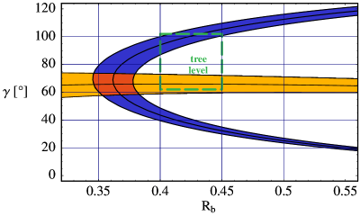
In this context, the known value establishes a correlation between the side ,
| (58) |
of the unitarity triangle and the angle , that is valid for all models with MFV. Such correlation is represented in Fig. 13 as a blue area, under the assumption . The orange area in the Figure displays instead the region characterized by fixed to the value in eq. (57), with and . The intersection between the two areas – displayed in red – is then the one allowed to CMFV. Fig. 13 also shows the -allowed range from tree-level decays, namely and , as a green dashed box. The latter overlaps with the higher branch of the MFV area but not with the CMFV one. This indicates, on the one hand, somehow a ‘tension’ [5] between the tree-level determination of and the one favoured by CMFV. On the other hand, the overlap between the green box and the blue area suggests that this tension disappears within MFV, provided .
It will be interesting to monitor with the help of Fig. 13 the progress in the determination of and of the angle from tree-level decays, and to verify whether the correlation in question is satisfied by the data.
Equivalently, with precise values of and , that are used for the construction of the reference unitarity triangle, it will be possible to find out whether the CMFV UUT or the MFV-UT is chosen by nature, or instead if one has to introduce non-MFV interactions to fit the data. This would occur if the experimental point lies outside the blue area in Fig. 13.
9 Conclusions and Outlook
In this paper, we have applied the effective field theory definition of Minimal Flavour Violation (MFV) to the MSSM and explicitly shown how, by this definition, the new sources of flavour and CP violation present in the MSSM become functions of the SM Yukawa couplings. We have subsequently applied the MFV limit to the MSSM Hamiltonian at low .
Our findings can be summarized in the following main messages:
-
1.
In the MFV limit of the MSSM, the soft breaking terms become functions of the SM Yukawa couplings. This non-trivial functional dependence causes flavour violation due to soft terms to be not zero in MFV, but instead ‘CKM-like’. The constraints imposed on the soft terms by the MFV assumption lead to a significant increase in the predictive power of the model.
-
2.
The supersymmetric corrections to at low are found to be always positive with respect to the SM formula. This feature is due to an interesting interplay between the chargino and gluino box diagram contributions.
-
3.
Even at low , the MSSM does not in general belong to the class of models with CMFV, in contrast to the statements made in the literature. The presence of gluino box diagram contributions necessarily brings in new operators beyond the one, whose importance depends on the mass regime chosen.
-
4.
The side , used in the determination of the Universal Unitarity Triangle, is actually not a good constant in MFV. Within the MFV MSSM at low , we have found variations that can reach the percent level, depending again on the mass regime chosen, and on the value of . To resolve such variations, one however needs a lattice determination for with an error at most half the present value. In the case of the MFV MSSM at large the situation is in this respect ‘easier’, since larger deviations from the CMFV value of are more likely.
-
5.
A unitarity triangle valid in all MFV models (MFV-UT) can be constructed using only or , from tree-level decays, and the angle , extracted from . In particular, with the measured value of , MFV implies a testable correlation between and . With the present high value of , MFV favours . The LHC program on the measurement of is then of utmost importance to cleanly consolidate – or disprove – the MFV paradigm.
Acknowledgments
A.J.B. would like to thank Gino Isidori for his critical remarks in connection with the bound [40], that strengthened the motivation to carry out this study. D.G is indebted to Gino Isidori for insightful conversations on the topic of MFV, that were precious for framing the subject of this work. The authors thank also Monika Blanke for a careful reading of the manuscript and useful comments. Thanks are also due to Uli Haisch and Federico Mescia for useful comments. This work has been supported in part by the Cluster of Excellence “Origin and Structure of the Universe” and by the German Bundesministerium für Bildung und Forschung under contract 05HT6WOA.
Appendix A Wilson coefficients for the effective Hamiltonian in the MSSM
A.1 Contributions
Below we list the non-vanishing new physics contributions to the Wilson coefficients for mixing, eq. (47). The case of mixing is obtained by the replacement (or where applicable) in the external quark indices. In the following expressions, it is always understood that internal indices are summed over their respective ranges, i.e. for quarks, for squarks, for charginos and for neutralinos.
Charged Higgs contributions
| (A.59) |
| (A.60) |
| (A.61) |
| (A.62) |
| (A.63) |
| (A.64) |
The above coefficients and arise from the sum of , and boxes (with the charged Goldstone boson, entering calculations away from the unitary gauge).
Chargino contributions
The coefficients and can be obtained from and respectively by the replacement of left- and right-handed chargino couplings .
Neutralino contributions
| (A.65) |
| (A.66) |
| (A.67) |
| (A.68) |
Interchanging left- with right-handed neutralino couplings in yields the expressions for the Wilson coefficients .
Mixed neutralino and gluino contributions
| (A.69) |
| (A.70) |
| (A.71) |
| (A.72) |
| (A.73) |
To obtain the coefficients from , one again has to interchange left- with right-handed neutralino couplings. In addition, analogous replacements have to be performed for the elements of the down squark mixing matrix that explicitly appear in the above expressions: and .
Gluino contributions
| (A.74) |
| (A.75) |
| (A.76) |
To get the corresponding expressions for the coefficients one again has to carry out the following replacements for the down squark mixing matrix: and .
A.2 Chargino and Neutralino couplings
Here we explicitly report – in terms of gauge couplings, Yukawa couplings and rotation matrices – the chargino and neutralino couplings used in the expressions for the Wilson coefficients.
A.3 Loop functions
Finally, we give the explicit expressions for the loop functions that appear in the Wilson coefficients listed above.
| (A.77) |
| (A.78) |
References
- [1] G. D’Ambrosio, G. F. Giudice, G. Isidori, and A. Strumia, Minimal flavour violation: An effective field theory approach, Nucl. Phys. B645 (2002) 155–187, [hep-ph/0207036].
- [2] A. J. Buras, P. Gambino, M. Gorbahn, S. Jager, and L. Silvestrini, Universal unitarity triangle and physics beyond the Standard Model, Phys. Lett. B500 (2001) 161–167, [hep-ph/0007085].
- [3] A. J. Buras, Minimal flavor violation, Acta Phys. Polon. B34 (2003) 5615–5668, [hep-ph/0310208]. Lectures given at 43rd Cracow School of Theoretical Physics, Zakopane, Poland, 30 May - 9 Jun 2003.
- [4] See UTfit website: http://www.utfit.org.
- [5] M. Blanke, A. J. Buras, D. Guadagnoli, and C. Tarantino, Minimal flavour violation waiting for precise measurements of , , , , and , JHEP 10 (2006) 003, [hep-ph/0604057].
- [6] E. Gabrielli and G. F. Giudice, Supersymmetric corrections to at the leading order in QCD and QED, Nucl. Phys. B433 (1995) 3–25, [hep-lat/9407029].
- [7] A. J. Buras, P. Gambino, M. Gorbahn, S. Jager, and L. Silvestrini, and rare and decays in the MSSM, Nucl. Phys. B592 (2001) 55–91, [hep-ph/0007313].
- [8] A. J. Buras, P. H. Chankowski, J. Rosiek, and L. Slawianowska, , and the angle in the presence of new operators, Nucl. Phys. B619 (2001) 434–466, [hep-ph/0107048].
- [9] A. J. Buras, P. H. Chankowski, J. Rosiek, and L. Slawianowska, Correlation between and in supersymmetry at large , Phys. Lett. B546 (2002) 96–107, [hep-ph/0207241].
- [10] A. J. Buras, P. H. Chankowski, J. Rosiek, and L. Slawianowska, , and in supersymmetry at large , Nucl. Phys. B659 (2003) 3, [hep-ph/0210145].
- [11] R. S. Chivukula and H. Georgi, Composite technicolor Standard Model, Phys. Lett. B188 (1987) 99.
- [12] L. J. Hall and L. Randall, Weak scale effective supersymmetry, Phys. Rev. Lett. 65 (1990) 2939–2942.
- [13] J. Rosiek, Complete set of Feynman rules for the Minimal Supersymmetric extension of the Standard Model, Phys. Rev. D41 (1990) 3464. Erratum [hep-ph/9511250].
- [14] R. D. Peccei and H. R. Quinn, Constraints Imposed by CP Conservation in the Presence of Instantons, Phys. Rev. D16 (1977) 1791–1797.
- [15] L. J. Hall, V. A. Kostelecky, and S. Raby, New flavor violations in supergravity models, Nucl. Phys. B267 (1986) 415.
- [16] F. Gabbiani, E. Gabrielli, A. Masiero, and L. Silvestrini, A complete analysis of FCNC and CP constraints in general SUSY extensions of the standard model, Nucl. Phys. B477 (1996) 321–352, [hep-ph/9604387].
- [17] CDF Collaboration, A. Abulencia et al., Observation of oscillations, Phys. Rev. Lett. 97 (2006) 242003, [hep-ex/0609040].
- [18] W.-M. Yao et al., Review of Particle Physics, Journal of Physics G 33 (2006) 1+.
- [19] CDF Collaboration, A. A. Affolder et al., Search for gluinos and scalar quarks in collisions at TeV using the missing energy plus multijets signature, Phys. Rev. Lett. 88 (2002) 041801, [hep-ex/0106001].
- [20] DØ Collaboration, V. M. Abazov et al., Search for squarks and gluinos in events with jets and missing transverse energy in collisions at = 1.96-TeV, Phys. Lett. B638 (2006) 119–127, [hep-ex/0604029].
- [21] G. Isidori and P. Paradisi, Hints of large in flavour physics, Phys. Lett. B639 (2006) 499–507, [hep-ph/0605012].
- [22] M. Ciuchini, G. Degrassi, P. Gambino, and G. F. Giudice, Next-to-leading QCD corrections to in supersymmetry, Nucl. Phys. B534 (1998) 3–20, [hep-ph/9806308].
- [23] D. Becirevic, V. Gimenez, G. Martinelli, M. Papinutto, and J. Reyes, B-parameters of the complete set of matrix elements of operators from the lattice, JHEP 04 (2002) 025, [hep-lat/0110091].
- [24] C. R. Allton et al., B-parameters for supersymmetric operators, Phys. Lett. B453 (1999) 30–39, [hep-lat/9806016].
- [25] JLQCD Collaboration, S. Aoki et al., mixing in quenched lattice QCD, Phys. Rev. D67 (2003) 014506, [hep-lat/0208038].
- [26] UKQCD Collaboration, L. Lellouch and C. J. D. Lin, Standard model matrix elements for neutral B meson mixing and associated decay constants, Phys. Rev. D64 (2001) 094501, [hep-ph/0011086].
- [27] JLQCD Collaboration, N. Yamada et al., B meson B-parameters and the decay constant in two-flavor dynamical QCD, Nucl. Phys. Proc. Suppl. 106 (2002) 397–399, [hep-lat/0110087].
- [28] JLQCD Collaboration, S. Aoki et al., mixing in unquenched lattice QCD, Phys. Rev. Lett. 91 (2003) 212001, [hep-ph/0307039].
- [29] E. Dalgic et al., mixing parameters from unquenched lattice QCD, hep-lat/0610104.
- [30] M. Ciuchini et al., Next-to-leading order QCD corrections to effective Hamiltonians, Nucl. Phys. B523 (1998) 501–525, [hep-ph/9711402].
- [31] A. J. Buras, M. Misiak, and J. Urban, Two-loop QCD anomalous dimensions of flavour-changing four- quark operators within and beyond the standard model, Nucl. Phys. B586 (2000) 397–426, [hep-ph/0005183].
- [32] A. J. Buras, Weak Hamiltonian, CP violation and rare decays, hep-ph/9806471. Published in *Les Houches 1997, Probing the Standard Model of particle interactions, Pt. 1* 281-539.
- [33] B. Grinstein, V. Cirigliano, G. Isidori, and M. B. Wise, Grand unification and the principle of minimal flavor violation, Nucl. Phys. B763 (2007) 35–48, [hep-ph/0608123].
- [34] G. Isidori and A. Retico, Scalar flavour-changing neutral currents in the large- limit, JHEP 11 (2001) 001, [hep-ph/0110121].
- [35] A. Freitas, E. Gasser, and U. Haisch, Supersymmetric large corrections to and revisited, hep-ph/0702267.
- [36] E. Lunghi, W. Porod, and O. Vives, Analysis of enhanced corrections in MFV GUT scenarios, Phys. Rev. D74 (2006) 075003, [hep-ph/0605177].
- [37] T. Feldmann and T. Mannel, Minimal Flavour Violation and Beyond, JHEP 02 (2007) 067, [hep-ph/0611095].
- [38] G. Isidori, F. Mescia, P. Paradisi, C. Smith, and S. Trine, Exploring the flavour structure of the MSSM with rare K decays, JHEP 08 (2006) 064, [hep-ph/0604074].
- [39] R. Barbieri and A. Strumia, The ’LEP paradox’, hep-ph/0007265.
- [40] M. Blanke and A. J. Buras, Lower bounds on from constrained minimal flavour violation, hep-ph/0610037.