Total cross-section at LHC from minijets and soft gluon resummation in the infrared region

Abstract

A model for total cross-sections incorporating QCD jet cross-sections and soft gluon resummation is described and compared with present data on $pp$ and ${\bar{p}}p$ cross-sections. Predictions for LHC are presented for different parameter sets. It is shown that they differ according to the small x-behaviour of available parton density functions.

12.38.-t;12.40.Nn;13.60.Hb;13.85.Lg

1 Introduction

The upcoming measurements at LHC are renewing considerable interest regarding predictions for total cross-sections. The model [1, 2] we shall describe in the following, attempts to link the rate with which total cross-sections rise, to the infrared behaviour of the strong coupling constant $\alpha_{s}$ and to QCD hard parton-parton scattering, using known phenomenological entities such as the available QCD parton density functions (PDFs).

2 The model

The energy behaviour of the total cross-section exhibits the following properties [3]

• an initial decrease

• a sharp change in curvature occurring somewhere between 20 and 50 GeV in the c.m. of the scattering hadrons

• a smooth rise which asymptotically follows a $\ln s$ or $\ln^{2}{s}$ type increase in consonance with the Froissart bound [4, 5]

The model we use is based on

1. hard component of scattering responsible for the rise of the total cross-section [6, 7]

2. soft gluon emission from scattering particles which softens the rise [1]

3. eikonal transformation which implies multiple scattering and requires impact parameter distributions inside scattering particles and basic scattering cross-sections [8]

According to our model, soft gluon emission is responsible for the initial decrease in $pp$, as well as for the transformation of the sharp rise due to the increase in gluon-gluon interactions into a smooth behavior. Thus soft gluon emission plays a crucial role, with care taken to extend resummation to the zero energy modes, in complete analogy for what is required by the Bloch-Nordsieck theorem for QED[9]. The model can then be referred to as the BN model, for reasons which will also be clearer in the following.

2.1 Details of the BN model

We use the following eikonal expression for the total inelastic cross-section:

$$\sigma_{inel}=\int d^{2}{\vec{b}}[1-e^{-n(b,s)}]$$ (1)

where $n(b,s)$ corresponds to the average number of inelastic collisions at any given value of the impact parameter b. Neglecting the real part of the eikonal, we then calculate the total cross-section as

$$\sigma_{total}=2\int d^{2}{\vec{b}}[1-e^{-n(b,s)/2}]$$ (2)

In our model $n(b,s)$ is split as

$$n(b,s)=n_{soft}(b,s)+n_{hard}(b,s)$$ (3)

where we postulate the following factorization

$$n_{soft/hard}(b,s)=A_{BN}^{soft/hard}(b,s)\sigma_{soft/hard}(s)$$ (4)

with

$$A_{BN}(b,s)=N\int d^{2}K_{\perp}\ e^{-iK_{\perp}\cdot b}{{d^{2}P(K_{\perp})}\over{d^{2}K_{\perp}}}$$ (5)

where N is a normalization factor such that $\int d^{2}{\vec{b}}A(b)=1$ and

$${{d^{2}P(K_{\perp})}\over{d^{2}K_{\perp}}}={{1}\over{(2\pi)^{2}}}\int d^{2}{\vec{b}}\ e^{iK_{\perp}\cdot b-\int_{0}^{q_{max}}d^{3}{\bar{n}}(k)[1-e^{-ik_{t}\cdot b}]}$$ (6)

is the transverse momentum distribution of initial state soft gluons emitted in the parton-parton collisions and where, for simplicity, $k_{\perp}\cdot b={\vec{k}}_{\perp}\cdot{\vec{b}}$. In Equation (6) $q_{max}$ is the maximum transverse momentum allowed by kinematics to single soft gluon emission in a given hard collision, averaged over the parton densities. According to the basic ansatz of the Eikonal Minijet Model (EMM),

$$\sigma_{hard}\equiv\sigma^{AB}_{\rm jet}(s)=\int_{p_{tmin}}^{\sqrt{s/2}}dp_{t}\int_{4p_{t}^{2}/s}^{1}dx_{1}\int_{4p_{t}^{2}/(x_{1}s)}^{1}dx_{2}\sum_{i,j,k,l}f_{i|A}(x_{1})f_{j|B}(x_{2})~{}~{}\frac{d\hat{\sigma}_{ij}^{kl}(\hat{s})}{dp_{t}}.$$ (7)

Here $A$ and $B$ denote particles ($\gamma,\ p,\dots$), $i,\ j,\ k,\ l$ are parton types and $x_{1},x_{2}$ the fractions of the parent particle momentum carried by the parton. $\hat{s}=x_{1}x_{2}s$ and $\hat{\sigma}$ are hard parton scattering cross–sections. As discussed in [1], kinematical considerations suggest [10]

$$q_{max}(s)={{\sqrt{s}}\over{2}}{{\sum_{i,j}\int{{dx_{1}}\over{x_{1}}}f_{i|A}(x_{1})\int{{dx_{2}}\over{x_{2}}}f_{j|B}(x_{2})\sqrt{x_{1}x_{2}}\int_{z_{min}}^{1}dz(1-z)}\over{\sum_{i,j}\int{dx_{1}\over x_{1}}f_{i|A}(x_{1})\int{{dx_{2}}\over{x_{2}}}f_{j|B}(x_{2})\int_{z_{min}}^{1}(dz)}}$$ (8)

with $z_{min}=4p_{tmin}^{2}/(sx_{1}x_{2})$ and $f_{i/a}$ the valence quark densities used in the jet cross-section calculation. The steps we follow to compare the model with data are then the following:

1. choose the parameters for the hard scattering part, namely

   (i) parton densities (PDF), $p_{tmin}$ and $\Lambda_{QCD}$ for the chosen PDF set in Equation (7)

   (ii) model for $\alpha_{s}$ in the infrared region and relevant parameters in Equation (6)

2. calculate $q_{max}(s,p_{tmin})$ for the given densities and $p_{tmin}$ using Equation (8)

3. calculate $n_{hard}(b,s)=A_{BN}^{hard}(b,s)\sigma_{jet}(s,p_{tmin})$

4. choose the parameters for the low energy part, namely

   (i) the constant low energy cross-section $\sigma_{0}$

   (ii) values for $q_{max}^{soft}$

5. calculate $n_{soft}(b,s)=A_{BN}^{soft}(b,s)\sigma_{0}(1+\epsilon{{2}\over{\sqrt{s}}})$ with $\epsilon=0,1$ depending upon the process being $pp$ or $p\bar{p}$

6. calculate $n(b,s)$ and thus $\sigma_{tot}$

7. choose the parameter set which gives the best description of the total cross-section up to the Tevatron data [11, 12, 13]

Notice that once a good set of parameters is found, one can use $n(b,s)$ with fitted parameters to calculate survival probabilities or diffractive Higgs production.

2.2 Application to total cross-section data

We show in this section the application of the model to the total cross-section for different PDFs. We find that our model is flexible enough to be able to reproduce the present data for $\sigma_{tot}$ using all presently available PDFs. In particular, all GRV [14, 15, 16] and MRST [17] densities give a good description using the singular $\alpha_{s}$ model described in [1], while CTEQ densities [18] give an acceptable fit up to Tevatron data, but then fail to rise further.

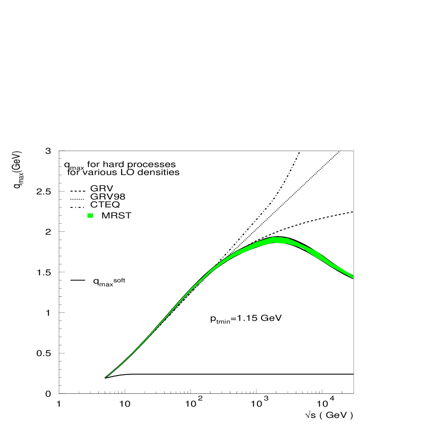
We present these results by following the previously listed steps. We start by choosing the parameters for the hard scattering, and, following our previous results [2], we fix $p_{tmin}=1.15\ GeV$ in the jet cross-sections and calculate $q_{max}$ for different PDF sets. We show the result in Fig.(1).

Figure 1: Average value of the maximum transverse momentum allowed to single gluon emission, according to the model in [2].

We notice the following:

• GRV densities are of two types, GRV98[16] for which $q_{max}$ keeps on increasing logarithmically and the older ones [14] for which $q_{max}$ slows down past the TeV region, albeit still slowly increasing

• CTEQ densities give values for $q_{max}$ which increase more rapidly than $\ln{s}$ after typical Tevatron energies

• MRST densities indicate a behaviour opposite to CTEQ, since they give $q_{max}$ values decreasing after the TeV cross mark.

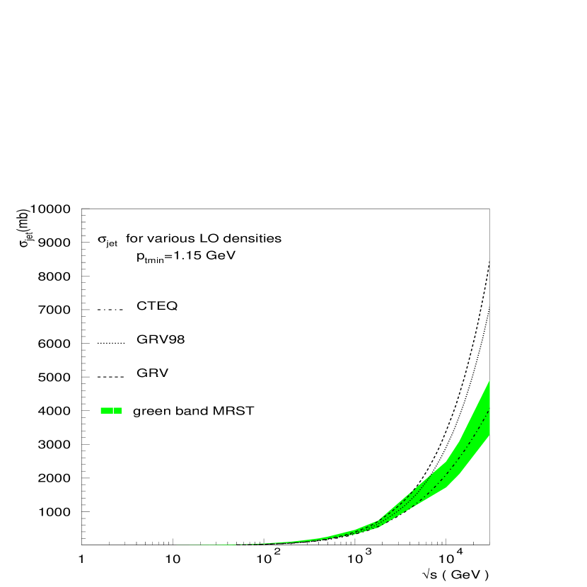
We now turn to the jet cross-sections and examine the growth with energy of $\sigma_{jet}$ for different PDFs. In Fig.(2) we plot these cross-sections for the same set of densities used to calculate $q_{max}$ and for $p_{tmin}=1.15\ GeV$.

Figure 2: Mini-jet QCD cross-sections for different PDFs as indicated in the figure

From this figure we notice that :

• the jet cross-sections for GRV densities increase faster than all the others

• the jet cross-sections for CTEQ increase more or less similarly to those for the MRST group

The implications are that $\sigma_{jet}$ with GRV densities, which increase faster than $\sigma_{jet}$ with MRST, need more softening, $\sigma_{jet}$ with CTEQ, which increase less than with GRV, should not be smeared that much.

To proceed further, we now need to calculate the $b-distribution$ and fix the low-energy parameters, like $\sigma_{0}$. The $b-distribution$ requires to input the behaviour of $\alpha_{s}$ in the infrared region. We have shown in [2] the need to use a singular but integrable expression for $\alpha_{s}$ in order to reproduce both the sudden rise and the subsequent softening of the total cross-section. Our choice is an expression like

$$\alpha_{s}(k_{t})={{12\pi}\over{(33-2N_{f})}}{{p}\over{\ln[1+p({{k_{t}}\over{\Lambda}})^{2p}]}}$$ (9)

which depends on the singularity parameter $p$, in addition to the scale $\Lambda$. In [2] we have chosen the value $p=0.75$ and $\Lambda=100\ MeV$, other choices are also possible [19]. Turning now to the low-energy part, $n_{soft}(b,s)$, we choose $\sigma_{0}=48\ mb$ and use for $A_{BN}^{soft}$ a set of $q_{max}$ values which reproduce the low energy behaviour, and which appear in Fig. (1).

3 Comparison with data and expectations at LHC densities

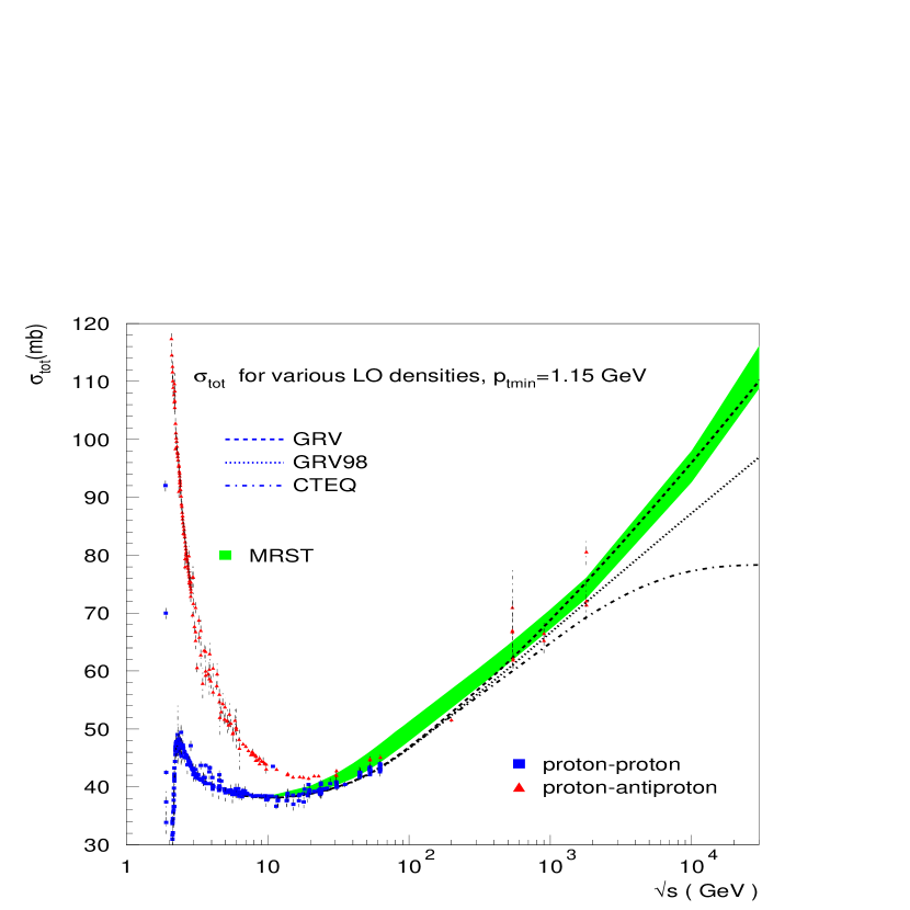
We can now input all the above in the eikonal representation for the total cross-section and obtain the results shown in Fig.(3)

Figure 3: Data for total cross-sections for $pp$ and $p{\bar{p}}$ compared with model predictions at LHC for $pp$ scattering, using different PDFs.

for the singular $\alpha_{s}$ case and GRV, MRST and CTEQ densities. For the sake of clarity, we only plot curves for $pp$ scattering, referring the reader to [2, 19] for the curves for $p{\bar{p}}$ and for a different parameter set, or for predictions from other models [5, 20, 21, 22, 23]. From the figure we see that the calculation with CTEQ densities appears very unlikely. The effect is due to the fact that the jet cross-sections in the CTEQ case do not rise as much as the others while the softening effect is stronger, as it is driven by $q_{max}$, which is strongly increasing for these densities. As a result, the cross-section starts decreasing. Notice that while the behaviour of $\sigma_{jet}$ is dominated by the gluon densities, that of $q_{max}$ is determined only by the valence quarks, as we assume this to be the leading order effect.

The curves shown in Fig.(3) indicate that the coming measurement at $\sqrt{s}=900\ GeV$ will be very important in determining which of these curves best describes the data. It can then be used to select the parameter set, basically PDF’s and $p_{tmin}$, for a prediction at the project LHC energy, $\sqrt{s}=14\ TeV$. If the UA5 [24] value at $\sqrt{s}=900\ GeV$ is confirmed with a comparable error, then, for the set of parameters discussed in this note, at $\sqrt{s}=14\ TeV$ our model gives $\sigma_{total}^{GRV98}=90.2\ mb$, $\sigma_{total}^{GRV}=100.2\ mb$ and $\sigma_{total}^{MRST76}=103.4\ mb$. As shown in [19], changing the parameter set, namely $\sigma_{0}$, $p_{tmin}$ or the singularity index $p$, give values in the range $88\div 111\ mb$.

4 Conclusions

We have presented a version of the eikonal minijet model which allows a good description of total cross-sections at asymptotic energies and discussed its connection with the small x-behaviour of various types of parton densities. This model is based on a softening of the mini-jet cross-sections due to an s-dependent b-distribution in the proton, which we calculate using a soft gluon resummation model down to zero energy of the soft gluons.

References

- [1] A. Corsetti, A. Grau, G. Pancheri and Y. N. Srivastava, Phys. Lett. B382, 282 (1996) [hep-ph/9605314]; A. Grau, G. Pancheri, and Y. N. Srivastava, Phys. Rev. D60 (1999) 114020, [hep-ph/9905228].
- [2] R. M. Godbole, A. Grau, G. Pancheri and Y. N. Srivastava, Phys. Rev. D72, 076001 (2005), [hep-ph/0408355].
- [3] Particle Data Group, J. Phys. G: Nucl. Part. Phys. 33 (2006) 1.
- [4] M. Froissart, Phys. Rev. 123 (1961) 1053.
- [5] M.M. Block, F. Halzen, Phys.Rev. D72 (2005) 036006, Erratum-ibid.D72 (2005) 039902, e-Print Archive: hep-ph/0506031
- [6] D. Cline, F. Halzen, and J. Luthe, Phys. Rev. Lett. 31 (1973) 491–494; T. K. Gaisser and F. Halzen, Phys. Rev. Lett. 54 (1985) 1754.
- [7] G. Pancheri and Y. N. Srivastava, Phys. Lett. B182 (1986) 199–207.
- [8] L. Durand and P. Hong, Phys. Rev. Lett. 58 (1987) 303.
- [9] F. Bloch and A. Nordsieck, Note on the Radiation Field of the Electron, Phys. Rev. 52 (1937) 54.
- [10] P. Chiappetta and M. Greco, Nucl. Phys. B199 (1982) 77.
- [11] N. Amos et. al., E710 Collaboration Phys. Rev. Lett. 68 (1992) 2433–2436.
- [12] F. Abe et. al., CDF Collaboration Phys. Rev. D50 (1994) 5550–5561.
- [13] C. Avila et. al., E811 Collaboration Phys. Lett. B445 (1999) 419–422.
- [14] M. Gluck, E. Reya, and A. Vogt, Z. Phys. C53 (1992) 127–134.
- [15] M. Gluck, E. Reya, and A. Vogt, Z. Phys. C67 (1995) 433–448.
- [16] M. Gluck, E. Reya, and A. Vogt, Eur. Phys. J. C 5 (1998) 461–470, [hep-ph/9806404].
- [17] A. D. Martin, R. G. Roberts, W. J. Stirling, and R. S. Thorne, Phys. Lett. B531 (2002) 216–224, [hep-ph/0201127].
- [18] H.L. Lai , J. Botts , J. Huston , J.G. Morfin , J.F. Owens , Jian-wei Qiu , W.K. Tung, H. Weerts, Phys.Rev.D51 4763-4782,1995. e-Print Archive: hep-ph/9410404CTEQ
- [19] R. M. Godbole, A. Grau, R. Hegde, G. Pancheri and Y. Srivastava, Pramana 66, 657 (2006), [hep-ph/0604214].
- [20] A. Donnachie and P. V. Landshoff, Phys. Lett. B296 (1992) 227–232, [hep-ph/9209205]; ibidem B595 (2004) 393–399,
- [21] M. M. Block, E. M. Gregores, F. Halzen and G. Pancheri, Phys. Rev. D D60, 054024 (1999) [hep-ph/9809403].
- [22] J. R. Cudell et. al.,, COMPETE Collaboration Phys. Rev. Lett. 89 (2002) 201801, [hep-ph/0206172]; J. R. Cudell et. al., [hep-ph/0212101].
- [23] E. G. S. Luna, A. F. Martini, M. J. Menon, A. Mihara and A. A. Natale, Phys. Rev. D72, 034019 (2005) [hep-ph/0507057]; R. F. Avila, E. G. S. Luna, and M. J. Menon, Phys. Rev. D67 (2003) 054020, [hep-ph/0212234].
- [24] G. J. Alner et al. (UA5 Collaboration), Z. Phys. C 32 (1986) 153.