KAIST-TH 2007/02

hep-ph/0703163


LHC Signature of Mirage Mediation
W.S. Cho1, Y.G. Kim1,2, K.Y. Lee,1, C.B. Park1 and Y. Shimizu1


1 Department of Physics, KAIST, Daejon 305–017, Korea

2 ARCSEC, Sejong University, Seoul 143-747, Korea


We study LHC phenomenology of mirage mediation scenario in which anomaly and modulus contributions to soft SUSY breaking terms are comparable to each other. A Monte Carlo study of mirage mediation, with model parameters α=1𝛼1\alpha=1,M0=500subscript𝑀0500~{}M_{0}=500 GeV, nM=1/2subscript𝑛𝑀12n_{M}=1/2, nH=1subscript𝑛𝐻1n_{H}=1 and tanβ=10tan𝛽10\rm{tan}\beta=10, is presented. It is shown that masses of supersymmetric particles can be measured in a model independent way, providing information on SUSY breaking sector. In particular, the mass ratio of gluino to the lightest neutralino for the benchmark scenario is determined to be 1.9mg~/mχ~103.1less-than-or-similar-to1.9subscript𝑚~𝑔subscript𝑚superscriptsubscript~𝜒10less-than-or-similar-to3.11.9\lesssim m_{\tilde{g}}/m_{\tilde{\chi}_{1}^{0}}\lesssim 3.1, well reproducing theoretical input value of mg~/mχ~102.5similar-to-or-equalssubscript𝑚~𝑔subscript𝑚superscriptsubscript~𝜒102.5m_{\tilde{g}}/m_{\tilde{\chi}_{1}^{0}}\simeq 2.5 which is quite distinctive from the predictions mg~/mχ~106greater-than-or-equivalent-tosubscript𝑚~𝑔subscript𝑚superscriptsubscript~𝜒106m_{\tilde{g}}/m_{\tilde{\chi}_{1}^{0}}\gtrsim 6 of other SUSY scenarios in which gaugino masses are unified at the GUT scale. The model parameters of mirage mediation can be also determined from various kinematic distributions.

1 Introduction

Weak scale supersymmetry (SUSY) is one of the most promising candidates of new physics beyond the standard model (SM) [1]. It provides a solution for gauge hierarchy problem and complies with gauge coupling unification. Another nice feature of the SUSY theory with R-parity conservation is that the lightest supersymmetric particle (LSP) is a natural candidate for the non-baryonic dark matter (DM) in the universe.

SUSY phenomenology crucially depends on the masses of SUSY particles and their properties, which might result from spontaneous SUSY breaking in a hidden sector. The SUSY breaking is communicated to visible sector through some messenger interactions depending on models. Soft SUSY breaking terms of visible matter fields are then determined such that different SUSY breaking and mediating mechanism leads to different pattern of masses and properties of SUSY particles.

Recently Kachru etal.𝑒𝑡𝑎𝑙et~{}al. (KKLT) has provided a concrete set-up of string compactification, in which all moduli are fixed and Minkowski (or de Sitter) vacuum is achieved [2]. The KKLT-type moduli stabilization scenario leads to an interesting pattern of soft SUSY breaking terms, to which modulus and anomaly contributions are comparable to each other if gravitino mass m3/210similar-tosubscript𝑚3210m_{3/2}\sim 10 TeV [3]. A noticeable feature of the mixed modulus-anomaly mediation (a.k.aformulae-sequence𝑎𝑘𝑎a.k.a mirage mediation) is that soft masses are unified at a mirage messenger scale [4]

Mmir=MGUT(m3/2MPl)α/2subscript𝑀𝑚𝑖𝑟subscript𝑀𝐺𝑈𝑇superscriptsubscript𝑚32subscript𝑀𝑃𝑙𝛼2\displaystyle M_{mir}=M_{GUT}\left(\frac{m_{3/2}}{M_{Pl}}\right)^{\alpha/2} (1)

with α𝛼\alpha representing the ratio of the anomaly to modulus mediation. The mirage messenger scale Mmirsubscript𝑀𝑚𝑖𝑟M_{mir} is hierarchically lower than MGUTsubscript𝑀𝐺𝑈𝑇M_{GUT} for a positive αO(1)similar-to𝛼𝑂1\alpha\sim O(1). Such a low (mirage) unification scale for soft masses leads to a SUSY mass spectrum which is quite distinctive from those in other SUSY breaking scenarios such as mSUGRA, gauge mediation and anomaly mediation. Some phenomenological aspects of the mirage mediation have been investigated by several authors [5, 6].

In this paper, we investigate the LHC signatures of the mirage mediation performing a Monte Carlo study for a benchmark point in the scenario and show that SUSY particle masses can be determined in a model independent way, providing some valuable information on SUSY breaking sector. If the weak scale SUSY is realized in nature, SUSY particles would be produced copiously at the LHC [7, 8], which is scheduled to start in 2007. Gluinos and squarks, which are directly produced from the proton-proton collision, will decay to the LSP and SM particles in the end, with non-colored SUSY particles as intermediate states in general. The precise measurement of the masses of SUSY particles might be possible with reconstruction of the cascade decay chains [9, 10]. Kinematic edges and thresholds of various invariant mass distributions can be measured experimentally and then the SUSY particle masses would be determined in a model independent way. In turn, SUSY breaking mechanism might be reconstructed from the measured SUSY spectrum and signatures.

This paper is organized as follows. The basic features of the mirage mediation are briefly described in section 2. The Monte Carlo study for a benchmark point is presented in section 3. Section 4 is devoted to the conclusions.

2 Mirage Mediation

In KKLT-type moduli stabilization scenario, the light modulus T𝑇T which determines the SM gauge couplings is stabilized by non-perturbative effects and the SUSY-breaking source is sequestered from the visible sector. The non-perturbative stabilization of T𝑇T by modulus superpotential results in a suppression of the modulus F𝐹F component:

FTTm3/2ln(MPl/m3/2),similar-tosuperscript𝐹𝑇𝑇subscript𝑚32lnsubscript𝑀𝑃𝑙subscript𝑚32\displaystyle\frac{F^{T}}{T}\sim\frac{m_{3/2}}{{\rm ln}(M_{Pl}/m_{3/2})}, (2)

which is comparable to anomaly mediated soft mass of O(m3/2/4π2)𝑂subscript𝑚324superscript𝜋2O(m_{3/2}/4\pi^{2}) for m3/2subscript𝑚32m_{3/2} near the TeV scale. The soft terms of visible fields are then determined by the modulus mediation and the anomaly mediation if the SUSY breaking brane is sequestered from the visible sector. The soft terms of canonically normalized visible fields are given by

softsubscriptsoft\displaystyle{\cal L}_{\rm soft} =\displaystyle= 12Maλaλa12mi2|ϕi|216Aijkyijkϕiϕjϕk+h.c.,formulae-sequence12subscript𝑀𝑎superscript𝜆𝑎superscript𝜆𝑎12superscriptsubscript𝑚𝑖2superscriptsubscriptitalic-ϕ𝑖216subscript𝐴𝑖𝑗𝑘subscript𝑦𝑖𝑗𝑘subscriptitalic-ϕ𝑖subscriptitalic-ϕ𝑗subscriptitalic-ϕ𝑘hc\displaystyle-\frac{1}{2}M_{a}\lambda^{a}\lambda^{a}-\frac{1}{2}m_{i}^{2}|\phi_{i}|^{2}-\frac{1}{6}A_{ijk}y_{ijk}\phi_{i}\phi_{j}\phi_{k}+{\rm h.c.}, (3)

where λasuperscript𝜆𝑎\lambda^{a} are gauginos, ϕisubscriptitalic-ϕ𝑖\phi_{i} are the scalar component of visible matter superfields ΦisubscriptΦ𝑖\Phi_{i} and yijksubscript𝑦𝑖𝑗𝑘y_{ijk} are the canonically normalized Yukawa couplings. For FT/Tm3/2/4π2similar-tosuperscript𝐹𝑇𝑇subscript𝑚324superscript𝜋2F^{T}/T\sim m_{3/2}/4\pi^{2}, the soft parameters at energy scale just below MGUTsubscript𝑀𝐺𝑈𝑇M_{GUT} are determined by the modulus-mediated and anomaly-mediated contributions which are comparable to each other. One then finds the boundary values of gaugino masses, trilinear couplings and sfermion masses at MGUTsubscript𝑀𝐺𝑈𝑇M_{GUT} are given by

Masubscript𝑀𝑎\displaystyle M_{a} =\displaystyle= M0[ 1+ln(MPl/m3/2)16π2baga2α],subscript𝑀0delimited-[]1subscript𝑀𝑃𝑙subscript𝑚3216superscript𝜋2subscript𝑏𝑎superscriptsubscript𝑔𝑎2𝛼\displaystyle M_{0}\Big{[}\,1+\frac{\ln(M_{Pl}/m_{3/2})}{16\pi^{2}}b_{a}g_{a}^{2}\alpha\,\Big{]},
Aijksubscript𝐴𝑖𝑗𝑘\displaystyle A_{ijk} =\displaystyle= M0[(ai+aj+ak)ln(MPl/m3/2)16π2(γi+γj+γk)α],subscript𝑀0delimited-[]subscript𝑎𝑖subscript𝑎𝑗subscript𝑎𝑘subscript𝑀𝑃𝑙subscript𝑚3216superscript𝜋2subscript𝛾𝑖subscript𝛾𝑗subscript𝛾𝑘𝛼\displaystyle M_{0}\Big{[}\,(a_{i}+a_{j}+a_{k})-\frac{\ln(M_{Pl}/m_{3/2})}{16\pi^{2}}(\gamma_{i}+\gamma_{j}+\gamma_{k})\alpha\,\Big{]},
mi2superscriptsubscript𝑚𝑖2\displaystyle m_{i}^{2} =\displaystyle= M02[ciln(MPl/m3/2)16π2θiα(ln(MPl/m3/2)16π2)2γ˙iα2],superscriptsubscript𝑀02delimited-[]subscript𝑐𝑖subscript𝑀𝑃𝑙subscript𝑚3216superscript𝜋2subscript𝜃𝑖𝛼superscriptsubscript𝑀𝑃𝑙subscript𝑚3216superscript𝜋22subscript˙𝛾𝑖superscript𝛼2\displaystyle M_{0}^{2}\Big{[}\,c_{i}-\,\frac{\ln(M_{Pl}/m_{3/2})}{16\pi^{2}}\theta_{i}\alpha-\left(\frac{\ln(M_{Pl}/m_{3/2})}{16\pi^{2}}\right)^{2}\dot{\gamma}_{i}\alpha^{2}\,\Big{]}, (4)

where α𝛼\alpha represents the anomaly to modulus mediation ratio:

αm3/2M0ln(MPl/m3/2),𝛼subscript𝑚32subscript𝑀0lnsubscript𝑀Plsubscript𝑚32\displaystyle\alpha\equiv\frac{m_{3/2}}{M_{0}~{}{\rm ln}(M_{\rm Pl}/m_{3/2})}~{}, (5)

with M0subscript𝑀0M_{0} the pure modulus mediated gaugino mass, while aisubscript𝑎𝑖a_{i} and cisubscript𝑐𝑖c_{i} parameterize the pattern of the pure modulus mediated soft masses. The one-loop beta function coefficient basubscript𝑏𝑎b_{a}, the anomalous dimension γisubscript𝛾𝑖\gamma_{i} and its derivative γ˙isubscript˙𝛾𝑖{\dot{\gamma}_{i}} and θisubscript𝜃𝑖\theta_{i} are defined by

basubscript𝑏𝑎\displaystyle b_{a} =\displaystyle= 3tr(Ta2(Adj))+itr(Ta2(ϕi)),3trsuperscriptsubscript𝑇𝑎2Adjsubscript𝑖trsubscriptsuperscript𝑇2𝑎subscriptitalic-ϕ𝑖\displaystyle-3{\rm tr}\left(T_{a}^{2}({\rm Adj})\right)+\sum_{i}{\rm tr}\left(T^{2}_{a}(\phi_{i})\right),
γisubscript𝛾𝑖\displaystyle\gamma_{i} =\displaystyle= 2aga2C2a(ϕi)12jk|yijk|2,2subscript𝑎subscriptsuperscript𝑔2𝑎subscriptsuperscript𝐶𝑎2subscriptitalic-ϕ𝑖12subscript𝑗𝑘superscriptsubscript𝑦𝑖𝑗𝑘2\displaystyle 2\sum_{a}g^{2}_{a}C^{a}_{2}(\phi_{i})-\frac{1}{2}\sum_{jk}|y_{ijk}|^{2},
γ˙isubscript˙𝛾𝑖\displaystyle\dot{\gamma}_{i} =\displaystyle= 8π2dγidlnμ,8superscript𝜋2𝑑subscript𝛾𝑖𝑑𝜇\displaystyle 8\pi^{2}\frac{d\gamma_{i}}{d\ln\mu},
θisubscript𝜃𝑖\displaystyle\theta_{i} =\displaystyle= 4aga2C2a(ϕi)jk|yijk|2(ai+aj+ak),4subscript𝑎subscriptsuperscript𝑔2𝑎subscriptsuperscript𝐶𝑎2subscriptitalic-ϕ𝑖subscript𝑗𝑘superscriptsubscript𝑦𝑖𝑗𝑘2subscript𝑎𝑖subscript𝑎𝑗subscript𝑎𝑘\displaystyle 4\sum_{a}g^{2}_{a}C^{a}_{2}(\phi_{i})-\sum_{jk}|y_{ijk}|^{2}(a_{i}+a_{j}+a_{k}), (6)

where the quadratic Casimir C2a(ϕi)=(N21)/2Nsubscriptsuperscript𝐶𝑎2subscriptitalic-ϕ𝑖superscript𝑁212𝑁C^{a}_{2}(\phi_{i})=(N^{2}-1)/2N for a fundamental representation ϕisubscriptitalic-ϕ𝑖\phi_{i} of the gauge group SU(N)𝑆𝑈𝑁SU(N), C2a(ϕi)=qi2superscriptsubscript𝐶2𝑎subscriptitalic-ϕ𝑖superscriptsubscript𝑞𝑖2C_{2}^{a}(\phi_{i})=q_{i}^{2} for the U(1)𝑈1U(1) charge qisubscript𝑞𝑖q_{i} of ϕisubscriptitalic-ϕ𝑖\phi_{i}, and ωij=klyiklyjklsubscript𝜔𝑖𝑗subscript𝑘𝑙subscript𝑦𝑖𝑘𝑙subscriptsuperscript𝑦𝑗𝑘𝑙\omega_{ij}=\sum_{kl}y_{ikl}y^{*}_{jkl} is assumed to be diagonal. The explicit expressions of basubscript𝑏𝑎b_{a}, γisubscript𝛾𝑖\gamma_{i}, γi˙˙subscript𝛾𝑖\dot{\gamma_{i}} and θ𝜃\theta in the MSSM are given in appendix A. In this prescription, generic mirage mediation is parameterized by

α,M0,ai,ci,tanβ,𝛼subscript𝑀0subscript𝑎𝑖subscript𝑐𝑖𝛽\displaystyle\alpha,\,\,M_{0},\,\,a_{i},\,\,c_{i},\,\,\tan\beta, (7)

where tanβtan𝛽{\rm tan}\beta is the ratio of the vacuum expectation values of the two neutral Higgs fields.

An interesting feature called mirage mediation arises from the soft masses of Eq. (4) at MGUTsubscript𝑀𝐺𝑈𝑇M_{GUT}, due to the correlation between the anomaly mediation and the RG evolution of soft parameters. The low energy gaugino masses are given by [4]

Ma(μ)=M0[ 118π2baga2(μ)ln(Mmirμ)]=ga2(μ)ga2(Mmir)M0,subscript𝑀𝑎𝜇subscript𝑀0delimited-[]118superscript𝜋2subscript𝑏𝑎superscriptsubscript𝑔𝑎2𝜇subscript𝑀mir𝜇superscriptsubscript𝑔𝑎2𝜇superscriptsubscript𝑔𝑎2subscript𝑀mirsubscript𝑀0\displaystyle M_{a}(\mu)=M_{0}\left[\,1-\frac{1}{8\pi^{2}}b_{a}g_{a}^{2}(\mu)\ln\left(\frac{M_{\rm mir}}{\mu}\right)\,\right]=\frac{g_{a}^{2}(\mu)}{g_{a}^{2}(M_{\rm mir})}M_{0}, (8)

implying that the gaugino masses are unified at Mmirsubscript𝑀mirM_{\rm mir}, while the gauge couplings are unified at MGUTsubscript𝑀𝐺𝑈𝑇M_{GUT}. If the yijksubscript𝑦𝑖𝑗𝑘y_{ijk} is small or ai+aj+ak=ci+cj+ck=1subscript𝑎𝑖subscript𝑎𝑗subscript𝑎𝑘subscript𝑐𝑖subscript𝑐𝑗subscript𝑐𝑘1a_{i}+a_{j}+a_{k}=c_{i}+c_{j}+c_{k}=1, the low energy values of Aijksubscript𝐴𝑖𝑗𝑘A_{ijk} and mi2superscriptsubscript𝑚𝑖2m_{i}^{2} are given by [4]

Aijk(μ)subscript𝐴𝑖𝑗𝑘𝜇\displaystyle A_{ijk}(\mu) =\displaystyle= M0[ai+aj+ak+18π2(γi(μ)+γj(μ)+γk(μ))ln(Mmirμ)],subscript𝑀0delimited-[]subscript𝑎𝑖subscript𝑎𝑗subscript𝑎𝑘18superscript𝜋2subscript𝛾𝑖𝜇subscript𝛾𝑗𝜇subscript𝛾𝑘𝜇subscript𝑀mir𝜇\displaystyle M_{0}\left[\,a_{i}+a_{j}+a_{k}+\frac{1}{8\pi^{2}}(\gamma_{i}(\mu)+\gamma_{j}(\mu)+\gamma_{k}(\mu))\ln\left(\frac{M_{\rm mir}}{\mu}\right)\,\right],
mi2(μ)superscriptsubscript𝑚𝑖2𝜇\displaystyle m_{i}^{2}(\mu) =\displaystyle= M02[ci18π2Yi(jcjYj)gY2(μ)ln(MGUTμ)\displaystyle M_{0}^{2}\left[\,c_{i}-\frac{1}{8\pi^{2}}Y_{i}\left(\sum_{j}c_{j}Y_{j}\right)g^{2}_{Y}(\mu)\ln\left(\frac{M_{GUT}}{\mu}\right)\right. (9)
+\displaystyle+ 14π2{γi(μ)12dγi(μ)dlnμln(Mmirμ)}ln(Mmirμ)],\displaystyle\left.\frac{1}{4\pi^{2}}\left\{\gamma_{i}(\mu)-\frac{1}{2}\frac{d\gamma_{i}(\mu)}{d\ln\mu}\ln\left(\frac{M_{\rm mir}}{\mu}\right)\right\}\ln\left(\frac{M_{\rm mir}}{\mu}\right)\,\right],

where Yisubscript𝑌𝑖Y_{i} is the U(1)Y𝑈subscript1𝑌U(1)_{Y} charge of ϕisubscriptitalic-ϕ𝑖\phi_{i}. Therefore, the first- and second-generation sfermion masses are also unified at the Mmirsubscript𝑀𝑚𝑖𝑟M_{mir} scale if the modulus-mediated squark and slepton masses have a common value, i.e. cq~=c~(cM)subscript𝑐~𝑞annotatedsubscript𝑐~absentsubscript𝑐𝑀c_{\tilde{q}}=c_{\tilde{\ell}}~{}(\equiv c_{M}).

Phenomenology of mirage mediation is quite sensitive to the anomaly to modulus mediation ratio α𝛼\alpha as well as the parameters aisubscript𝑎𝑖a_{i} and cisubscript𝑐𝑖c_{i} [4, 5, 6]. When α𝛼\alpha increases from zero to a positive value of order unity, the nature of the neutralino LSP is changed from bino-like to Higgsino-like via a bino-Higgsino mixing region. This feature can be understood from the dependence of the gaugino masses on α𝛼\alpha. The gluino mass M3subscript𝑀3M_{3} decreases as α𝛼\alpha increases, while the bino mass M1subscript𝑀1M_{1} increases. Smaller M3subscript𝑀3M_{3} then leads to smaller |mHu2|superscriptsubscript𝑚subscript𝐻𝑢2|m_{H_{u}}^{2}| and Higgsino mass parameter |μ|𝜇|\mu| at the weak scale through smaller stop mass square. While the gaugino masses are not sensitive to aisubscript𝑎𝑖a_{i} and cisubscript𝑐𝑖c_{i}, the low energy squark, slepton and Higgs masses depend on those parameters through their boundary values at MGUTsubscript𝑀𝐺𝑈𝑇M_{GUT} and their RG evolutions and the mass mixing induced by the low energy A𝐴A parameters.

For the original KKLT compactification of type IIB string theory [2], one finds that α=1,ai=ci=1niformulae-sequence𝛼1subscript𝑎𝑖subscript𝑐𝑖1subscript𝑛𝑖\alpha=1,~{}a_{i}=c_{i}=1-n_{i}, where nisubscript𝑛𝑖n_{i} are modular weights of the visible sector matter fields depending on the origin of the matter fields. The corresponding mirage messenger scale for α=1𝛼1\alpha=1 is given by Mmir3×109similar-tosubscript𝑀𝑚𝑖𝑟3superscript109M_{mir}\sim 3\times 10^{9} GeV. Such an intermediate (mirage) unification scale which is hierarchically smaller than MGUTsubscript𝑀𝐺𝑈𝑇M_{GUT}, leads to quite a degenerated sparticle mass spectrum at EW scale, compared to that for mSUGRA-type pure modulus mediation (α=0𝛼0\alpha=0). In this paper, we will consider the intermediate scale mirage mediation (α=1𝛼1\alpha=1) as a benchmark scenario for a detailed Monte Carlo study of LHC phenomenology.

3 Collider signatures

3.1 A benchmark point

We perform a Monte Carlo study for LHC signatures of mirage mediation with the following model parameters;

α=1,M0=500GeV,aM=cM=1/2,aH=cH=0,tanβ=10,formulae-sequenceformulae-sequence𝛼1formulae-sequencesubscript𝑀0500GeVsubscript𝑎𝑀subscript𝑐𝑀12subscript𝑎𝐻subscript𝑐𝐻0tan𝛽10\displaystyle\alpha=1,\,\,M_{0}=500~{}{\rm GeV},\,\,a_{M}=c_{M}=1/2,\,\,a_{H}=c_{H}=0,\,\,{\rm tan}\beta=10, (10)

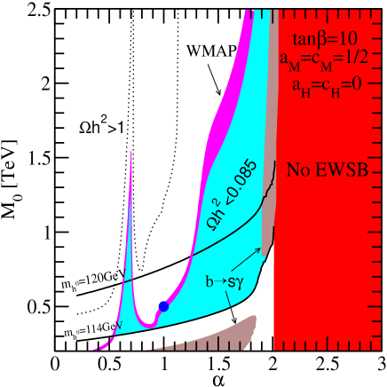
where cMsubscript𝑐𝑀c_{M} is a common parameter which parameterize the pattern of the pure modulus mediated masses for squarks and sleptons and cHsubscript𝑐𝐻c_{H} for soft Higgses. This choice of model parameters is denoted as a blue dot on the (α,M0)𝛼subscript𝑀0(\alpha,M_{0}) plane of Fig.1, which was taken from the figure 12 (c) in ref.[6]. In the Fig.1, the magenta stripe corresponds to the parameter region giving a thermal relic density consistent with the recent WMAP observation [11], i.e.formulae-sequence𝑖𝑒i.e. 0.085<ΩDMh2<0.1190.085subscriptΩ𝐷𝑀superscript20.1190.085<\Omega_{DM}h^{2}<0.119. The benchmark point is also consistent with constraints on particle spectra and bsγ𝑏𝑠𝛾b\rightarrow s\gamma branching ratio.


Refer to caption
Figure 1: Parameter space (α,M0)𝛼subscript𝑀0(\alpha,M_{0}) with aH=cH=0subscript𝑎𝐻subscript𝑐𝐻0a_{H}=c_{H}=0, aM=cM=1/2subscript𝑎𝑀subscript𝑐𝑀12a_{M}=c_{M}=1/2 and tanβ=10tan𝛽10{\rm tan\beta}=10. The blue point corresponds to our benchmark point, which satisfy relic density bound of WMAP observation and is consistent with other experimental constraints on particle masses and bsγ𝑏𝑠𝛾b\rightarrow s\gamma branching ratio.

The SUSY particle mass spectrum at the electroweak(EW) scale was computed by solving the RG equations with the model parameter set (10). For the gluino and the first two generation squark masses, we find

mg~=884.4GeV,md~L(u~L)=776.0(771.9)GeV,md~R(u~R)=733.5(741.8)GeV,formulae-sequencesubscript𝑚~𝑔884.4GeVformulae-sequencesubscript𝑚subscript~𝑑𝐿subscript~𝑢𝐿776.0771.9GeVsubscript𝑚subscript~𝑑𝑅subscript~𝑢𝑅733.5741.8GeV\displaystyle m_{\tilde{g}}=884.4~{}{\rm GeV},~{}m_{\tilde{d}_{L}(\tilde{u}_{L})}=776.0~{}(771.9)~{}{\rm GeV},~{}m_{\tilde{d}_{R}(\tilde{u}_{R})}=733.5~{}(741.8)~{}{\rm GeV}, (11)

while the masses of the third generation squarks are

mb~1(2)=703.9(734.6)GeV,mt~1(2)=545.3(782.0)GeVformulae-sequencesubscript𝑚subscript~𝑏12703.9734.6GeVsubscript𝑚subscript~𝑡12545.3782.0GeV\displaystyle m_{\tilde{b}_{1(2)}}=703.9~{}(734.6)~{}{\rm GeV},~{}m_{\tilde{t}_{1(2)}}=545.3~{}(782.0)~{}{\rm GeV} (12)

On the other hand, the slepton and sneutrino masses are

me~R(L)=382.0(431.5)GeV,mτ~1(2)=378.9(435.4)GeV,mν~L=424.1GeV.formulae-sequencesubscript𝑚subscript~𝑒𝑅𝐿382.0431.5GeVformulae-sequencesubscript𝑚subscript~𝜏12378.9435.4GeVsubscript𝑚subscript~𝜈𝐿424.1GeV\displaystyle m_{\tilde{e}_{R(L)}}=382.0~{}(431.5)~{}{\rm GeV},~{}m_{\tilde{\tau}_{1(2)}}=378.9~{}(435.4)~{}{\rm GeV},~{}m_{\tilde{\nu}_{L}}=424.1~{}{\rm GeV}. (13)

For the neutralino and chargino masses, we have

mχ~1,2,3,40={355.1,416.1,478.7,535.6}GeV,mχ~1,2±={408.2,533.5}GeV,formulae-sequencesubscript𝑚subscriptsuperscript~𝜒01234355.1416.1478.7535.6GeVsubscript𝑚subscriptsuperscript~𝜒plus-or-minus12408.2533.5GeV\displaystyle m_{\tilde{\chi}^{0}_{1,2,3,4}}=\{355.1,~{}416.1,~{}478.7,~{}535.6\}~{}{\rm GeV},~{}m_{\tilde{\chi}^{\pm}_{1,2}}=\{408.2,~{}533.5\}~{}{\rm GeV}, (14)

which correspond to the following bino,wino and Higgsino masses at electroweak scale,

M1=367GeV,M2=461GeV,μ=475GeV(fortanβ=10).formulae-sequencesubscript𝑀1367GeVformulae-sequencesubscript𝑀2461GeV𝜇475GeVfortan𝛽10\displaystyle M_{1}=367~{}{\rm GeV},~{}M_{2}=461~{}{\rm GeV},~{}\mu=475~{}{\rm GeV}~{}~{}({\rm for~{}tan\beta=10}). (15)

Finally, Higgs masses are given by

mh=115GeV,mH=528.6GeV,mA=528.3GeV,mH±=534.4GeV.formulae-sequencesubscript𝑚115GeVformulae-sequencesubscript𝑚𝐻528.6GeVformulae-sequencesubscript𝑚𝐴528.3GeVsubscript𝑚superscript𝐻plus-or-minus534.4GeV\displaystyle m_{h}=115~{}{\rm GeV},m_{H}=528.6~{}{\rm GeV},m_{A}=528.3~{}{\rm GeV},m_{H^{\pm}}=534.4~{}{\rm GeV}. (16)
Refer to caption
Refer to caption
Figure 2: The mass spectrum for (a) the benchmark point in mirage mediation and (b) a mSUGRA point. Both cases give the same mass for the lightest neutralino.

Fig. 2(a) shows the mass spectrum for the benchmark point. For comparison, we also show the spectrum of a mSUGRA point, which gives the same mass of neutralino LSP as the benchmark point, in Fig.2(b). One can notice that the spectrum of the benchmark point is quite degenerated, compared to the mSUGRA point.

With these mass parameters for the benchmark point, the neutralino LSP turns out to be bino-like, but𝑏𝑢𝑡but with non-negligible wino and Higgsino components. Neutralino pair annihilation into a gauge boson pair (ZZorW+W)𝑍𝑍orsuperscript𝑊superscript𝑊(ZZ~{}{\rm or}~{}W^{+}W^{-}) is then efficient so that thermal relic density of the neutralino LSP satisfies WMAP bound though the LSP is rather heavy (mχ~10355similar-tosubscript𝑚subscriptsuperscript~𝜒01355m_{\tilde{\chi}^{0}_{1}}\sim 355 GeV).

For the benchmark point, the ratio of gaugino masses at EW scale is given by M1:M2:M3=367:461:8501:1.26:2.32:subscript𝑀1subscript𝑀2:subscript𝑀3367:461:similar-to-or-equals8501:1.26:2.32M_{1}:M_{2}:M_{3}=367:461:850\simeq 1:1.26:2.32, which is quite degenerated comparing to the typical ratio M1:M2:M31:2:6:subscript𝑀1subscript𝑀2:similar-to-or-equalssubscript𝑀31:2:6M_{1}:M_{2}:M_{3}\simeq 1:2:6 for mSUGRA-like scenarios in which gaugino masses are unified at the GUT scale. For the benchmark point, the mass ratio of the gluino to the lightest neutralino is given by mg~/mχ~102.5similar-to-or-equalssubscript𝑚~𝑔subscript𝑚superscriptsubscript~𝜒102.5m_{\tilde{g}}/m_{\tilde{\chi}_{1}^{0}}\simeq 2.5, which is different from the typical mSUGRA predictions mg~/mχ~106greater-than-or-equivalent-tosubscript𝑚~𝑔subscript𝑚superscriptsubscript~𝜒106m_{\tilde{g}}/m_{\tilde{\chi}_{1}^{0}}\gtrsim 6 and therefore implies that the gaugino masses are NOT unified at the GUT scale. In the next subsection, we will see the mass ratio mg~/mχ~10subscript𝑚~𝑔subscript𝑚superscriptsubscript~𝜒10m_{\tilde{g}}/m_{\tilde{\chi}_{1}^{0}} can be measured experimentally so that we can get some information on SUSY breaking sector.

3.2 Monte Carlo Events

A Monte Carlo event sample of the SUSY signals for proton-proton collision at an energy of 14 TeV has been generated by PYTHIA 6.4 [12]. The event sample corresponds to 30 fb1𝑓superscript𝑏1fb^{-1} of integrated luminosity, which is expected with the 3 year running of the LHC at low luminosity. We have also generated SM background events i.e.,formulae-sequence𝑖𝑒i.e., tt¯𝑡¯𝑡t\bar{t} events equivalent to 30 fb1𝑓superscript𝑏1fb^{-1} of integrated luminosity and also W/Z+jet𝑊𝑍𝑗𝑒𝑡W/Z+jet, WW/WZ/ZZ𝑊𝑊𝑊𝑍𝑍𝑍WW/WZ/ZZ and QCD events, with less equivalent luminosity, in five logarithmic pTsubscript𝑝𝑇p_{T} bins for 50 GeV <pT<absentsubscript𝑝𝑇absent<p_{T}< 4000 GeV. The generated events have been further processed with a modified version of the fast detector simulation program PGS (Pretty Good Simulation)[13], which approximate an ATLAS- or CMS-like detector with reasonable efficiencies and fake rates.

The total production cross section for SUSY events at the LHC is similar-to\sim6.1 pb for the benchmark point, corresponding to 1.8×10⁵similar-toabsent1.8superscript105\sim 1.8\times 10^{5} events with 30 fb1𝑓superscript𝑏1fb^{-1} luminosity. Squarks and gluinos are expected to be copiously produced at the LHC, if mq~subscript𝑚~𝑞m_{\tilde{q}}, mg~1less-than-or-similar-tosubscript𝑚~𝑔1m_{\tilde{g}}\lesssim 1 TeV. With the masses of gluino and squarks in the Eq. (11), the production cross sections for the g~g~~𝑔~𝑔\tilde{g}\tilde{g}, g~q~~𝑔~𝑞\tilde{g}\tilde{q}, and q~q~~𝑞~𝑞\tilde{q}\tilde{q} pairs are about 0.30.30.3 pb, 2.72.72.7 pb and 2.02.02.0 pb, respectively, such that the gluino-squark pair production and the squark pair production dominate.

The produced squarks and gluinos decay generally in multistep. In the recent past, the following cascade decay chain of squark has been exploited in detail [9, 10];

q~Lχ~20ql~R±lqχ~10l+lq,subscript~𝑞𝐿subscriptsuperscript~𝜒02𝑞subscriptsuperscript~𝑙plus-or-minus𝑅superscript𝑙minus-or-plus𝑞subscriptsuperscript~𝜒01superscript𝑙superscript𝑙𝑞\displaystyle\tilde{q}_{L}\rightarrow\tilde{\chi}^{0}_{2}q\rightarrow\tilde{l}^{\pm}_{R}~{}l^{\mp}q\rightarrow\tilde{\chi}^{0}_{1}l^{+}l^{-}q, (17)

especially in mSUGRA framework. It was shown that it would be possible to reconstruct both upper edges for the l+lsuperscript𝑙superscript𝑙l^{+}l^{-}, l+lqsuperscript𝑙superscript𝑙𝑞l^{+}l^{-}q, and l±qsuperscript𝑙plus-or-minus𝑞l^{\pm}q mass distribution and a lower edge for the l+lqsuperscript𝑙superscript𝑙𝑞l^{+}l^{-}q mass coming from backwards decays of the χ~20subscriptsuperscript~𝜒02\tilde{\chi}^{0}_{2} in the q~Lsubscript~𝑞𝐿\tilde{q}_{L} rest frame. Those edge values of the mass distributions are given by the following analytic formulae, in terms of the particle masses involved in the decay chain;

Mllmax=[(mχ~202ml~R2)(ml~R2mχ~102)ml~R2]1/2,superscriptsubscript𝑀𝑙𝑙𝑚𝑎𝑥superscriptdelimited-[]superscriptsubscript𝑚superscriptsubscript~𝜒202superscriptsubscript𝑚subscript~𝑙𝑅2superscriptsubscript𝑚subscript~𝑙𝑅2superscriptsubscript𝑚superscriptsubscript~𝜒102superscriptsubscript𝑚subscript~𝑙𝑅212\displaystyle M_{ll}^{max}=\left[\frac{(m_{\tilde{\chi}_{2}^{0}}^{2}-m_{\tilde{l}_{R}}^{2})(m_{\tilde{l}_{R}}^{2}-m_{\tilde{\chi}_{1}^{0}}^{2})}{m_{\tilde{l}_{R}}^{2}}\right]^{1/2}, (18)
Mllqmax=[(mq~L2mχ~202)(mχ~202mχ~102)mχ~202]1/2,superscriptsubscript𝑀𝑙𝑙𝑞𝑚𝑎𝑥superscriptdelimited-[]superscriptsubscript𝑚subscript~𝑞𝐿2superscriptsubscript𝑚superscriptsubscript~𝜒202superscriptsubscript𝑚superscriptsubscript~𝜒202superscriptsubscript𝑚superscriptsubscript~𝜒102superscriptsubscript𝑚superscriptsubscript~𝜒20212\displaystyle M_{llq}^{max}=\left[\frac{(m_{\tilde{q}_{L}}^{2}-m_{\tilde{\chi}_{2}^{0}}^{2})(m_{\tilde{\chi}_{2}^{0}}^{2}-m_{\tilde{\chi}_{1}^{0}}^{2})}{m_{\tilde{\chi}_{2}^{0}}^{2}}\right]^{1/2}, (19)
Mlqmax(high)=[(mq~L2mχ~202)(mχ~202ml~R2)mχ~202]1/2,superscriptsubscript𝑀𝑙𝑞𝑚𝑎𝑥𝑖𝑔superscriptdelimited-[]superscriptsubscript𝑚subscript~𝑞𝐿2superscriptsubscript𝑚superscriptsubscript~𝜒202superscriptsubscript𝑚superscriptsubscript~𝜒202superscriptsubscript𝑚subscript~𝑙𝑅2superscriptsubscript𝑚superscriptsubscript~𝜒20212\displaystyle M_{lq}^{max}(high)=\left[\frac{(m_{\tilde{q}_{L}}^{2}-m_{\tilde{\chi}_{2}^{0}}^{2})(m_{\tilde{\chi}_{2}^{0}}^{2}-m_{\tilde{l}_{R}}^{2})}{m_{\tilde{\chi}_{2}^{0}}^{2}}\right]^{1/2}, (20)
(Mllqmin)2superscriptsuperscriptsubscript𝑀𝑙𝑙𝑞𝑚𝑖𝑛2\displaystyle(M_{llq}^{min})^{2} =\displaystyle= 14mχ~202ml~R2[mχ~102mχ~204+3mχ~102mχ~202ml~R2mχ~204ml~R2mχ~202ml~R4\displaystyle\frac{1}{4m_{\tilde{\chi}_{2}^{0}}^{2}m_{\tilde{l}_{R}}^{2}}\big{[}-m_{\tilde{\chi}_{1}^{0}}^{2}m_{\tilde{\chi}_{2}^{0}}^{4}+3m_{\tilde{\chi}_{1}^{0}}^{2}m_{\tilde{\chi}_{2}^{0}}^{2}m_{\tilde{l}_{R}}^{2}-m_{\tilde{\chi}_{2}^{0}}^{4}m_{\tilde{l}_{R}}^{2}-m_{\tilde{\chi}_{2}^{0}}^{2}m_{\tilde{l}_{R}}^{4}
\displaystyle- mχ~102mχ~202mq~L2mχ~102ml~R2mq~L2+3mχ~202ml~R2mq~L2ml~R4mq~L2superscriptsubscript𝑚superscriptsubscript~𝜒102superscriptsubscript𝑚superscriptsubscript~𝜒202superscriptsubscript𝑚subscript~𝑞𝐿2superscriptsubscript𝑚superscriptsubscript~𝜒102superscriptsubscript𝑚subscript~𝑙𝑅2superscriptsubscript𝑚subscript~𝑞𝐿23superscriptsubscript𝑚superscriptsubscript~𝜒202superscriptsubscript𝑚subscript~𝑙𝑅2superscriptsubscript𝑚subscript~𝑞𝐿2superscriptsubscript𝑚subscript~𝑙𝑅4superscriptsubscript𝑚subscript~𝑞𝐿2\displaystyle m_{\tilde{\chi}_{1}^{0}}^{2}m_{\tilde{\chi}_{2}^{0}}^{2}m_{\tilde{q}_{L}}^{2}-m_{\tilde{\chi}_{1}^{0}}^{2}m_{\tilde{l}_{R}}^{2}m_{\tilde{q}_{L}}^{2}+3m_{\tilde{\chi}_{2}^{0}}^{2}m_{\tilde{l}_{R}}^{2}m_{\tilde{q}_{L}}^{2}-m_{\tilde{l}_{R}}^{4}m_{\tilde{q}_{L}}^{2}
+\displaystyle+ (mχ~202mq~L2)(mχ~104+ml~R4)(mχ~202+ml~R2)2+2mχ~102ml~R2(mχ~2046mχ~202ml~R2+ml~R4)].\displaystyle(m_{\tilde{\chi}_{2}^{0}}^{2}-m_{\tilde{q}_{L}}^{2})\sqrt{(m_{\tilde{\chi}_{1}^{0}}^{4}+m_{\tilde{l}_{R}}^{4})(m_{\tilde{\chi}_{2}^{0}}^{2}+m_{\tilde{l}_{R}}^{2})^{2}+2m_{\tilde{\chi}_{1}^{0}}^{2}m_{\tilde{l}_{R}}^{2}(m_{\tilde{\chi}_{2}^{0}}^{4}-6m_{\tilde{\chi}_{2}^{0}}^{2}m_{\tilde{l}_{R}}^{2}+m_{\tilde{l}_{R}}^{4})}~{}\big{]}.

We can also measure the upper edge of the distribution of the smaller𝑠𝑚𝑎𝑙𝑙𝑒𝑟smaller of the two possible lq𝑙𝑞lq masses formed by combining two leptons with a quark jet [14];

Mlqmax(low)superscriptsubscript𝑀𝑙𝑞𝑚𝑎𝑥𝑙𝑜𝑤\displaystyle M_{lq}^{max}(low) =\displaystyle= [(mq~L2mχ~202)(me~R2mχ~102)2me~R2mχ~102]1/2for2me~R2(mχ~102+mχ~202)<0.superscriptdelimited-[]superscriptsubscript𝑚subscript~𝑞𝐿2superscriptsubscript𝑚superscriptsubscript~𝜒202superscriptsubscript𝑚subscript~𝑒𝑅2superscriptsubscript𝑚superscriptsubscript~𝜒1022superscriptsubscript𝑚subscript~𝑒𝑅2superscriptsubscript𝑚superscriptsubscript~𝜒10212for2superscriptsubscript𝑚subscript~𝑒𝑅2superscriptsubscript𝑚superscriptsubscript~𝜒102superscriptsubscript𝑚superscriptsubscript~𝜒2020\displaystyle\left[\frac{(m_{\tilde{q}_{L}}^{2}-m_{\tilde{\chi}_{2}^{0}}^{2})(m_{\tilde{e}_{R}}^{2}-m_{\tilde{\chi}_{1}^{0}}^{2})}{2m_{\tilde{e}_{R}}^{2}-m_{\tilde{\chi}_{1}^{0}}^{2}}\right]^{1/2}~{}{\rm for}~{}2m_{\tilde{e}_{R}}^{2}-(m_{\tilde{\chi}_{1}^{0}}^{2}+m_{\tilde{\chi}_{2}^{0}}^{2})<0. (22)
=\displaystyle= [(mq~L2mχ~202)(mχ~202me~R2)mχ~202]1/2for2me~R2(mχ~102+mχ~202)>0.superscriptdelimited-[]superscriptsubscript𝑚subscript~𝑞𝐿2superscriptsubscript𝑚superscriptsubscript~𝜒202superscriptsubscript𝑚superscriptsubscript~𝜒202superscriptsubscript𝑚subscript~𝑒𝑅2superscriptsubscript𝑚superscriptsubscript~𝜒20212for2superscriptsubscript𝑚subscript~𝑒𝑅2superscriptsubscript𝑚superscriptsubscript~𝜒102superscriptsubscript𝑚superscriptsubscript~𝜒2020\displaystyle\left[\frac{(m_{\tilde{q}_{L}}^{2}-m_{\tilde{\chi}_{2}^{0}}^{2})(m_{\tilde{\chi}_{2}^{0}}^{2}-m_{\tilde{e}_{R}}^{2})}{m_{\tilde{\chi}_{2}^{0}}^{2}}\right]^{1/2}~{}{\rm for}~{}2m_{\tilde{e}_{R}}^{2}-(m_{\tilde{\chi}_{1}^{0}}^{2}+m_{\tilde{\chi}_{2}^{0}}^{2})>0.

From the kinematic edge measurements, the SUSY particle masses might be then determined without relying on a model. For the benchmark point, we can notice that mχ~20>me~Rsubscript𝑚subscriptsuperscript~𝜒02subscript𝑚subscript~𝑒𝑅m_{\tilde{\chi}^{0}_{2}}>m_{\tilde{e}_{R}}. Therefore, the cascade decay chain (17) is indeed open so that the well-established method of the kinematic edge measurements can be applied to our case.

In order to reduce the SM background to a negligible level, we apply the following event selection cuts;

(1) At least three jets with PT1>200subscript𝑃𝑇1200P_{T1}>200 GeV and PT2,3>50subscript𝑃𝑇2350P_{T2,3}>50 GeV.

(2) Missing transverse energy, ETmiss>200GeV.superscriptsubscript𝐸𝑇𝑚𝑖𝑠𝑠200GeVE_{T}^{miss}>200~{}{\rm GeV}.

(3) ETmiss/Meff>0.2superscriptsubscript𝐸𝑇𝑚𝑖𝑠𝑠subscript𝑀𝑒𝑓𝑓0.2E_{T}^{miss}/M_{eff}>0.2, where MeffPT1+PT2+PT3+PT4+ETmiss+leptonsPTlsubscript𝑀𝑒𝑓𝑓subscript𝑃𝑇1subscript𝑃𝑇2subscript𝑃𝑇3subscript𝑃𝑇4superscriptsubscript𝐸𝑇𝑚𝑖𝑠𝑠subscript𝑙𝑒𝑝𝑡𝑜𝑛𝑠subscript𝑃𝑇𝑙M_{eff}\equiv P_{T1}+P_{T2}+P_{T3}+P_{T4}+E_{T}^{miss}+\sum_{leptons}P_{Tl}

(4) At least two isolated leptons of opposite charge, with PT>10subscript𝑃𝑇10P_{T}>10 GeV and |η|<2.5𝜂2.5|\eta|<2.5.

(5) Transverse sphericity ST>0.1subscript𝑆𝑇0.1S_{T}>0.1.

(6) No b-jets.


Refer to caption
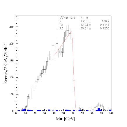
Figure 3: Dilepton (e+e+μ+μe±μsuperscript𝑒superscript𝑒superscript𝜇superscript𝜇superscript𝑒plus-or-minussuperscript𝜇minus-or-pluse^{+}e^{-}+\mu^{+}\mu^{-}-e^{\pm}\mu^{\mp}) invariant mass distributions for the benchmark point. Blue histogram corresponds to SM background.

Following the analysis in Ref.[9], we have then calculated various invariant mass distributions for the benchmark point. The dilepton invariant mass distribution is shown in the Fig. 3. Here, the e+e+μ+μe±μsuperscript𝑒superscript𝑒superscript𝜇superscript𝜇superscript𝑒plus-or-minussuperscript𝜇minus-or-pluse^{+}e^{-}+\mu^{+}\mu^{-}-e^{\pm}\mu^{\mp} combination was used in order to cancel contributions for two independent decays and reduce combinatorial background. The SM backgrounds which denoted as blue histogram on the plot, are negligible with the above event selection cuts, as expected from previous studies [7, 9]. We find a clear end point in the dilepton mass distribution. A Gaussian-smeared triangular fit to the distribution gives Mllmax=60.61±0.13superscriptsubscript𝑀𝑙𝑙𝑚𝑎𝑥plus-or-minus60.610.13M_{ll}^{max}=60.61\pm 0.13 GeV, which is 0.3%similar-toabsentpercent0.3\sim 0.3\% lower than the calculated value of Mllmax=60.8superscriptsubscript𝑀𝑙𝑙𝑚𝑎𝑥60.8M_{ll}^{max}=60.8 GeV for the decays χ~20l~Rl±χ~10l+lsuperscriptsubscript~𝜒20subscript~𝑙𝑅superscript𝑙plus-or-minussuperscriptsubscript~𝜒10superscript𝑙superscript𝑙\tilde{\chi}_{2}^{0}\rightarrow\tilde{l}_{R}l^{\pm}\rightarrow\tilde{\chi}_{1}^{0}l^{+}l^{-}.

Refer to caption
Refer to caption
Refer to caption
Refer to caption
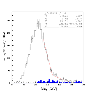
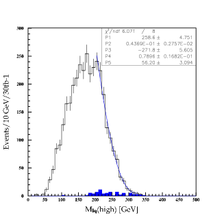
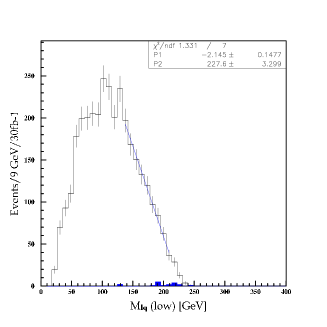
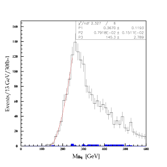
Figure 4: Distributions for (a) the smaller of the two Mllqsubscript𝑀𝑙𝑙𝑞M_{llq}, (b) the larger of two Mlqsubscript𝑀𝑙𝑞M_{lq}, (c) the smaller of the two Mlqsubscript𝑀𝑙𝑞M_{lq}, and (d) the larger of the two Mllqsubscript𝑀𝑙𝑙𝑞M_{llq} with Mll>Mllmax/2subscript𝑀𝑙𝑙superscriptsubscript𝑀𝑙𝑙𝑚𝑎𝑥2M_{ll}>M_{ll}^{max}/\sqrt{2}.

The dilepton plus jet invariant mass Mllqsubscript𝑀𝑙𝑙𝑞M_{llq} has been also calculated by combining the dilepton with one of the two hardest PTsubscript𝑃𝑇P_{T} jets. The two hardest jets are expected to come from squark decays q~χ~q~𝑞~𝜒𝑞\tilde{q}\rightarrow\tilde{\chi}q as dominant production processes result in a pair of squark . The distribution for the smaller of the two possible llq𝑙𝑙𝑞llq masses is shown in Fig. 4(a). The upper edge value of the l+lqsuperscript𝑙superscript𝑙𝑞l^{+}l^{-}q masses is given by Mllqmax=341.5±3.6superscriptsubscript𝑀𝑙𝑙𝑞𝑚𝑎𝑥plus-or-minus341.53.6M_{llq}^{max}=341.5\pm 3.6 GeV, which is obtained from a Gaussian smeared fit plus a linear background. The fitted value is consistent with the calculated value of Mllqmax=341.4superscriptsubscript𝑀𝑙𝑙𝑞𝑚𝑎𝑥341.4M_{llq}^{max}=341.4 GeV for the decays q~Lχ~20ql~R±lqχ~10l+lqsubscript~𝑞𝐿superscriptsubscript~𝜒20𝑞superscriptsubscript~𝑙𝑅plus-or-minussuperscript𝑙minus-or-plus𝑞superscriptsubscript~𝜒10superscript𝑙superscript𝑙𝑞\tilde{q}_{L}\rightarrow\tilde{\chi}_{2}^{0}q\rightarrow\tilde{l}_{R}^{\pm}l^{\mp}q\rightarrow\tilde{\chi}_{1}^{0}l^{+}l^{-}q (with mq~L=776subscript𝑚subscript~𝑞𝐿776m_{\tilde{q}_{L}}=776 GeV).

Now, we further require that one Mllqsubscript𝑀𝑙𝑙𝑞M_{llq} should be less than 350 GeV and the other greater. Two l±qsuperscript𝑙plus-or-minus𝑞l^{\pm}q masses are then calculated using the combination of l+lqsuperscript𝑙superscript𝑙𝑞l^{+}l^{-}q with the smaller Mllq(<350GeV)annotatedsubscript𝑀𝑙𝑙𝑞absent350GeVM_{llq}~{}(<350~{}{\rm GeV}). Fig. 4(b) shows the mass distribution of the larger𝑙𝑎𝑟𝑔𝑒𝑟larger of the two l±qsuperscript𝑙plus-or-minus𝑞l^{\pm}q system. A fit to the mass distribution near the end point is also shown, which yield an upper edge value Mlqmax(high)=258.6±4.8superscriptsubscript𝑀𝑙𝑞𝑚𝑎𝑥𝑖𝑔plus-or-minus258.64.8M_{lq}^{max}(high)=258.6\pm 4.8 GeV, which is consistent with the calculated value of Mlqmax(high)=259.7superscriptsubscript𝑀𝑙𝑞𝑚𝑎𝑥𝑖𝑔259.7M_{lq}^{max}(high)=259.7 GeV.

The mass distribution of the smaller𝑠𝑚𝑎𝑙𝑙𝑒𝑟smaller of the two Mlqsubscript𝑀𝑙𝑞M_{lq} is shown in Fig. 4(c). The upper edge value of the distribution from a linear fit is given by Mlqmax(low)=227.6±3.3superscriptsubscript𝑀𝑙𝑞𝑚𝑎𝑥𝑙𝑜𝑤plus-or-minus227.63.3M_{lq}^{max}(low)=227.6\pm 3.3 GeV, which is consistent with the calculated value of Mlqmax(low)=226.5superscriptsubscript𝑀𝑙𝑞𝑚𝑎𝑥𝑙𝑜𝑤226.5M_{lq}^{max}(low)=226.5 GeV.

The lower edge for l+lqsuperscript𝑙superscript𝑙𝑞l^{+}l^{-}q mass can be reconstructed from the larger of the two possible l+lqsuperscript𝑙superscript𝑙𝑞l^{+}l^{-}q masses, with additional requirement Mllmax/2<Mll<Mllmaxsuperscriptsubscript𝑀𝑙𝑙𝑚𝑎𝑥2subscript𝑀𝑙𝑙superscriptsubscript𝑀𝑙𝑙𝑚𝑎𝑥M_{ll}^{max}/\sqrt{2}<M_{ll}<M_{ll}^{max}. The resulting distribution is shown in Fig. 4(d). A fit to the distribution gives Mllqmin=145.3±2.8superscriptsubscript𝑀𝑙𝑙𝑞𝑚𝑖𝑛plus-or-minus145.32.8M_{llq}^{min}=145.3\pm 2.8 GeV, which is consistent with the generated value Mllqmin=145.4superscriptsubscript𝑀𝑙𝑙𝑞𝑚𝑖𝑛145.4M_{llq}^{min}=145.4 GeV.

From the above five edge measurements for the q~Lsubscript~𝑞𝐿\tilde{q}_{L} cascade decays (17), we can determine the masses of q~Lsubscript~𝑞𝐿\tilde{q}_{L}, l~Rsubscript~𝑙𝑅\tilde{l}_{R}, χ~20superscriptsubscript~𝜒20\tilde{\chi}_{2}^{0} and χ~10superscriptsubscript~𝜒10\tilde{\chi}_{1}^{0} using the eqs. (18-22).

Refer to caption
Refer to caption
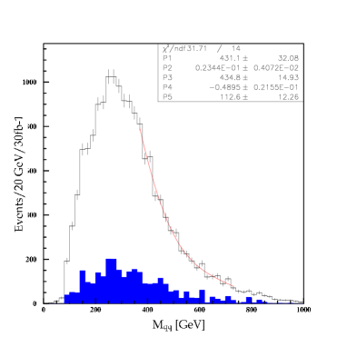
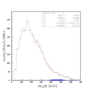
Figure 5: Dijet invariant mass distribution (a) without dilepton and (b) with dilepton.

With given masses of χ~10superscriptsubscript~𝜒10\tilde{\chi}_{1}^{0} and χ~20superscriptsubscript~𝜒20\tilde{\chi}_{2}^{0}, we can get information for gluino and squark masses from the following gluino decay into right-handed squark plus quark;

g~q~Rqχ~10qq.~𝑔subscript~𝑞𝑅𝑞superscriptsubscript~𝜒10𝑞𝑞\displaystyle\tilde{g}\rightarrow\tilde{q}_{R}q\rightarrow\tilde{\chi}_{1}^{0}qq. (23)

The maximal value of the two jet invariant mass for the gluino decays (23) is given by

Mqqmax=[(mg~2mq~R2)(mq~R2mχ~102)mq~R2]1/2.superscriptsubscript𝑀𝑞𝑞𝑚𝑎𝑥superscriptdelimited-[]superscriptsubscript𝑚~𝑔2superscriptsubscript𝑚subscript~𝑞𝑅2superscriptsubscript𝑚subscript~𝑞𝑅2superscriptsubscript𝑚superscriptsubscript~𝜒102superscriptsubscript𝑚subscript~𝑞𝑅212\displaystyle M_{qq}^{max}=\left[\frac{(m_{\tilde{g}}^{2}-m_{\tilde{q}_{R}}^{2})(m_{\tilde{q}_{R}}^{2}-m_{\tilde{\chi}_{1}^{0}}^{2})}{m_{\tilde{q}_{R}}^{2}}\right]^{1/2}. (24)

At the LHC, gluino would be produced mainly from g~q~~𝑔~𝑞\tilde{g}\tilde{q} or g~g~~𝑔~𝑔\tilde{g}\tilde{g} pair production. In order to obtain event sample for the gluino decay (23), the following event selection cuts are imposed;

(1) At least 3 jets with PT1>200subscript𝑃𝑇1200P_{T1}>200 GeV, PT2>150subscript𝑃𝑇2150P_{T2}>150 GeV and PT3>100subscript𝑃𝑇3100P_{T3}>100 GeV.

(2) ETmiss>350superscriptsubscript𝐸𝑇𝑚𝑖𝑠𝑠350E_{T}^{miss}>350 GeV and ETmiss/Meff>0.25superscriptsubscript𝐸𝑇𝑚𝑖𝑠𝑠subscript𝑀𝑒𝑓𝑓0.25E_{T}^{miss}/M_{eff}>0.25.

(3) Transverse sphericity ST>0.15subscript𝑆𝑇0.15S_{T}>0.15.

(4) No b-jets and No leptons.

In the selection cuts, we required rather hard PT3>100subscript𝑃𝑇3100P_{T3}>100 GeV in order to reduce q~q~~𝑞~𝑞{\tilde{q}}{\tilde{q}} production events. After the selection cuts, we calculate dijet invariant mass Mqqsubscript𝑀𝑞𝑞M_{qq} using the three hardest jets. The smallest Mqqsubscript𝑀𝑞𝑞M_{qq} among the three possible combinations is then shown in Fig. 5 (a). The Mqqsubscript𝑀𝑞𝑞M_{qq} distribution is fitted near end point by a Gaussian smeared linear function with a linear background. The resulting edge value is given by Mqqmax=431.1±32.1superscriptsubscript𝑀𝑞𝑞𝑚𝑎𝑥plus-or-minus431.132.1M_{qq}^{max}=431.1\pm 32.1 GeV, which is consistent with the calculated one Mqqmax=432.4superscriptsubscript𝑀𝑞𝑞𝑚𝑎𝑥432.4M_{qq}^{max}=432.4 GeV (with mq~R=733.5subscript𝑚subscript~𝑞𝑅733.5m_{\tilde{q}_{R}}=733.5 GeV).

Additional information on mg~subscript𝑚~𝑔m_{\tilde{g}} and mq~Rsubscript𝑚subscript~𝑞𝑅m_{\tilde{q}_{R}} might be provided by the following cascade decay of gluino,

g~q~Rqχ~20qq(χ~10llqq),~𝑔subscript~𝑞𝑅𝑞annotatedsuperscriptsubscript~𝜒20𝑞𝑞absentsuperscriptsubscript~𝜒10𝑙𝑙𝑞𝑞\displaystyle\tilde{g}\rightarrow\tilde{q}_{R}q\rightarrow\tilde{\chi}_{2}^{0}qq~{}(\rightarrow\tilde{\chi}_{1}^{0}llqq), (25)

for which the upper edge value of the two jet invariant mass distribution is given by

Mqqmax(ll)=[(mg~2mq~R2)(mq~R2mχ~202)mq~R2]1/2.superscriptsubscript𝑀𝑞𝑞𝑚𝑎𝑥𝑙𝑙superscriptdelimited-[]superscriptsubscript𝑚~𝑔2superscriptsubscript𝑚subscript~𝑞𝑅2superscriptsubscript𝑚subscript~𝑞𝑅2superscriptsubscript𝑚superscriptsubscript~𝜒202superscriptsubscript𝑚subscript~𝑞𝑅212\displaystyle M_{qq}^{max}(ll)=\left[\frac{(m_{\tilde{g}}^{2}-m_{\tilde{q}_{R}}^{2})(m_{\tilde{q}_{R}}^{2}-m_{\tilde{\chi}_{2}^{0}}^{2})}{m_{\tilde{q}_{R}}^{2}}\right]^{1/2}. (26)

In the gluino cascade decay (25), we consider the right-handed squark decay into χ~20superscriptsubscript~𝜒20\tilde{\chi}_{2}^{0} rather than χ~10superscriptsubscript~𝜒10\tilde{\chi}_{1}^{0}, where the χ~20superscriptsubscript~𝜒20\tilde{\chi}_{2}^{0} further undergoes the dileptonic decay. In the benchmark point, branching ratio BR(q~Rχ~20q)=11%𝐵𝑅subscript~𝑞𝑅superscriptsubscript~𝜒20𝑞percent11BR(\tilde{q}_{R}\rightarrow\tilde{\chi}_{2}^{0}q)=11\% is comparable to BR(q~Lχ~20q)=18.5%𝐵𝑅subscript~𝑞𝐿superscriptsubscript~𝜒20𝑞percent18.5BR(\tilde{q}_{L}\rightarrow\tilde{\chi}_{2}^{0}q)=18.5\%. This is because the gaugino masses are quite degenerated (i.e.M2/M11.26)formulae-sequence𝑖𝑒similar-tosubscript𝑀2subscript𝑀11.26(i.e.~{}M_{2}/M_{1}\sim 1.26) at EW scale so that χ~20superscriptsubscript~𝜒20\tilde{\chi}_{2}^{0} has sizable bino-component in the benchmark point, which is in contrast to the typical mSUGRA case where χ~20superscriptsubscript~𝜒20\tilde{\chi}_{2}^{0} is almost wino-like and therefore BR(q~Rχ~20q)𝐵𝑅subscript~𝑞𝑅superscriptsubscript~𝜒20𝑞BR(\tilde{q}_{R}\rightarrow\tilde{\chi}_{2}^{0}q) is negligible. Furthermore, the gluino branching ratio of BR(g~q~Rq)19%similar-to-or-equals𝐵𝑅~𝑔subscript~𝑞𝑅𝑞percent19BR(\tilde{g}\rightarrow\tilde{q}_{R}q)\simeq 19\% is larger than BR(g~q~Lq)11.2%similar-to-or-equals𝐵𝑅~𝑔subscript~𝑞𝐿𝑞percent11.2BR(\tilde{g}\rightarrow\tilde{q}_{L}q)\simeq 11.2\% for q=u,d so that the decay chain of g~q~Rqχ~20qq~𝑔subscript~𝑞𝑅𝑞superscriptsubscript~𝜒20𝑞𝑞\tilde{g}\rightarrow\tilde{q}_{R}q\rightarrow\tilde{\chi}_{2}^{0}qq is comparable to that of g~q~Lqχ~20qq~𝑔subscript~𝑞𝐿𝑞superscriptsubscript~𝜒20𝑞𝑞\tilde{g}\rightarrow\tilde{q}_{L}q\rightarrow\tilde{\chi}_{2}^{0}qq. Considering the squark masses that mq~R<mq~Lsubscript𝑚subscript~𝑞𝑅subscript𝑚subscript~𝑞𝐿m_{\tilde{q}_{R}}<m_{\tilde{q}_{L}}, the upper edge value of two jet invariant mass for χ~20qqsuperscriptsubscript~𝜒20𝑞𝑞\tilde{\chi}_{2}^{0}qq events is essentially determined by the Eq. (26), which involves mq~Rsubscript𝑚subscript~𝑞𝑅m_{\tilde{q}_{R}} rather than mq~Lsubscript𝑚subscript~𝑞𝐿m_{\tilde{q}_{L}}.

In order to select events which include decay chain (25), we require

(1) At least 3 jets with PT1>100subscript𝑃𝑇1100P_{T1}>100 GeV and PT2,3>50subscript𝑃𝑇2350P_{T2,3}>50 GeV

(2) ETmiss>200superscriptsubscript𝐸𝑇𝑚𝑖𝑠𝑠200E_{T}^{miss}>200 GeV and Meff/ETmiss>0.2subscript𝑀𝑒𝑓𝑓superscriptsubscript𝐸𝑇𝑚𝑖𝑠𝑠0.2M_{eff}/E_{T}^{miss}>0.2

(3) At least two isolated leptons with opposite charge

(4) Mll<61subscript𝑀𝑙𝑙61M_{ll}<61 GeV and the smallest Mllq<350subscript𝑀𝑙𝑙𝑞350M_{llq}<350 GeV

(5) Transverse sphericity ST>0.1subscript𝑆𝑇0.1S_{T}>0.1

(6) No b-jets

After the selection cut, dijet invariant mass was calculated using the jet, which gives the smallest Mllqsubscript𝑀𝑙𝑙𝑞M_{llq}, with third and fourth (if any) energetic jets. The smaller of the two possible dijet mass is then shown in Fig. 5 (b). A fit to the distribution gives Mqqmax(ll)=405.7±8.6superscriptsubscript𝑀𝑞𝑞𝑚𝑎𝑥𝑙𝑙plus-or-minus405.78.6M_{qq}^{max}(ll)=405.7\pm 8.6 GeV, which is consistent with the calculated value of Mqqmax(ll)=406.9superscriptsubscript𝑀𝑞𝑞𝑚𝑎𝑥𝑙𝑙406.9M_{qq}^{max}(ll)=406.9 GeV (with mq~R=733.5subscript𝑚subscript~𝑞𝑅733.5m_{\tilde{q}_{R}}=733.5 GeV).

The upper edge measurements of two dijet invariant masses provide lower limits on the gluino and squark masses and a strong correlation between mg~subscript𝑚~𝑔m_{\tilde{g}} and mq~Rsubscript𝑚subscript~𝑞𝑅m_{\tilde{q}_{R}}, but without constraint on the upper limit on the masses.
Refer to caption
Refer to caption
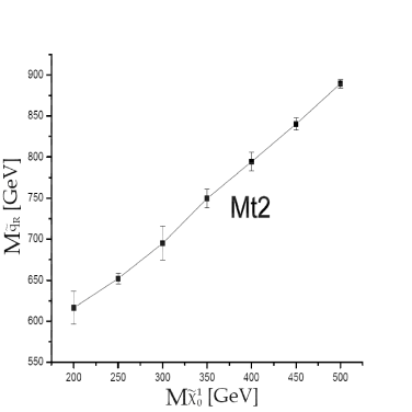
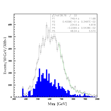
Figure 6: (a) The MT2subscript𝑀𝑇2M_{T2} distribution with the input value of mχ=350subscript𝑚𝜒350m_{\chi}=350 GeV as an example. (b) A relation between mq~Rsubscript𝑚subscript~𝑞𝑅m_{\tilde{q}_{R}} and mχ~10subscript𝑚superscriptsubscript~𝜒10m_{\tilde{\chi}_{1}^{0}} from the MT2subscript𝑀𝑇2M_{T2} analysis.

In order to further constrain the right-handed squark mass, we consider squark pair production and their subsequent decay into two quarks plus two LSPs;

q~1Rq~2Rq1χ~10q2χ~10,subscript~𝑞1𝑅subscript~𝑞2𝑅subscript𝑞1superscriptsubscript~𝜒10subscript𝑞2superscriptsubscript~𝜒10\displaystyle{\tilde{q}_{1R}}{\tilde{q}_{2R}}\rightarrow q_{1}{\tilde{\chi}}_{1}^{0}q_{2}{\tilde{\chi}}_{1}^{0}, (27)

and construct another variable MT2subscript𝑀𝑇2M_{T2} [15], which is defined by

MT22min𝐩T1χ+𝐩T2χ=𝐩Tmiss[max{mT2(𝐩Tq1,𝐩T1χ),mT2(𝐩Tq2,𝐩T2χ)}],superscriptsubscript𝑀𝑇22subscriptsuperscriptsubscript𝐩𝑇1𝜒superscriptsubscript𝐩𝑇2𝜒superscriptsubscript𝐩𝑇𝑚𝑖𝑠𝑠maxsuperscriptsubscript𝑚𝑇2superscriptsubscript𝐩𝑇subscript𝑞1superscriptsubscript𝐩𝑇1𝜒superscriptsubscript𝑚𝑇2superscriptsubscript𝐩𝑇subscript𝑞2superscriptsubscript𝐩𝑇2𝜒\displaystyle M_{T2}^{2}\equiv\min_{{\bf p}_{T1}^{\chi}+{\bf p}_{T2}^{\chi}={\bf p}_{T}^{miss}}\left[{\rm max}\{m_{T}^{2}({\rm{\bf p}}_{T}^{q_{1}},{\rm{\bf p}}_{T1}^{\chi}),m_{T}^{2}({\rm{\bf p}}_{T}^{q_{2}},{\rm{\bf p}}_{T2}^{\chi})\}\right], (28)

where

mT22(𝐩Tq,𝐤Tχ)mq2+mχ2+2(ETqETχ𝐩Tq𝐤Tχ),superscriptsubscript𝑚𝑇22superscriptsubscript𝐩𝑇𝑞superscriptsubscript𝐤𝑇𝜒superscriptsubscript𝑚𝑞2superscriptsubscript𝑚𝜒22superscriptsubscript𝐸𝑇𝑞superscriptsubscript𝐸𝑇𝜒superscriptsubscript𝐩𝑇𝑞superscriptsubscript𝐤𝑇𝜒\displaystyle m_{T2}^{2}({\bf p}_{T}^{q},{\bf k}_{T}^{\chi})\equiv m_{q}^{2}+m_{\chi}^{2}+2(E_{T}^{q}E_{T}^{\chi}-{\bf p}_{T}^{q}\cdot{\bf k}_{T}^{\chi}), (29)
ETq=|𝐩Tq|2+mq2,ETχ=|𝐤Tχ|2+mχ2.formulae-sequencesuperscriptsubscript𝐸𝑇𝑞superscriptsuperscriptsubscript𝐩𝑇𝑞2superscriptsubscript𝑚𝑞2superscriptsubscript𝐸𝑇𝜒superscriptsuperscriptsubscript𝐤𝑇𝜒2superscriptsubscript𝑚𝜒2\displaystyle E_{T}^{q}=\sqrt{|{\bf p}_{T}^{q}|^{2}+m_{q}^{2}},~{}~{}E_{T}^{\chi}=\sqrt{|{\bf k}_{T}^{\chi}|^{2}+m_{\chi}^{2}}. (30)

Here, 𝐩Tq1superscriptsubscript𝐩𝑇subscript𝑞1{\bf p}_{T}^{q_{1}} and 𝐩Tq2superscriptsubscript𝐩𝑇subscript𝑞2{\bf p}_{T}^{q_{2}} denote the transverse momentum of quark-jets from the squark decays and 𝐩Tmisssuperscriptsubscript𝐩𝑇𝑚𝑖𝑠𝑠{\bf p}_{T}^{miss} is the observed missing transverse momentum and mχsubscript𝑚𝜒m_{\chi} is an estimate of the lightest neutralino mass. The MT2subscript𝑀𝑇2M_{T2} distribution has an endpoint at the squark mass mq~Rsubscript𝑚subscript~𝑞𝑅m_{\tilde{q}_{R}} when the input mχsubscript𝑚𝜒m_{\chi} is equal to the correct mχ~10subscript𝑚superscriptsubscript~𝜒10m_{\tilde{\chi}_{1}^{0}} value. In general we obtain a relation between mq~Rsubscript𝑚subscript~𝑞𝑅m_{\tilde{q}_{R}} and mχ~10subscript𝑚superscriptsubscript~𝜒10m_{\tilde{\chi}_{1}^{0}}.

In order to have event sample for the squark pair production and their subsequent decay (27), the following event selection cuts are required;

(1) At least two jets with PT1>300subscript𝑃𝑇1300P_{T1}>300 GeV, PT2>50subscript𝑃𝑇250P_{T2}>50 GeV

(2) ETmiss>200superscriptsubscript𝐸𝑇𝑚𝑖𝑠𝑠200E_{T}^{miss}>200 GeV, Meff/ETmiss>0.3subscript𝑀𝑒𝑓𝑓superscriptsubscript𝐸𝑇𝑚𝑖𝑠𝑠0.3M_{eff}/E_{T}^{miss}>0.3

(3) Transverse sphericity ST>0.15subscript𝑆𝑇0.15S_{T}>0.15

(4) No leptons, no b-jets.

Fig. 6(a) shows an example of MT2subscript𝑀𝑇2M_{T2} distribution with an input value of mχ=350subscript𝑚𝜒350m_{\chi}=350 GeV. From a fit to the distribution, we obtain mq~R=749±12subscript𝑚subscript~𝑞𝑅plus-or-minus74912m_{\tilde{q}_{R}}=749\pm 12 GeV for the example. A general relation between mq~Rsubscript𝑚subscript~𝑞𝑅m_{\tilde{q}_{R}} and mχ~10subscript𝑚superscriptsubscript~𝜒10m_{\tilde{\chi}_{1}^{0}} from the MT2subscript𝑀𝑇2M_{T2} analysis is shown in Fig. 6(b).

Refer to caption
Figure 7: Probability distribution of (a) mχ~10subscript𝑚superscriptsubscript~𝜒10m_{\tilde{\chi}_{1}^{0}}, (b) mχ~20mχ~10subscript𝑚superscriptsubscript~𝜒20subscript𝑚superscriptsubscript~𝜒10m_{\tilde{\chi}_{2}^{0}}-m_{\tilde{\chi}_{1}^{0}}, (c) ml~Rmχ~10subscript𝑚subscript~𝑙𝑅subscript𝑚superscriptsubscript~𝜒10m_{\tilde{l}_{R}}-m_{\tilde{\chi}_{1}^{0}}, (d) mq~Lmχ~10subscript𝑚subscript~𝑞𝐿subscript𝑚superscriptsubscript~𝜒10m_{\tilde{q}_{L}}-m_{\tilde{\chi}_{1}^{0}}, (e) mq~Rmχ~10subscript𝑚subscript~𝑞𝑅subscript𝑚superscriptsubscript~𝜒10m_{\tilde{q}_{R}}-m_{\tilde{\chi}_{1}^{0}} and (f) mg~mχ~10subscript𝑚~𝑔subscript𝑚superscriptsubscript~𝜒10m_{\tilde{g}}-m_{\tilde{\chi}_{1}^{0}}.

Now we can determine six SUSY particle masses, mχ~10subscript𝑚superscriptsubscript~𝜒10m_{\tilde{\chi}_{1}^{0}}, mχ~20subscript𝑚superscriptsubscript~𝜒20m_{\tilde{\chi}_{2}^{0}}, ml~Rsubscript𝑚subscript~𝑙𝑅m_{\tilde{l}_{R}}, mq~Lsubscript𝑚subscript~𝑞𝐿m_{\tilde{q}_{L}}, mg~subscript𝑚~𝑔m_{\tilde{g}} and mq~Rsubscript𝑚subscript~𝑞𝑅m_{\tilde{q}_{R}}, from the various kinematic distributions we considered so far. In order to scan possible values of SUSY particle masses, random numbers for mχ~20subscript𝑚superscriptsubscript~𝜒20m_{\tilde{\chi}_{2}^{0}}, ml~Rsubscript𝑚subscript~𝑙𝑅m_{\tilde{l}_{R}}, mq~Lsubscript𝑚subscript~𝑞𝐿m_{\tilde{q}_{L}}, mq~Rsubscript𝑚subscript~𝑞𝑅m_{\tilde{q}_{R}}, and mg~subscript𝑚~𝑔m_{\tilde{g}} were generated within some ranges around their nominal values, while mχ~10subscript𝑚superscriptsubscript~𝜒10m_{\tilde{\chi}_{1}^{0}} values were calculated with the measured Mllmaxsuperscriptsubscript𝑀𝑙𝑙𝑚𝑎𝑥M_{ll}^{max} value. The chi-square from the various kinematic observables with their errors was calculated to determine the probability for each set of masses. Fig. 7 shows the probability distribution of (a) mχ~10subscript𝑚superscriptsubscript~𝜒10m_{\tilde{\chi}_{1}^{0}}, (b) mχ~20mχ~10subscript𝑚superscriptsubscript~𝜒20subscript𝑚superscriptsubscript~𝜒10m_{\tilde{\chi}_{2}^{0}}-m_{\tilde{\chi}_{1}^{0}}, (c) ml~Rmχ~10subscript𝑚subscript~𝑙𝑅subscript𝑚superscriptsubscript~𝜒10m_{\tilde{l}_{R}}-m_{\tilde{\chi}_{1}^{0}} (d) mq~Lmχ~10subscript𝑚subscript~𝑞𝐿subscript𝑚superscriptsubscript~𝜒10m_{\tilde{q}_{L}}-m_{\tilde{\chi}_{1}^{0}}, (e) mq~Rmχ~10subscript𝑚subscript~𝑞𝑅subscript𝑚superscriptsubscript~𝜒10m_{\tilde{q}_{R}}-m_{\tilde{\chi}_{1}^{0}} and (f) mg~mχ~10subscript𝑚~𝑔subscript𝑚superscriptsubscript~𝜒10m_{\tilde{g}}-m_{\tilde{\chi}_{1}^{0}}, respectively. While the χ~10superscriptsubscript~𝜒10\tilde{\chi}_{1}^{0} mass is determined as

mχ~10=35695+220GeV,subscript𝑚superscriptsubscript~𝜒10superscriptsubscript35695220GeV\displaystyle m_{\tilde{\chi}_{1}^{0}}=356_{-95}^{+220}~{}{\rm GeV}, (31)

the differences between sparticle masses are rather well constrained,

mχ~20mχ~10subscript𝑚superscriptsubscript~𝜒20subscript𝑚superscriptsubscript~𝜒10\displaystyle m_{\tilde{\chi}_{2}^{0}}-m_{\tilde{\chi}_{1}^{0}} =\displaystyle= 60.8±0.1GeV,ml~Rmχ~10=27.0±0.6GeV,mq~Lmχ~10=436±22GeV,formulae-sequenceplus-or-minus60.80.1GeVsubscript𝑚subscript~𝑙𝑅subscript𝑚superscriptsubscript~𝜒10plus-or-minus27.00.6GeVsubscript𝑚subscript~𝑞𝐿subscript𝑚superscriptsubscript~𝜒10plus-or-minus43622GeV\displaystyle 60.8\pm 0.1~{}{\rm GeV},~{}m_{\tilde{l}_{R}}-m_{\tilde{\chi}_{1}^{0}}=27.0\pm 0.6~{}{\rm GeV},~{}m_{\tilde{q}_{L}}-m_{\tilde{\chi}_{1}^{0}}=436\pm 22~{}{\rm GeV},
mq~Rmχ~10subscript𝑚subscript~𝑞𝑅subscript𝑚superscriptsubscript~𝜒10\displaystyle~{}m_{\tilde{q}_{R}}-m_{\tilde{\chi}_{1}^{0}} =\displaystyle= 393±16GeV,mg~mχ~10=536±15GeV,plus-or-minus39316GeVsubscript𝑚~𝑔subscript𝑚superscriptsubscript~𝜒10plus-or-minus53615GeV\displaystyle 393\pm 16~{}{\rm GeV},~{}m_{\tilde{g}}-m_{\tilde{\chi}_{1}^{0}}=536\pm 15~{}{\rm GeV}, (32)

respectively. The central values for the estimated masses are consistent with the generated ones. And the range for the mass ratio between gluino and the lightest neutralino is given by

1.9mg~mχ~103.1(reducedχ2<1),less-than-or-similar-to1.9subscript𝑚~𝑔subscript𝑚superscriptsubscript~𝜒10less-than-or-similar-to3.1𝑟𝑒𝑑𝑢𝑐𝑒𝑑superscript𝜒21\displaystyle 1.9\lesssim\frac{m_{\tilde{g}}}{m_{\tilde{\chi}_{1}^{0}}}\lesssim 3.1~{}~{}~{}(reduced~{}\chi^{2}<1), (33)

which is quite distinctive from the typical predictions i.e.,formulae-sequence𝑖𝑒i.e., mg~/mχ~106greater-than-or-equivalent-tosubscript𝑚~𝑔subscript𝑚superscriptsubscript~𝜒106m_{\tilde{g}}/m_{\tilde{\chi}_{1}^{0}}\gtrsim 6 of the other SUSY scenarios in which gaugino masses are unified at GUT scale.

Refer to caption
Refer to caption
Refer to caption
Refer to caption
Figure 8: Probability distribution of (a) α𝛼\alpha, (b) M0subscript𝑀0M_{0}, (c) cMsubscript𝑐𝑀c_{M}, and (d) cHsubscript𝑐𝐻c_{H}.

So far we have considered ’model-independent’ measurements of SUSY particle masses. We can also determine the model parameters of mirage mediation scenario from the kinematic endpoint measurements. As mentioned in section 2, generic mirage mediation is parameterized by M0,α,ai,cisubscript𝑀0𝛼subscript𝑎𝑖subscript𝑐𝑖M_{0},\alpha,a_{i},c_{i} and tanβtan𝛽{\rm tan}\beta. Here, we assume that visible sfermion fields have a universal parameter cM(=aM)annotatedsubscript𝑐𝑀absentsubscript𝑎𝑀c_{M}(=a_{M}) while the corresponding parameter for Higgs fields is given by cH(=aH)annotatedsubscript𝑐𝐻absentsubscript𝑎𝐻c_{H}(=a_{H}). The model is then described by five parameters M0,α,cM,cHsubscript𝑀0𝛼subscript𝑐𝑀subscript𝑐𝐻M_{0},\alpha,c_{M},c_{H} and tanβtan𝛽{\rm tan}\beta. From the Eq. (8) and (9) we can see that the gaugino and the first generation sfermion masses at low energy scale are essentially determined by M0,αsubscript𝑀0𝛼M_{0},\alpha and cMsubscript𝑐𝑀c_{M}. Therefore, we can determine the model parameters M0,αsubscript𝑀0𝛼M_{0},\alpha and cMsubscript𝑐𝑀c_{M} from the measured mg~,mq~subscript𝑚~𝑔subscript𝑚~𝑞m_{\tilde{g}},m_{\tilde{q}} and ml~Rsubscript𝑚subscript~𝑙𝑅m_{\tilde{l}_{R}}. With given values of M0,αsubscript𝑀0𝛼M_{0},\alpha and cMsubscript𝑐𝑀c_{M}, the parameters cHsubscript𝑐𝐻c_{H} and tanβtan𝛽{\rm tan}\beta might be obtained from the measured mχ~10subscript𝑚superscriptsubscript~𝜒10m_{\tilde{\chi}_{1}^{0}} and mχ~20subscript𝑚superscriptsubscript~𝜒20m_{\tilde{\chi}_{2}^{0}}. We have scanned five model parameters in certain ranges and calculated the χ2superscript𝜒2\chi^{2} from the calculated and measured kinematic edge values, in order to constraint the model parameters. Fig. 8 shows probability distributions for α𝛼\alpha,M0subscript𝑀0M_{0},cMsubscript𝑐𝑀c_{M} and cHsubscript𝑐𝐻c_{H}, resulting in the following values of the parameters:

α=0.98±0.03,M0=492±22GeV,cM=0.48±0.01,cH=0.02±0.05.formulae-sequence𝛼plus-or-minus0.980.03formulae-sequencesubscript𝑀0plus-or-minus49222GeVformulae-sequencesubscript𝑐𝑀plus-or-minus0.480.01subscript𝑐𝐻plus-or-minus0.020.05\displaystyle\alpha=0.98\pm 0.03,~{}M_{0}=492\pm 22~{}{\rm GeV},~{}c_{M}=0.48\pm 0.01,~{}c_{H}=0.02\pm 0.05. (34)

The model parameters are determined quite accurately, except tanβtan𝛽{\rm tan}\beta whose value is not so well constrained because neutralino masses depend on it rather mildly. The resulting central values of the parameters well agree with the input values of Eq (10).

4 Conclusions

In this paper we have investigated LHC signatures of mirage mediation by performing a Monte Carlo study for a benchmark point in which anomaly and modulus contribution to soft SUSY breaking terms are comparable to each other.

The benchmark point has characteristic features of mirage mediation such as rather degenerated gaugino masses at EW scale (M1:M2:M31:1.26:2.3:subscript𝑀1subscript𝑀2:similar-to-or-equalssubscript𝑀31:1.26:2.3M_{1}:M_{2}:M_{3}\simeq 1:1.26:2.3) and enhanced Wino- and Higgsino- components of the lightest neutralino, comparing to typical mSUGRA case. Non-negligible wino and Higgsino components of the LSP leads to right amount of thermal relic density which is compatible to WMAP data, though the LSP mass is rather large (mχ10355GeVsimilar-tosubscript𝑚superscriptsubscript𝜒10355GeVm_{\chi_{1}^{0}}\sim 355~{}{\rm GeV}). Rather degenerated gaugino masses at EW scale lead to the mass ratio of gluino to the lightest neutralino mg~/mχ~102.5similar-tosubscript𝑚~𝑔subscript𝑚superscriptsubscript~𝜒102.5m_{\tilde{g}}/m_{\tilde{\chi}_{1}^{0}}\sim 2.5, which is quite distinctive from the typical predictions i.e.,formulae-sequence𝑖𝑒i.e., mg~/mχ~106greater-than-or-equivalent-tosubscript𝑚~𝑔subscript𝑚superscriptsubscript~𝜒106m_{\tilde{g}}/m_{\tilde{\chi}_{1}^{0}}\gtrsim 6 of the SUSY scenarios which have gaugino mass unification at the GUT scale.

For the benchmark point, the ‘golden’ decay chain of squark (17) is open, allowing model independent measurement of SUSY particle masses such as mq~L,ml~R,mχ~20subscript𝑚subscript~𝑞𝐿subscript𝑚subscript~𝑙𝑅subscript𝑚superscriptsubscript~𝜒20m_{\tilde{q}_{L}},m_{\tilde{l}_{R}},m_{\tilde{\chi}_{2}^{0}} and mχ~10subscript𝑚superscriptsubscript~𝜒10m_{\tilde{\chi}_{1}^{0}}. We also determined gluino and squark masses from various gluino and squark decays. The SUSY particle masses are then determined in a model independent way, giving valuable information on SUSY breaking sector. In particular, the measured ratio of 1.9mg~/mχ~103.1less-than-or-similar-to1.9subscript𝑚~𝑔subscript𝑚superscriptsubscript~𝜒10less-than-or-similar-to3.11.9\lesssim m_{\tilde{g}}/m_{\tilde{\chi}_{1}^{0}}\lesssim 3.1 well reproduce the theoretical input value mg~/mχ~102.5similar-to-or-equalssubscript𝑚~𝑔subscript𝑚superscriptsubscript~𝜒102.5m_{\tilde{g}}/m_{\tilde{\chi}_{1}^{0}}\simeq 2.5 of the benchmark point. Therefore, the benchmark scenario may be distinguishable experimentally from other SUSY scenario in which gaugino masses are unified at the GUT scale. Model parameters were also obtained with small errors, from a global fit to the observables with their estimated errors. The resulting central values of the model parameters well agree with the input values for the benchmark point.

Acknowledgements

The authors thank Kiwoon Choi for useful discussions. This work was supported by the BK21 program of Ministry of Education (W.S.C., K.Y.L., C.B.P. and Y.S.), the Astrophysical Research Center for the Structure and Evolution of the Cosmos funded by the KOSEF (Y.G.K.), the KRF Grant KRF-2005-210-C000006 funded by the Korean Government and the Grant No. R01-2005-000-10404-0 from the Basic Research Program of the Korea Science & Engineering Foundation (W.S.C., Y.G.K., C.B.P and Y.S.).

Appendix A.

The one-loop beta function coefficients basubscript𝑏𝑎b_{a} and anomalous dimension γisubscript𝛾𝑖\gamma_{i} in the MSSM are given by

b3subscript𝑏3\displaystyle b_{3} =\displaystyle= 3,b2=1,b1=335,formulae-sequence3subscript𝑏21subscript𝑏1335\displaystyle-3,\qquad b_{2}=1,\qquad b_{1}=\frac{33}{5},
γHusubscript𝛾subscript𝐻𝑢\displaystyle\gamma_{H_{u}} =\displaystyle= 32g22+12gY23yt2,32superscriptsubscript𝑔2212superscriptsubscript𝑔𝑌23superscriptsubscript𝑦𝑡2\displaystyle\frac{3}{2}g_{2}^{2}+\frac{1}{2}g_{Y}^{2}-3y_{t}^{2},
γHdsubscript𝛾subscript𝐻𝑑\displaystyle\gamma_{H_{d}} =\displaystyle= 32g22+12gY23yb2yτ232superscriptsubscript𝑔2212superscriptsubscript𝑔𝑌23superscriptsubscript𝑦𝑏2superscriptsubscript𝑦𝜏2\displaystyle\frac{3}{2}g_{2}^{2}+\frac{1}{2}g_{Y}^{2}-3y_{b}^{2}-y_{\tau}^{2}
γQasubscript𝛾subscript𝑄𝑎\displaystyle\gamma_{Q_{a}} =\displaystyle= 83g32+32g22+118gY2(yt2+yb2)δ3a,83superscriptsubscript𝑔3232superscriptsubscript𝑔22118superscriptsubscript𝑔𝑌2superscriptsubscript𝑦𝑡2superscriptsubscript𝑦𝑏2subscript𝛿3𝑎\displaystyle\frac{8}{3}g_{3}^{2}+\frac{3}{2}g_{2}^{2}+\frac{1}{18}g_{Y}^{2}-(y_{t}^{2}+y_{b}^{2})\delta_{3a},
γUasubscript𝛾subscript𝑈𝑎\displaystyle\gamma_{U_{a}} =\displaystyle= 83g32+89gY22yt2δ3a,83superscriptsubscript𝑔3289superscriptsubscript𝑔𝑌22superscriptsubscript𝑦𝑡2subscript𝛿3𝑎\displaystyle\frac{8}{3}g_{3}^{2}+\frac{8}{9}g_{Y}^{2}-2y_{t}^{2}\delta_{3a},
γDasubscript𝛾subscript𝐷𝑎\displaystyle\gamma_{D_{a}} =\displaystyle= 83g32+29gY22yb2δ3a,83superscriptsubscript𝑔3229superscriptsubscript𝑔𝑌22superscriptsubscript𝑦𝑏2subscript𝛿3𝑎\displaystyle\frac{8}{3}g_{3}^{2}+\frac{2}{9}g_{Y}^{2}-2y_{b}^{2}\delta_{3a},
γLasubscript𝛾subscript𝐿𝑎\displaystyle\gamma_{L_{a}} =\displaystyle= 32g22+12gY2yτ2δ3a,32superscriptsubscript𝑔2212superscriptsubscript𝑔𝑌2superscriptsubscript𝑦𝜏2subscript𝛿3𝑎\displaystyle\frac{3}{2}g_{2}^{2}+\frac{1}{2}g_{Y}^{2}-y_{\tau}^{2}\delta_{3a},
γEasubscript𝛾subscript𝐸𝑎\displaystyle\gamma_{E_{a}} =\displaystyle= 2gY22yτ2δ3a,2superscriptsubscript𝑔𝑌22superscriptsubscript𝑦𝜏2subscript𝛿3𝑎\displaystyle 2g_{Y}^{2}-2y_{\tau}^{2}\delta_{3a}, (35)

where g2subscript𝑔2g_{2} and gY=3/5g1subscript𝑔𝑌35subscript𝑔1g_{Y}=\sqrt{3/5}g_{1} denote the SU(2)L𝑆𝑈subscript2𝐿SU(2)_{L} and U(1)Y𝑈subscript1𝑌U(1)_{Y} gauge couplings.

The θisubscript𝜃𝑖\theta_{i} and γ˙isubscript˙𝛾𝑖\dot{\gamma}_{i} which determine the soft scalar masses at MGUTsubscript𝑀𝐺𝑈𝑇M_{GUT} are given by

θHusubscript𝜃subscript𝐻𝑢\displaystyle\theta_{H_{u}} =\displaystyle= 3g22+gY26yt2(aHu+aQ3+aU3),3superscriptsubscript𝑔22superscriptsubscript𝑔𝑌26superscriptsubscript𝑦𝑡2subscript𝑎subscript𝐻𝑢subscript𝑎subscript𝑄3subscript𝑎subscript𝑈3\displaystyle 3g_{2}^{2}+g_{Y}^{2}-6y_{t}^{2}(a_{H_{u}}+a_{Q_{3}}+a_{U_{3}}),
θHdsubscript𝜃subscript𝐻𝑑\displaystyle\theta_{H_{d}} =\displaystyle= 3g22+gY26yb2(aHd+aQ3+aD3)2yτ2(aHd+aL3+aE3)3superscriptsubscript𝑔22superscriptsubscript𝑔𝑌26superscriptsubscript𝑦𝑏2subscript𝑎subscript𝐻𝑑subscript𝑎subscript𝑄3subscript𝑎subscript𝐷32superscriptsubscript𝑦𝜏2subscript𝑎subscript𝐻𝑑subscript𝑎subscript𝐿3subscript𝑎subscript𝐸3\displaystyle 3g_{2}^{2}+g_{Y}^{2}-6y_{b}^{2}(a_{H_{d}}+a_{Q_{3}}+a_{D_{3}})-2y_{\tau}^{2}(a_{H_{d}}+a_{L_{3}}+a_{E_{3}})
θQasubscript𝜃subscript𝑄𝑎\displaystyle\theta_{Q_{a}} =\displaystyle= 163g32+3g22+19gY22(yt2(aHu+aQ3+aU3)+yb2(aHd+aQ3+aD3))δ3a,163superscriptsubscript𝑔323superscriptsubscript𝑔2219superscriptsubscript𝑔𝑌22superscriptsubscript𝑦𝑡2subscript𝑎subscript𝐻𝑢subscript𝑎subscript𝑄3subscript𝑎subscript𝑈3superscriptsubscript𝑦𝑏2subscript𝑎subscript𝐻𝑑subscript𝑎subscript𝑄3subscript𝑎subscript𝐷3subscript𝛿3𝑎\displaystyle\frac{16}{3}g_{3}^{2}+3g_{2}^{2}+\frac{1}{9}g_{Y}^{2}-2\Big{(}y_{t}^{2}(a_{H_{u}}+a_{Q_{3}}+a_{U_{3}})+y_{b}^{2}(a_{H_{d}}+a_{Q_{3}}+a_{D_{3}})\Big{)}\delta_{3a},
θUasubscript𝜃subscript𝑈𝑎\displaystyle\theta_{U_{a}} =\displaystyle= 163g32+169gY24yt2(aHu+aQ3+aU3)δ3a,163superscriptsubscript𝑔32169superscriptsubscript𝑔𝑌24superscriptsubscript𝑦𝑡2subscript𝑎subscript𝐻𝑢subscript𝑎subscript𝑄3subscript𝑎subscript𝑈3subscript𝛿3𝑎\displaystyle\frac{16}{3}g_{3}^{2}+\frac{16}{9}g_{Y}^{2}-4y_{t}^{2}(a_{H_{u}}+a_{Q_{3}}+a_{U_{3}})\delta_{3a},
θDasubscript𝜃subscript𝐷𝑎\displaystyle\theta_{D_{a}} =\displaystyle= 163g32+49gY24yb2(aHd+aQ3+aD3)δ3a,163superscriptsubscript𝑔3249superscriptsubscript𝑔𝑌24superscriptsubscript𝑦𝑏2subscript𝑎subscript𝐻𝑑subscript𝑎subscript𝑄3subscript𝑎subscript𝐷3subscript𝛿3𝑎\displaystyle\frac{16}{3}g_{3}^{2}+\frac{4}{9}g_{Y}^{2}-4y_{b}^{2}(a_{H_{d}}+a_{Q_{3}}+a_{D_{3}})\delta_{3a},
θLasubscript𝜃subscript𝐿𝑎\displaystyle\theta_{L_{a}} =\displaystyle= 3g22+gY22yτ2(aHd+aL3+aE3)δ3a,3superscriptsubscript𝑔22superscriptsubscript𝑔𝑌22superscriptsubscript𝑦𝜏2subscript𝑎subscript𝐻𝑑subscript𝑎subscript𝐿3subscript𝑎subscript𝐸3subscript𝛿3𝑎\displaystyle 3g_{2}^{2}+g_{Y}^{2}-2y_{\tau}^{2}(a_{H_{d}}+a_{L_{3}}+a_{E_{3}})\delta_{3a},
θEasubscript𝜃subscript𝐸𝑎\displaystyle\theta_{E_{a}} =\displaystyle= 4gY24yτ2(aHd+aL3+aE3)δ3a,4superscriptsubscript𝑔𝑌24superscriptsubscript𝑦𝜏2subscript𝑎subscript𝐻𝑑subscript𝑎subscript𝐿3subscript𝑎subscript𝐸3subscript𝛿3𝑎\displaystyle 4g_{Y}^{2}-4y_{\tau}^{2}(a_{H_{d}}+a_{L_{3}}+a_{E_{3}})\delta_{3a}, (36)

and

γ˙Husubscript˙𝛾subscript𝐻𝑢\displaystyle\dot{\gamma}_{H_{u}} =\displaystyle= 32g24+112gY43yt2byt,32superscriptsubscript𝑔24112superscriptsubscript𝑔𝑌43superscriptsubscript𝑦𝑡2subscript𝑏subscript𝑦𝑡\displaystyle\frac{3}{2}g_{2}^{4}+\frac{11}{2}g_{Y}^{4}-3y_{t}^{2}b_{y_{t}},
γ˙Hdsubscript˙𝛾subscript𝐻𝑑\displaystyle\dot{\gamma}_{H_{d}} =\displaystyle= 32g24+112gY43yb2bybyτ2byτ,32superscriptsubscript𝑔24112superscriptsubscript𝑔𝑌43superscriptsubscript𝑦𝑏2subscript𝑏subscript𝑦𝑏superscriptsubscript𝑦𝜏2subscript𝑏subscript𝑦𝜏\displaystyle\frac{3}{2}g_{2}^{4}+\frac{11}{2}g_{Y}^{4}-3y_{b}^{2}b_{y_{b}}-y_{\tau}^{2}b_{y_{\tau}},
γ˙Qasubscript˙𝛾subscript𝑄𝑎\displaystyle\dot{\gamma}_{Q_{a}} =\displaystyle= 8g34+32g24+1118gY4(yt2byt+yb2byb)δ3a,8superscriptsubscript𝑔3432superscriptsubscript𝑔241118superscriptsubscript𝑔𝑌4superscriptsubscript𝑦𝑡2subscript𝑏subscript𝑦𝑡superscriptsubscript𝑦𝑏2subscript𝑏subscript𝑦𝑏subscript𝛿3𝑎\displaystyle-8g_{3}^{4}+\frac{3}{2}g_{2}^{4}+\frac{11}{18}g_{Y}^{4}-(y_{t}^{2}b_{y_{t}}+y_{b}^{2}b_{y_{b}})\delta_{3a},
γ˙Uasubscript˙𝛾subscript𝑈𝑎\displaystyle\dot{\gamma}_{U_{a}} =\displaystyle= 8g34+889gY42yt2bytδ3a,8superscriptsubscript𝑔34889superscriptsubscript𝑔𝑌42superscriptsubscript𝑦𝑡2subscript𝑏subscript𝑦𝑡subscript𝛿3𝑎\displaystyle-8g_{3}^{4}+\frac{88}{9}g_{Y}^{4}-2y_{t}^{2}b_{y_{t}}\delta_{3a},
γ˙Dasubscript˙𝛾subscript𝐷𝑎\displaystyle\dot{\gamma}_{D_{a}} =\displaystyle= 8g34+229gY42yb2bybδ3a,8superscriptsubscript𝑔34229superscriptsubscript𝑔𝑌42superscriptsubscript𝑦𝑏2subscript𝑏subscript𝑦𝑏subscript𝛿3𝑎\displaystyle-8g_{3}^{4}+\frac{22}{9}g_{Y}^{4}-2y_{b}^{2}b_{y_{b}}\delta_{3a},
γ˙Lasubscript˙𝛾subscript𝐿𝑎\displaystyle\dot{\gamma}_{L_{a}} =\displaystyle= 32g24+112gY4yτ2byτδ3a,32superscriptsubscript𝑔24112superscriptsubscript𝑔𝑌4superscriptsubscript𝑦𝜏2subscript𝑏subscript𝑦𝜏subscript𝛿3𝑎\displaystyle\frac{3}{2}g_{2}^{4}+\frac{11}{2}g_{Y}^{4}-y_{\tau}^{2}b_{y_{\tau}}\delta_{3a},
γ˙Easubscript˙𝛾subscript𝐸𝑎\displaystyle\dot{\gamma}_{E_{a}} =\displaystyle= 22gY42yτ2byτδ3a,22superscriptsubscript𝑔𝑌42superscriptsubscript𝑦𝜏2subscript𝑏subscript𝑦𝜏subscript𝛿3𝑎\displaystyle 22g_{Y}^{4}-2y_{\tau}^{2}b_{y_{\tau}}\delta_{3a}, (37)

where

bytsubscript𝑏subscript𝑦𝑡\displaystyle b_{y_{t}} =\displaystyle= 163g323g22139gY2+6yt2+yb2,163superscriptsubscript𝑔323superscriptsubscript𝑔22139superscriptsubscript𝑔𝑌26superscriptsubscript𝑦𝑡2superscriptsubscript𝑦𝑏2\displaystyle-\frac{16}{3}g_{3}^{2}-3g_{2}^{2}-\frac{13}{9}g_{Y}^{2}+6y_{t}^{2}+y_{b}^{2},
bybsubscript𝑏subscript𝑦𝑏\displaystyle b_{y_{b}} =\displaystyle= 163g323g2279gY2+yt2+6yb2+yτ2,163superscriptsubscript𝑔323superscriptsubscript𝑔2279superscriptsubscript𝑔𝑌2superscriptsubscript𝑦𝑡26superscriptsubscript𝑦𝑏2superscriptsubscript𝑦𝜏2\displaystyle-\frac{16}{3}g_{3}^{2}-3g_{2}^{2}-\frac{7}{9}g_{Y}^{2}+y_{t}^{2}+6y_{b}^{2}+y_{\tau}^{2},
byτsubscript𝑏subscript𝑦𝜏\displaystyle b_{y_{\tau}} =\displaystyle= 3g223gY2+3yb2+4yτ2.3superscriptsubscript𝑔223superscriptsubscript𝑔𝑌23superscriptsubscript𝑦𝑏24superscriptsubscript𝑦𝜏2\displaystyle-3g_{2}^{2}-3g_{Y}^{2}+3y_{b}^{2}+4y_{\tau}^{2}. (38)

References

  • [1] H.P. Nilles, Phys. Rept. 110 (1984) 1; H.E. Haber and G.L. Kane, Phys. Rept. 117 (1985) 75; S.P. Martin, in Perspectives on Supersymmetry, ed. G.L. Kane, pp.1–98 [hep–ph/9709356].
  • [2] S. Kachru, R. Kallosh, A. Linde and S. P. Trivedi, Phys. Rev. D 68, 046005 (2003) [arXiv:hep-th/0301240].
  • [3] K. Choi, A. Falkowski, H. P. Nilles, M. Olechowski and S. Pokorski, JHEP 0411, 076 (2004) [arXiv:hep-th/0411066]; K. Choi, A. Falkowski, H. P. Nilles and M. Olechowski, Nucl. Phys. B718, 113 (2005) [arXiv:hep-th/0503216].
  • [4] K. Choi, K. S. Jeong and K. i. Okumura, JHEP 0509, 039 (2005) [arXiv:hep-ph/0504037].
  • [5] M. Endo, M. Yamaguchi and K. Yoshioka, Phys. Rev. D 72, 015004 (2005) [arXiv:hep-ph/0504036]; A. Falkowski, O. Lebedev and Y. Mambrini, JHEP 0511, 034 (2005) [arXiv:hep-ph/0507110]; K. Choi, K. S. Jeong, T. Kobayashi and K. i. Okumura, Phys. Lett. B 633, 355 (2006) [arXiv:hep-ph/0508029]; R. Kitano and Y. Nomura, Phys. Lett. B 631, 58 (2005) [arXiv:hep-ph/0509039]; O. Loaiza-Brito, J. Martin, H. P. Nilles and M. Ratz, hep-th/0509158; O. Lebedev, H. P. Nilles and M. Ratz, arXiv:hep-ph/0511320; R.  Kitano and Y.  Nomura, Phys. Rev. D 73, 095004 (2006) [arXiv:hep-ph/0602096]; A. Pierce and J. Thaler, JHEP 0609, 017 (2006) [arXiv:hep-ph/0604192]; K. Kawagoe and M. Nojiri, Phys. Rev. D 74, 115011 (2006) [arXiv:hep-ph/0606104]; H. Baer, E. K. Park, X. Tata and T. T. Wang, JHEP 0608, 041 (2006) [arXiv:hep-ph/0604253]; Phys. Lett. B 641, 447 (2006) [arXiv:hep-ph/0607085]; H. Baer, E. K. Park, X. Tata and T. T. Wang, hep-ph/0703024.
  • [6] K. Choi, K. Y. Lee, Y. Shimizu, Y. G. Kim and K.-i. Okumura, JCAP 0612, 017 (2006) [arXiv:hep-ph/0609132].
  • [7] ATLAS Collaboration, Technical Design Report, CERN/LHCC/99–15 (1999); CMS Collaboration, Technical Proposal, CERN/LHCC/94–38 (1994); J.G. Branson, D. Denegri, I. Hinchliffe, F. Gianotti, F.E. Paige and P. Sphicas [ATLAS and CMS Collaborations], Eur. Phys. J. directC 4 (2002) N1.
  • [8] W. Beenakker, R. Hopker, M. Spira and P. M. Zerwas, Nucl. Phys. B 492, 51 (1997) [arXiv:hep-ph/9610490].
  • [9] I. Hinchliffe, F. E. Paige, M. D. Shapiro, J. Soderqvist and W. Yao, Phys. Rev. D 55, 5520 (1997) [arXiv:hep-ph/9610544]; H. Bachacou, I. Hinchliffe and F. E. Paige, Phys. Rev. D 62 (2000) 015009 [arXiv:hep-ph/9907518].
  • [10] G. Weiglein et al. [LHC/LC Study Group], Phys. Rept. 426 (2006) 47 [arXiv:hep-ph/0410364].
  • [11] WMAP Collaboration, D. N. Spergel et al. [arXiv:astro-ph/0603449]; Astrophys. J. Suppl. Ser. 148 (2003) 175.
  • [12] T. Sjostrand, P. Eden, C. Friberg, L. Lonnblad, G. Miu, S. Mrenna and E. Norrbin, Computer Physics Commun. 135 (2001) 238; T. Sjostrand, S. Mrenna and P. Skands, LU TP 06-13, FERMILAB-PUB-06-052-CD-T [hep-ph/0603175].
  • [13] http://www.physics.ucdavis.edu/ conway/research/software/pgs/pgs4-general.htm
  • [14] M. Drees, Y.G. Kim, M.M. Nojiri, D. Toya, K. Hasuko and T. Kobayashi, Phys. Rev. D 63 (2001) 035008 [arXiv:hep-ph/0007202].
  • [15] C. G. Lester and D. J. Summers, Phys. Lett. B 463 (1999) 99-103.