MARMOSET: The Path from LHC Data to the New Standard Model via On-Shell Effective Theories
Nima Arkani-Hamed111Contact and supplemental information
available at: http://marmoset-mc.net, Philip
Schuster, Natalia Toro
Jefferson Laboratory, Physics Department, Harvard University, Cambridge, MA 02138
Jesse Thaler
Department of Physics, University of California, Berkeley, CA 94720
Theoretical Physics Group, Lawrence Berkeley National Laboratory, Berkeley, CA 94720
Lian-Tao Wang
Department of Physics, Princeton University, Princeton, NJ 08544
Bruce Knuteson
Department of Physics, Massachusetts Institute of Technology, Cambridge, MA 02139
Stephen Mrenna
Fermi National Accelerator Laboratory, Batavia, IL 60510
We describe a coherent strategy and set of tools for reconstructing the fundamental theory of the TeV scale from LHC data. We show that On-Shell Effective Theories (OSETs) effectively characterize hadron collider data in terms of masses, production cross sections, and decay modes of candidate new particles. An OSET description of the data strongly constrains the underlying new physics, and sharply motivates the construction of its Lagrangian. Simulating OSETs allows efficient analysis of new-physics signals, especially when they arise from complicated production and decay topologies. To this end, we present MARMOSET, a Monte Carlo tool for simulating the OSET version of essentially any new-physics model. MARMOSET enables rapid testing of theoretical hypotheses suggested by both data and model-building intuition, which together chart a path to the underlying theory. We illustrate this process by working through a number of data challenges, where the most important features of TeV-scale physics are reconstructed with as little as fb-1 of simulated LHC signals.
1 Anticipating the New Standard Model
With the upcoming turn-on of the Large Hadron Collider (LHC), high energy physics is on the verge of entering its most exciting period in a generation. How will we reconstruct the fundamental theory of the TeV scale from LHC data? The major discoveries at hadron colliders in the last thirty years—those of the and bosons [1, 2, 3, 4] and the top quark [5, 6]—were of particles whose properties were exactly predicted by the Standard Model (for the and ) or characterized by a single unknown parameter ( for the top quark). By contrast, the LHC is so exciting precisely because the answer to the question—what will we see?—has never been more uncertain.
The questions about new physics that must be answered first are therefore big-picture, structural ones: What kinds of particles are being made with what sorts of rates? What pattern of decays do they exhibit? Only with this information can we tackle the fundamental questions: What new physical principles are being manifested at the TeV scale? Is nature supersymmetric? Is the electroweak scale natural? Given the tremendous range of possibilities, a coherent strategy for going from data to a still-unknown theory is necessary.
We propose and develop such a strategy, using On-Shell Effective Theories (OSETs) as an intermediary between LHC data and the underlying Lagrangian as in Figure 1. An OSET is a model-independent characterization of new-physics processes in terms of their dominant kinematic structure—the masses, production cross sections, and decay modes of candidate new particles. The success of this approach relies on three interrelated facts that we establish in this paper:
-
1.
Only a few dynamical variables control the essential phenomenology of new physics at hadron colliders. By characterizing new physics directly in terms of these variables, OSETs permit a simple, accurate parametrization of almost any model of new physics.
-
2.
OSET parameters can be scanned efficiently through re-weighting of post-detector-simulated Monte Carlo. By contrast, the relation between Lagrangian parameters and observables is often obscure, and Monte Carlo must be generated separately for every point in the Lagrangian parameter space. Thus, OSETs can be simulated more rapidly than Lagrangians, and are more readily interpreted.
-
3.
An OSET concisely describes many distinct event topologies with correlated rates. Therefore, simple observables and correlations between them place powerful constraints on OSET descriptions of new-physics signals; an OSET in turn sharply motivates the construction of the underlying new-physics Lagrangian. Of course, Lagrangian consistency is a more stringent condition than OSET consistency, and feeds back into this analysis.

The rest of this paper is devoted to an exposition of these three ideas; Sections 2, 3, and 4 are each self-contained and logically independent. Section 2 contains the heart of the physics of OSETs; we show that OSETs are an effective, accurate, and physical way of parametrizing new physics at Hadron Colliders, with far fewer parameters than a full Lagrangian description. A number of important related physics issues are further discussed in the appendices. Section 3 presents a step-by-step introduction to MARMOSET (Mass And Rate Matching In On-Shell Effective Theories) as a Monte Carlo tool using a variety of examples. In Section 4, MARMOSET swings into action; we let it loose on the “Michigan Black Box” and show how it naturally leads us down a path to reconstructing the underlying model. The analysis used in Section 4 is simple-minded, and we expect any fully realistic analysis to be more sophisticated.
The remainder of this introduction summarizes the main ideas developed in Sections 2, 3, and 4, and the interested reader is encouraged to refer to the appropriate sections of the paper.
1.1 The New Standard Model at Low Luminosity
As is well-known, the first step in uncovering the New Standard Model at the LHC will be the rediscovery of the old Standard Model at TeV [7]. Many discrepancies between data and Standard Model “predictions” will likely be uncovered in the early running phases of the LHC, most of which will not be new physics signals. The difficult problem of describing the Standard Model accurately will necessarily occur in parallel with the attempt to interpret discrepancies as they arise. Consequently, a simple, transparent, and model-independent characterization of big-picture features of discrepancies is crucial. This is the context in which OSETs can be useful, depending, of course, on what Nature has in store for us.
In extreme cases, new physics stands out and the appropriate characterization is obvious. For example, a prominent resonance, quasi-stable charged particles, or decays happening at a macroscopic separation from the beam pipe are unmistakable signals for new physics with clear interpretations [8, 9, 10, 11].
But the more challenging scenario is equally exciting: if, as is widely expected, there is a natural solution to the hierarchy problem at the weak scale, its phenomenology will probably be quite rich. New colored particles lighter than TeV could be produced in the thousands to millions within the first to fb-1 of accumulated data. But what is the new physics, and what information should we try to extract from LHC data?
Ultimately, we seek the effective Lagrangian at the TeV scale, but this goal will not be immediately attainable. The effective Lagrangian compatible with early data may not be unique; for instance, there could be particles that can be kinematically produced, but aren’t made at sufficiently high rates to play any role. More importantly, typical models of new physics have scores of new parameters and particles, of which only a few combinations affect the broad features of physical observables. It seems imprudent to reconstruct an under-constrained Lagrangian from early signals. Is there a simpler and more invariant characterization of the data?
In some very straightforward cases, a more physical characterization of the data is already aimed for and obtained by experimental collaborations. LEP II Higgs search results are presented as exclusion plots in the vs. planes for various Higgs decay channels [12, 13]; searches for singly-produced resonances at the Tevatron report limits in the same way [14, 15, 16, 17, 18, 19].
Model-independent limits are more difficult to present in theories, such as low energy supersymmetry (SUSY), with many production channels and long cascade decay chains. To deal with these complications, exclusion limits on these theories are often presented on the Lagrangian parameters for simplified “benchmark” models, such as the constrained MSSM [20]. But these limits lack a transparent interpretation in a broader parameter space, and are often highly misleading. In attempting to directly reconstruct the parameters of a highly simplified underlying Lagrangian, important physics can be lost.
In this paper, we propose a characterization of new physics in an extension of what is done in resonance and Higgs searches. This is a first step towards the ultimate goal of reconstructing the TeV-scale effective Lagrangian, and is more practical than trying to do so directly, especially when many new processes are operative near the same energy scale. Such a characterization has transparent physical meaning and is practical and effective especially when the new physics has many complicated production and decay topologies. We call such a characterization of the data an “On-Shell Effective Theory”, or OSET.
1.2 Introducing On-Shell Effective Theories
An OSET is specified by the gauge quantum numbers and masses of new particles, their production cross sections, and branching ratios for their decays to other new and/or Standard Model particles. An OSET can be associated with a set of Feynman-like diagrams for production and decay of new particles, but every particle in the diagram is on-shell.
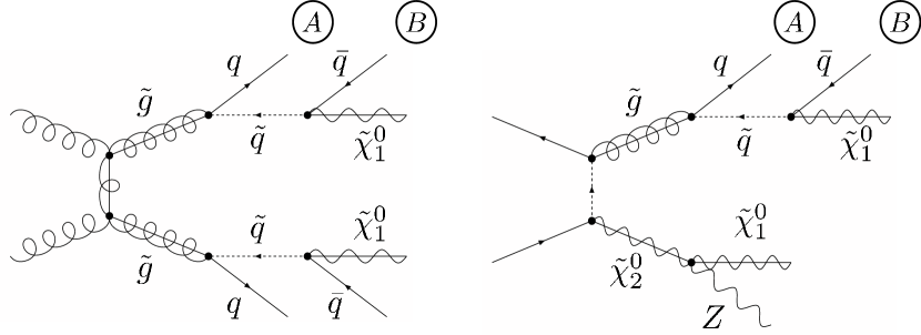
As examples, we consider two processes in a supersymmetric theory with squarks and a gluino with : associated production of and and same-sign squark production, as in Figure 2. The squark decays directly to a quark and the LSP, while the gluino decays through an off-shell to two quarks and the LSP. The full quantum amplitudes for these processes depend on many Lagrangian parameters of the MSSM. The OSET description of Figure 3 is, however, very simple—there are three new particles , , and LSP, two production modes, and two decay modes. We emphasize two features of the OSET description. Though the same-sign squark production amplitude depends on the gaugino spectrum, the gauginos do not appear on-shell anywhere in this process, and are excised from the OSET description. In SUSY associated production, the squark appears both on-shell (directly produced) and off-shell (in gluino decay); the OSET analogue keeps the squark where it appears on-shell, and “integrates it out” where it is off-shell.
As we will show in Section 2 and the appendices, OSET production and decays can be simply and accurately parameterized with no more than an overall (integrated) cross section and, in some cases, one or two “shape” variables. This simple parameterization reproduces features such as the locations of invariant mass edges and endpoints, and in most cases the locations and widths of peaks in distributions. In our figures, we represent the parameterized components of amplitudes as shaded circles, or “blobs”. More or less detail can be incorporated as appropriate, for example the addition of spin correlations or simplification of cascade decays into a single blob.
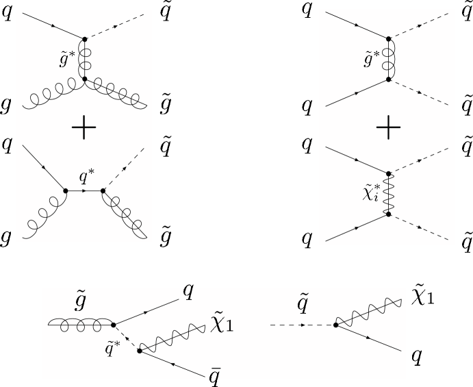
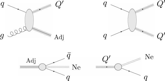
An OSET that describes a particular topology of production and decay will almost always make predictions for the existence and relative strengths of other topologies. Thus, a consistent picture is tightly constrained. The OSET has transparent physical meaning. An OSET that fits the data well will strongly constrain the structure of the underlying new physics, and a model inspired by the OSET can suggest new channels to be be included in a refined OSET description. Thus, the OSET framework allows us to describe the new physics in stages rather than getting the full effective Lagrangian in one go. Consistency with an underlying Lagrangian also implies basic guidelines that should be considered throughout the process of interpretation—for example, a 1 TeV weakly interacting particle should not be produced with pb cross section! As this feedback loop converges on a model or set of models for new physics, detailed simulation may be required to verify features that are not incorporated in the OSET.
1.3 Inclusive Data Analysis with OSETs
With a well-defined OSET parametrization scheme in place, the field is open for applying powerful analysis techniques to OSET-based searches and data characterization. We fully expect that the experimental community will be adept at analysis; our remarks here and in Section 4 are intended to illustrate potential benefits of OSET-based analysis, not to advocate a particular analysis strategy.
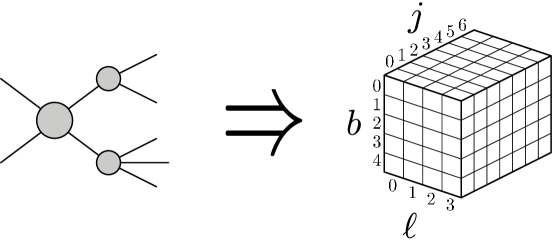
Compared to Lagrangian parameters, OSET parameters are relatively easy to extract from data. Object multiplicities and the shapes of kinematic distributions motivate a set of OSET diagrams. Approximate mass scales can be inferred from standard kinematic distributions, and a simple set of inclusive signatures—for instance counts for leptons, jets and -jets binned in ranges as in Figure 4—constrain cross sections and branching ratios [21, 22, 23, 24]. These signatures should be supplemented with more carefully designed discriminators to distinguish processes with similar topologies from one another and from Standard Model processes. An OSET will populate this space of final states with a particular pattern; a pattern in the data not captured by the OSET then suggests new “blobs” to be included in a better OSET description. In practice, this process has been most effective on examples when the OSETs are well-motivated by top-down theory considerations. As a first step towards designing more sophisticated analysis techniques, we show that OSET parameters can be determined by crude but effective Mass And Rate Modeling (MARM) analysis techniques, shown schematically in Figure 5. This will be the main topic of Section 4 using the “Michigan Black Box” as an example.
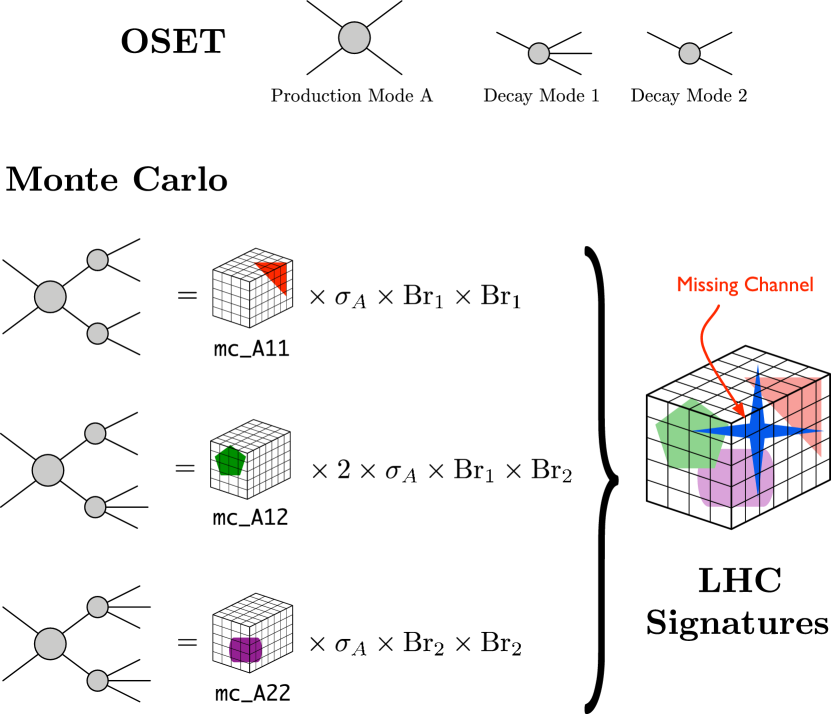
We have implemented OSET-level Monte Carlo generation in a Pythia-based [25] analysis package called MARMOSET, described in detail in Section 3 and available for download at http://marmoset-mc.net/. MARMOSET is a Monte Carlo tool allowing direct simulation of OSETs for new physics, in place of an effective Lagrangian. The machinery to Monte Carlo such models has been available in event generators for years. What has been missing is an interface for simple specification of OSETs with minimal vertex structure and for bookkeeping of rate correlations. The organization of Monte Carlo in MARMOSET allows efficient comparison of OSET hypotheses to Hadron Collider data.
We use this in the simple analysis of Section 4. This strategy is analogous to the template method familiar from top mass measurements [26], but focuses on gross observables, explicitly treating kinematics and rates independently. In principle, best fit OSET parameters can be obtained through a simultaneous fit to signal and various background channels weighted independently, reducing the possibilities of “fake” discoveries through background normalization errors. Of course, the optimal analysis path will depend on the details of the new physics, the important backgrounds, and detector resolution.
Because Monte Carlo generation and detector simulation are time-consuming, MARMOSET is organized to exploit the economy of OSETs for computational efficiency. This economy is achieved through two simplifications. In the underlying Lagrangian description, rate variables are strongly dependent on masses, so that a high resolution in scanning many masses is needed to adequately scan rates. By separating rate information from masses and rendering masses of off-shell particles altogether irrelevant, OSETs greatly reduce the dimensionality of parameter space and the resolution required in mass scanning; crude mass estimators can often be used to approximately fix mass scales without compromising the accuracy of branching ratio and cross-section fits. Moreover, because the Monte Carlo for different processes is additive and rates are floating parameters, these rates can be varied without re-generating Monte Carlo by simply re-weighting events.
As discussed in Section 3.6, this MARMOSET analysis strategy is analogous to that taken in Bard [27, 28], while the organization of the physics characterization is complementary. MARMOSET is aimed at the problem of characterizing mass scales and rate correlations among many competing topologies, mainly with LHC scenarios in mind. Bard approaches the problem of characterizing new physics by systematically generating and evaluating Lagrangian explanations of discrepancies.
1.4 SUSY Examples with OSETs


The need for an intermediate characterization of new physics becomes clear in attempting to solve “black box data challenges”; we illustrate the use of OSETs in this context. A “black box” is a simulated data set for some theory of new physics—unknown to us—with of integrated luminosity at the LHC. The simulations are done as realistically as reasonably possible, with fast detector simulation and in some cases relevant Standard Model backgrounds included. The “data challenge” is to determine the underlying model from the “black box” data. In all examples, unsophisticated analysis of simple kinematic distributions allow us to build OSETs that, in turn, guide us rapidly to the “right” TeV-scale Lagrangian, often in surprisingly interesting ways.
We begin with two SUSY examples for which the general structure of the theory is already widely familiar. The first example is the supersymmetric “Michigan Black Box” [29]. The spectrum of this model is shown in Figure 6; the dominant production and decay rates are shown in Figure 8. The spectrum is evidently unconventional, with a very heavy Wino, a light gluino and a Higgsino LSP. The top and bottom squarks, which mediate gluino decays and so are essential in a renormalizable field theory description of the LHC signals, are produced with tiny cross-sections , so their properties are not directly measurable. In the absence of electroweak cascades, the LSP identity is difficult to ascertain. Thus, the MSSM Lagrangian is complicated and is impossible to deduce experimentally. As we show in Section 4, however, the OSET description found in Figure 7 is quite simple. Moreover, the OSET fit we have obtained from limited signal information, as illustrated in Figure 8, demonstrates a striking agreement between OSET and model.
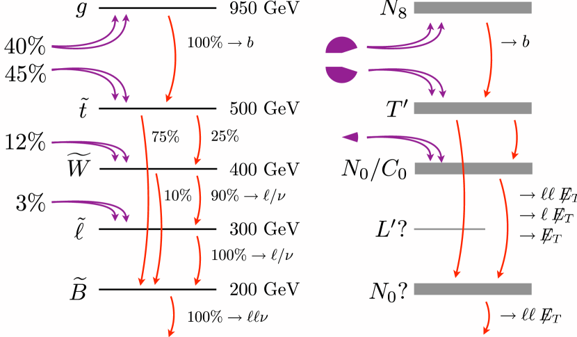
Though the “Michigan Black Box” was peculiar from a theoretical perspective, it was dominated by a small number of production and decay modes; the advantage of an OSET parameterization is in representing these few processes more simply. OSETs are also useful in describing models with numerous production modes and more complicated decay topologies. This is illustrated by our second SUSY example, the model of Figure 9, and its accompanying OSET. The underlying theory is a supersymmetric theory with R-parity violation, the “Rutgers Black Box” [29]—the absence of certain details in the OSET (e.g. the on-shell slepton) reflects the difficulty of resolving this aspect of the physics in the first stages of analysis with only 4 fb-1.
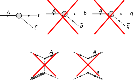
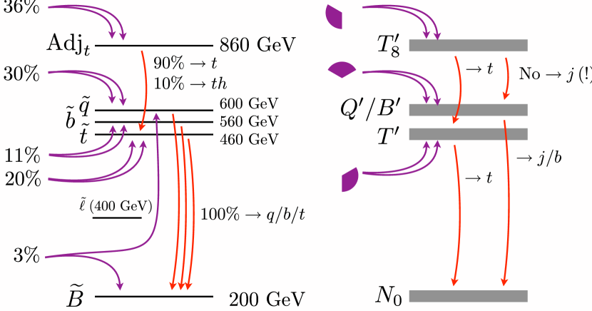
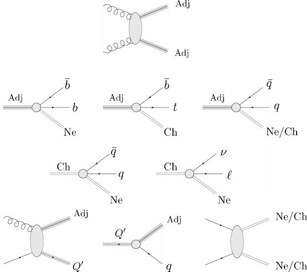
Our third example is another supersymmetric model, but with a twist. Suppose that gauginos are very heavy, say all heavier than TeV, so aren’t directly produced at the LHC, while the scalars are light and accessible as usual. However in addition, there are light chiral superfields in the adjoint representation of the standard model; this can easily occur in a wider variety of well-motivated theories of SUSY breaking. In particular there is colored adjoint field . The only way this particle can decay is via higher-dimension operators in the superpotential of the form where the , are Standard Model fields. Since these couplings are necessarily flavor violating they are naturally largest for the top so the leading decay is via the operator . Let’s suppose that is heavier than both the third generation as well as first-two generation squarks. Then the leading decays are , as well as a three-body decay to .
A simple rate analysis of the signal isolates three production and decay modes, all consistent with a garden-variety MSSM: pair-production of colored adjoints and of colored triplets decaying to the third generation as well as first two generation jets. The surprise is in the preferred branching ratios for adjoint decays in the OSET—though they are kinematically allowed, decays to the first two generations are absent or highly suppressed as in Figure 10. This colored adjoint can’t be a usual gluino! This interpretation is further confirmed by the absence of an adjoint-triplet associated production mode, and by the production cross-section for Adj, which is consistent with QCD production through an -channel gluon, but is missing the expected -channel contribution from the first-generation squark.
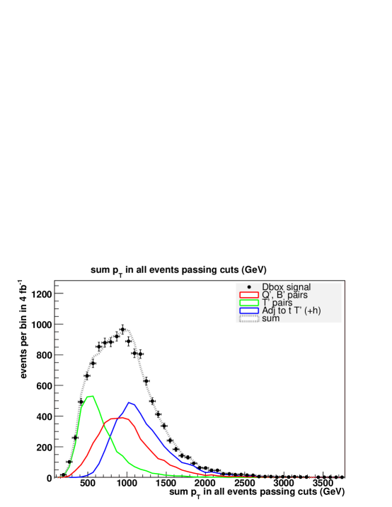
The peculiar properties of the OSET immediately suggest the central interesting feature of the underlying model—that the colored adjoint is not a gluino but a new field decaying through a higher-dimension operator! In turn, this model suggests an additional channel for the decay of the adjoint—the three body decay also including the Higgs, that can be added to the OSET and searched for. Indeed, even with fb-1 of data, there are hints for this rare decay in events with many jets + . The final OSET fit to this theory, again with the zeroth order approximations to production and decay, is shown in Figure 11. Again, the agreement is striking, and the OSET description in Figure 12 is a clear characterization of the physics.
1.5 OSETs at the Energy Frontier
The above examples illustrate that when faced with signal, attempting to describe hypotheses in the OSET language of particle production and decay modes is second-nature; the ability to verify hypotheses at this OSET level dramatically simplifies the interpretation process. As we will argue in Section 4, an OSET description is readily attainable once the new-physics signal has been isolated from Standard Model background. This OSET is determined using simple shape and object-multiplicity observables, analyzed with theoretical constraints and prejudices in mind.
Certain aspects of data analysis can and should be automated, including the generation and testing of hypotheses. At the same time, the development of the “big picture” needs a human operator to guide it. In the examples above, the initial guesses for the OSET structure are made by a global survey of gross features of the data, using relatively simple tools. The interpretation of these results involves guesswork and theoretical intuition, allowing humans to do what humans do best—recognize broad patterns and make models. MARMOSET organizes the “grunt work” of simulating arbitrary hypotheses and comparing them to data.
MARMOSET represents a coarse-grained approach to LHC signal interpretation. The ability to accurately simulate general, complete Lagrangians is clearly also important, and tremendous progress has been made in implementations such as Bridge [30], CompHEP [31]/CalcHEP [32], Grace [33], Herwig [34], MadGraph [35], Pandora [36], Sherpa [37], and Whizard [38]. An interface between MARMOSET and these tools would also be useful. In the opposite direction, Bard can be further developed as an automated tool for searching through tree-level renormalizable Lagrangians matching excesses. A successful Lagrangian characterization may be derived from the top down or from the bottom up, and will be most convincing if understood in both ways.
2 The Physics of On-Shell Effective Theories
An OSET is a description of new physics processes in terms of just on-shell particles. The kinematics—masses and phase space—of production and decay vertices are treated exactly, while the highly model-dependent dynamics appearing in quantum amplitudes are approximated using a simple parametrization of . In this section, we develop this broadly applicable parametrization for dynamics, and show that it accurately reproduce a large class of observables. The behavior of parton distribution functions (PDFs)—and in some cases the inability to fully reconstruct events with missing energy—will facilitate this task immensely.
Of course, the complexity of the parametrization required depends on the desired accuracy; our goal is to enable the self-consistent determination of an OSET from new physics signals. We will argue in Section 4 that relatively uncorrelated observables, such as single-object ’s, , distributions, and object multiplicities, are sufficient to shed light on the topology of new physics processes as well as constrain mass differences and rates. Therefore, these are the distributions we will try to reproduce faithfully. A useful OSET must also reproduce rapidity and relative angular variables on which data is frequently cut to reduce Standard Model backgrounds, so that the sculpting of new physics distributions by these cuts is reasonably modeled. In this discussion, where no detector simulator is used, we will use the rapidity of a hard object in the lab frame as a proxy for the reconstructed detector on which cuts are applied.
We consider production dynamics in Section 2.1, and introduce a leading-order parametrization for hard scattering matrices. The brief discussion here is supplemented by a more thorough one in Appendix A. After introducing an expansion for in production in Appendix A.1, we note useful approximate factorization/shape-invariance results in Appendix A.2, and demonstrate analytically the PDF-suppression of the higher-order pieces in our expansion in Appendix A.3. In Appendix B, we present a large number of examples illustrating the success of the two-parameter models of considered in this section.
Decay dynamics are discussed in Section 2.2 and elaborated upon in Appendix C, where we find that some care must be taken in interpreting di-object invariant mass distributions in an OSET framework. On the other hand, because the axis of the initial production has been lost, single object distributions are reproduced with reasonable accuracy by decaying particles simply via phase space. These discussions of production and decay dynamics provide the theoretical foundation for Section 2.3, where we give a definition of an OSET suitable for the Monte Carlo program we introduce in Section 3.
We will see that dynamics play a secondary role to kinematics in predicting LHC signatures, such that precise modeling is less important than gross structural properties. The reasons are that long decay chains wash out detailed correlations, low luminosity measurements have insufficient statistics to resolve theoretical shape differences, and detector effects smear out all distributions.
Having emphasized the importance of kinematics over dynamics, a caveat is in order. The degree of coarse-graining appropriate to an analysis is determined by experimental resolution—i.e. data set size, detector performance, understanding of Standard Model backgrounds, and the whims of a given experimentalist. In some cases, kinematics are not completely resolvable, while in others it may be desirable to include more detailed dynamics in matrix element structure for production or decays. Though we will focus on the middle ground of accurate kinematic modeling and coarse dynamic modeling, the MARMOSET tool we develop in Section 3 is organized in anticipation of a progressive analysis that interpolates between approximate OSETs and actual Lagrangians.
2.1 Particle Production Without a Lagrangian
Our first goal is to develop a parametrization scheme for describing particle production at a Hadron Collider when we have no, or only partial, information about the underlying theory or Lagrangian. The production and decay of a single, narrow resonance () is fully specified by the resonance mass , production cross section , the branching ratio to the final state of interest, and a finite polynomial in determining the angular distribution of decay products.
It is clear that no such exact, finite scheme exists for parameterizing non-resonant production. These processes must be described over a finite range of partonic center-of-mass energy, so full dependence is important. Also, -dependence doesn’t truncate at finite order as evidenced by a -channel propagator that yields an infinite power series in . Both -dependence and angular dependence of would have to be expanded in infinite series to capture the full matrix element.
| Particle | Mass (GeV) |
|---|---|
| 992 | |
| 700 | |
| 197 | |
| 89 |
Rather than a power series, we could use tree-level field theory to constrain the form of matrix elements. For example, in Figure 13 we illustrate gluino pair production through the gluon PDFs [39], which has the matrix element [40]
| (1) |
with , . There is also a contribution from a initial state
| (2) |
with () dependent on the squark mass. Within a given model, both expressions involve a finite number of pieces, and we can add terms appropriate to different spin possibilities. But the choice of matrix element depends on, say, knowing how many states can propagate in the -channel, and one must specify all of their masses to parameterize the matrix element fully.
There is reason to hope, however, that hadronic production is insensitive to the details of this structure. The matrix element varies smoothly over energy, whereas parton luminosities fall rapidly about threshold. The kinematics of the gluino pair-production process of Eq. (1) is quite well reproduced by the truncated expression
| (3) |
with a value chosen to reproduce the total hadronic production cross section. Of course, this constant has no Lagrangian interpretation, but it serves as an effective leading order parametrization for various kinematic variables. The and rapidity distributions for a gluino produced according to the full matrix element of Eq. (1) and the approximation of Eq. (3) are shown in Figure 14. The agreement is striking! The distributions for a visible decay product have been convolved with decay kinematics, and are even less sensitive to detailed production dynamics.



The success of this approximation relies dominantly on the approximately polynomial fall-off of parton luminosities. When the most naive constant approximation fails, it does so for the clear, physical reason that the threshold- or high-energy scaling of is extreme in one limit or the other. For example, -wave scattering amplitudes vanish at threshold, and four-fermion contact interactions grow up to a cutoff scale ( is the threshold scale). In parameterizing corrections to constant , it is convenient to introduce dimensionless energy and angular variables related to the Mandelstam parameters , , and of the hard subprocess. We define
| (4) | |||||
| (5) |
where is the minimum possible value of (for production of species of masses and , ),
| (6) |
is the relative velocity of the products, and is the scattering angle in the center-of-mass frame. The variable is the -component of momentum of the particles in the center-of-mass system scaled by half the center-of-mass energy.
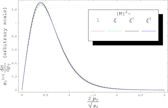
In this basis, parameterizations that reproduce distributions simplify remarkably because and produce nearly identical shapes. This equivalence is exhibited in one example in Figure 15, but is quite general and will be discussed further in Appendix A. Though -dependence does affect final-state rapidities, the leading term usually dominates. Moreover, PDFs and cascade decays tend to wash out effects on individual decay product rapidities, as discussed further in Appendix B. If events cannot be fully reconstructed, and distributions matter mostly for their systematic effects on analysis cuts, modeling by a function that depends only on is sufficient. Motivated by extreme scaling behaviors of with center-of-mass energy, we will try to find a small but sufficient basis for parameterizing -dependence.
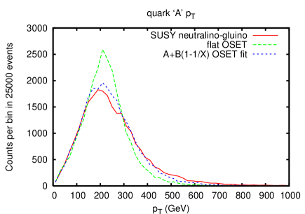
As an example of threshold-suppressed production, we consider the associated production process in the model of Figure 13. Unlike gluino production, it is -wave dominated and near threshold. As shown in Figure 16, a flat ansatz does not reproduce the gluino decay product . The function reproduces this threshold behavior (for , ), and a linear combination
| (7) |
with and obtained by a fit reproduces the SUSY distributions quite well in Figure 16. We emphasize that the and that reproduce overall rates and distributions are not the coefficients one would find in a Taylor expansion of ! Rather, because of the shape invariance of the transverse structure, the coefficients and are only an effective parametrization after integrating over PDFs. The term in this case arises from pieces in the underlying matrix element.

When , displays qualitatively different energy scaling. Integrating out the -channel squark, we see that at energies well below , the interaction is modeled by a four-fermion operator, with . This growth of is, of course, cut off for , but PDFs will cut off the distributions, anyway. With contact-like interactions, a good fit to ’s is achieved with
| (8) |
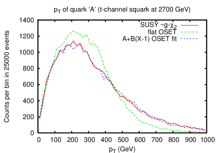
For -channel intermediate squark mass TeV, the results of constant and linear parameterizations for are shown in Figure 17; we note that is quite small, contributing to the total cross-section. At higher squark masses (where the cross-section for this process is also lower), a quadratic term may be added for a more accurate fit.
This example illustrates another reason that simple matrix elements are often quite effective: when decay products are boosted, their relative in the rest frame of the parent particle washes out inaccuracies in modeling of the distribution of this parent particle. For instance, whereas misestimates the gluino by nearly a factor of 2 in Figure 17, the of a quark into which it decays is only inaccurate at the level.

Although angular dependence is the only important structure of in the resonant production case, we have said nothing about its role in non-resonant pair production. Indeed, we achieved a good fit to and in the previous example by fitting a function of , when is manifestly a function of . In Appendix A.3, we note the striking result that, when integrated over PDFs, distributions are independent of the -dependence of to a very good approximation. Moreover, modeling shape with has little effect on the rapidity distribution , which is controlled dominantly by PDFs and secondarily by the -dependence of . Therefore, the problem of modeling ’s and ’s is largely factorizable; in practice, if events cannot be fully reconstructed and one seeks only to reproduce single-object and lab-frame distributions, -dependence of the amplitude can be ignored.
Deviations from this factorizable structure will give rise to theory systematic errors; for example, the -dependent parameterization of obtained by fitting to momentum distributions of central objects differs from what one would expect from theory if all events were treated equally. Therefore, when using the approximate parametrization method, experimentalists should be aware of these systematic effects, and try to estimate them.
Then again, the theory systematics of different parametrizations for are not very different in magnitude from the kinds of theory systematics one encounters in comparing LO and NLO results for a given theoretical model. In the context of a model with real matrix elements, the largest NLO systematic is on overall normalization, whereas in an OSET parametrization, the total cross section is a free parameter that is matched to the data anyway. The advantage of a OSET parametrization is that systematic effects reflect our actual uncertainty about the underlying model while still allowing quantitative comparisons between models and data.
Finally, in some cases, production modes can be key to discovery of new physics. Notable examples include vector boson and top fusion in production of Higgs-like resonances. In these examples, Standard Model dynamics has enormous effect on event shapes, but new physics internal lines are absent. Extending the matrix elements for Standard Model Higgs production to more general new physics scenarios is a reasonable approximation; we will not discuss it further.
2.2 Decay Kinematics and Final State Correlations
So far, when presenting and rapidity distributions for decay products, we have assumed that all decays are weighted only by phase space. In this section, we examine the structure of more general decays matrix elements, and their effects on variables of interest. Though the current implementation of MARMOSET only allows for phase space decays, we discuss systematic ways of including these effects and improving our approximation.
We choose to focus on single- and two-object observables that are relevant to determining the gross structure of a model and could be measurable with low luminosity—’s of single objects (or uncorrelated sums of several of them) and pairwise invariant masses such as are useful variables for characterizing decay chains, is frequently employed in cuts to reduce Standard Model background, and object ’s are used both to determine signal acceptance and background reduction. Though invariant mass observables involving more than two objects can be useful [41], interpreting them will probably require higher statistics and we will not discuss them here.
Correlations in the rest frame of a decaying particle tend to be washed out after boosting to the lab frame. For this reason, when events cannot be fully reconstructed, the phase space approximation reproduces single-object and distributions quite well. Spin correlations do induce observable effects on distributions of decay products, such as the lepton in top quark decay. Such effects can be exploited for precision analysis (for example, the determination of helicity and top polarization in top decays [42, 43, 44, 45]), but are subleading for discovery.
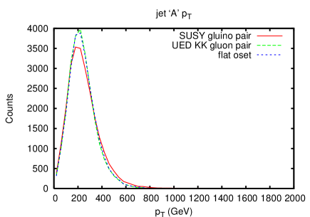
Inaccuracies in would lead to systematic errors in measuring the cross section of new physics when cuts are used to remove QCD background from searches for new physics in hadronic channels. In principle, the directions of a jet and the missing particle in the same decay chain are correlated. But averaging over both decay chains in makes this variable fairly insensitive to spin correlations. Partonic distributions for SUSY, UED, and OSET processes with the same topologies are visually identical (see Figure 63, again for the pair-production process).
Next, we discuss the distributions of invariant mass observables. We should stress that phase space, together with on-shell conditions, reproduces positions of kinematic end-points, but do not reproduce their shapes. Unlike the transverse variables, invariant mass distributions are invariant under the boost to the lab frame, and spin correlation information is not diluted. Exploring such information to measure spin has been studied recently [46, 47, 48, 49, 50, 51, 52, 53, 54, 55, 56].
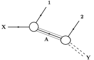
Factors that can change the shape of the invariant mass distribution significantly include, spin correlations, effects of off-shell propagators, as well as interference between several processes. We consider the decay process shown in Figure 18. We can systematically improve our approximation by expanding the differential decay width in a single pair’s invariant mass as
| (9) |
Keeping only corresponds to our original flat matrix element approximation.
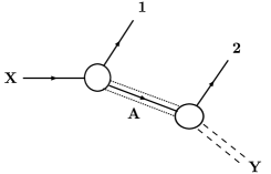
We begin by considering the case that the intermediate particle is on-shell. In this case, we can consider a single channel shown in Figure 18 since interference effects are typically small in on-shell decays. In this case, the shape is almost completely determined by spin correlations. In particular, the degree of the polynomial satisfies [54], where is the spin of the intermediate particle . Constants depend on the masses of particles in the decay chain, the chiralities of the couplings, and the masses and spins of final-state particles and . If, for instance, is fermion, the sign and value of depends on whether and/or are vector or scalar, as well as mass differences such as [56].
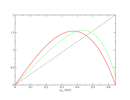
The dependence of the parameters on masses demonstate perfectly the need to characterize mass hierarchies before extracting spin information from decays. But particularly when decays can be cleanly isolated (e.g. di-lepton invariant masses), the cannot be forgotten. An edge that appears clearly in an OSET with the correct spectrum may be invisible in the data if angular momentum conservation forces the distribution to vanish at the edge! If both and are scalars, angular momentum conservation force the distribution to vanish exactly at the edge as in Figure 19. In other cases correlations may reduced the edge so much that we cannot tell it apart from statistical fluctuations [48]. For comparison, we have also included a UED-like case where the intermediate particle is a vector and and are fermions. Given fluctuations and combinitorics, it will be challenging to resolve the end point structure of the solid curve. Therefore, the absence of an edge in the data should not rule out an OSET—it should instead warrant of a thorough study of the dependence of Eq. (9).
|

|
When an intermediate particle is off-shell, is modified by both spin correlations and the momentum-dependence of the propagator, which is more significant when the intermediate state is close to on-shell. Both deformations can be parameterized by a polynomial in . So long as we consider only a single pairwise invariant mass distribution, the presence of multiple decay modes as in Figure 20 and the resulting interference can also be modeled by a polynomial in . This improved treatment of decay matrix elements based on Eq. (9) is particularly useful in the cases when an OSET analysis reveals a large deviation in invariant mass distributions while other observables show good fits.
A qualitatively different case is when a new resonance decays into several visible Standard Model particles, allowing full reconstruction and facilitating spin determination. More complete angular information in the rest frame of the decaying particle would have to be included. For instance, in a two body decay, angular information could be systematically included by expanding . Conservation of total angular momentum restricts the allowed values of .
2.3 Definition of an OSET
The preceding discussion allows us to define an OSET more precisely than the preceding intuitive descriptions. It is specified, first, by a spectrum of new particles with given masses and possibly observable widths (if instrumental widths dominate, unknown physical widths can be set to arbitrarily small values). Though not strictly speaking necessary, the and gauge quantum numbers for new particles are also specified, both for reasons of theoretical consistency as well as to enable OSETs to be simulated using Monte Carlo tools like Pythia that model initial/final state radiation and parton showering.
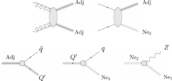
The remaining content of an OSET concerns the observable production and decay modes, in terms of only the particles that appear on-shell in each mode. For example, the processes of Figure 13 would be described by an OSET containing the production and decay elements shown in Figure 21. Each OSET vertex is represented by a gray blob, which reminds us that we are choosing an approximate, parameterized matrix element . The type of structure depends on the context in which a blob appears (e.g. production vs. decay) and the amount of structure is chosen such that terms that do not produce resolvably different observables are not included. In practice, more detail is required in modeling production than decay.
In our leading-order OSET parameterization, the blob structures are as follows:
-
•
Resonant Production from a given partonic initial state is specified by an overall hadronic cross section, integrated over the appropriate PDFs. Together with the mass and width of the resonance, this fully determines the resonance production from unpolarized initial states. In this case, it is possible to extract from the hadronic cross section and PDFs a partonic cross section, and from this a squared coupling. This near-equivalence between an OSET process and a renormalizable Lagrangian is particular to resonant production, and not generic. Of course, without specifying the decay modes of the resonance, observables such as forward/backward asymmetries will be lost.
-
•
Pair or Associated Production from a given partonic initial state can typically be approximated by
(10) The two forms are appropriate for threshold-suppressed and contact-like interactions, as discussed in Section 2.1. When a term is needed to match distributions, the preferred form is usually clear from the shape of the tail. In many cases—production of heavy particles of comparable masses, with poor statistics, or in generating exclusions on processes that have not been observed—a parameterization in terms of alone is most useful. In cases of high-precision measurement, the expansion can be readily expanded to include higher powers of and/or leading -dependence (this could be linear or quadratic, depending on symmetries). We refer the reader to Appendix A for more detailed discussion of matrix element structures.
As free rate parameters for production, we can use either the partonic and or the more directly observable PDF-integrated hadronic cross-sections for each term. If and are used, the OSET expression for looks like an effective Lagrangian, but it cannot be interpreted as such— is not the coefficient of in an effective Lagrangian, but a linear combination of coefficients for -dependent contributions to . For example, -wave production does not mean that , but only that the dominant contribution to has non-trivial -dependence.
-
•
Production is typically very far from uniformly filling out phase space. For example, in weak boson fusion into a Higgs, the scattered quarks are typically quite forward, and we can think of the Higgs as being resonantly produced from off-shell weak bosons. Thus, Standard model dynamics affects phase space considerably, whereas the dynamics of new physics is quite simple. The same is true of production, though this includes radiated Higgs production from off-shell top quarks in final states. In our current implementation, we will only include these two classes of production in OSETs, with the same dynamics as for the Standard Model Higgs processes. Such processes would be characterized by one overall rate. For most intents and purposes, processes with two new particle final states and one QCD jet are adequately described by production with parton showering.
-
•
Decay is modeled at leading-order by constant. This is currently the only decay incorporated in MARMOSET. Two simple situations require more detail: if the decay is of a singly-produced resonance or if events can be fully reconstructed, it may be desirable to incorporate angular dependence. Likewise, angular and (for three-body decays) energy dependence may be needed to reproduce the shapes of kinematic edges and endpoints. The ability to handle the decay parameterization of Eq. (9) will be added to future versions of MARMOSET.
When total decay widths cannot be measured, only products of branching fractions and cross sections are observable. However, when more than one process has been observed, it is often easier and instructive to parametrize rates in terms of branching fractions instead of overall rates for individual processes. This is because branching fractions properly account for combinatoric factors in decays, so correlated final state multiplicity information is retained. This is the MARMOSET default.
We note that in this parameterization, spin is not explicitly included. Nonetheless, non-trivial matrix elements for various processes can incorporate the leading effects of spin on threshold behavior and angular distributions.
Now that we have defined an OSET parametrization, we have a choice for how to generate OSET Monte Carlo. We can imagine two ways of implementing a production matrix element with unknown and . Currently in MARMOSET, one generates separate samples with 1 and , and mixes them together with appropriate weights. Though simple, this approach does not generalize well to more complicated expressions, particularly if the formulas in question are not additive. A more robust alternative is to generate and simulate Monte Carlo for a flat matrix element, keeping both detector-simulated event records and partonic kinematic information. Then, a given choice of and determines a weight associated with each event. These weights can be stored, or events can be unweighted by keeping only those that satisfy for a random number . The difficulty with this method is that unweighting can be extremely inefficient for certain matrix elements. In practice, we imagine that some combination of preweighting and reweighting will be the most efficient use of OSET Monte Carlo.
The matrix element parameterizations we have outlined are useful when we are in the dark about the underlying physics. One would hope, however, that an OSET analysis (to be discussed in Section 4) combined with theoretical understanding will quickly lead us to a correct framework for describing the new physics observed at the LHC. In this case, a parameterization in terms of on-shell masses and the efficient process-by-process Monte Carlo generation that it permits will continue to be useful as an efficient means of scanning parameter space, but naive rate parameterizations will have outlived their usefulness. In this scenario, it may well be more reasonable to parameterize dynamics through a full set of model parameters, sliced into surfaces of fixed masses for species produced on-shell. As one moves along such a slice, changes in can be incorporated by re-weighting of saved Monte Carlo as discussed above.
The converse situation can also arise, in which an OSET contains too much kinematic detail. When mass ratios are neither very large nor very small, on-shell particle masses may not be clearly resolvable and it may not be clear which states in a decay chain are on-shell. It may then be useful to parameterize a chain of decays as a single decay, as in Figure 22. This is readily done in an OSET framework.

3 MARMOSET: A Tool for OSET Monte Carlo
The OSET parametrization introduced in the previous section allows us to describe a wide class of TeV-scale models quite simply, in terms of the masses, quantum numbers, production modes, and decay modes of new particles, at the level of cross sections and branching ratios. We have seen that even with leading-order coarse approximations, an OSET reproduces single-object kinematics and some features of correlated kinematic variables (edge and endpoint locations in invariant masses) with reasonable accuracy, and a more detailed correspondence can be achieved systematically. One key feature of an OSET is that mass parameters that affect kinematics are disentangled from the specification of rates for new physics processes. In this way, an OSET can be simulated additively process by process. In this section, we introduce MARMOSET (Mass and Rate Modeling in On-Shell Effective Theories), currently a Pythia-based tool for generating Monte Carlo for any model that is well characterized by a finite set of particles. More information about installing and using MARMOSET can be found at http://marmoset-mc.net.
MARMOSET manipulates Pythia’s behavior in two ways: we have extended Pythia’s production modes to include parameterized production of the kind described in Section 2.3, and we have built a user interface and organization scheme for generating separate Monte Carlo for individual decay topologies while keeping track of the appropriate relative weightings. Thus, MARMOSET provides a straightforward means of event generation for a broad variety of models for which no full Monte Carlo implementation exists. Development of an alternative MadGraph/MadEvent [35] back-end for MARMOSET is ongoing, and it would be straightforward to modify MARMOSET to interface with other Monte Carlo tools.
For studying single topologies, MARMOSET can generate exclusive processes that can be used for setting experimental limits on the overall rates as functions of the physical mass scales involved. For studying correlated topologies, MARMOSET allows for an efficiently scanning of production cross sections and branching ratios even when this scanning demands consistency relations between the rates for different processes. This is accomplished by reweighting Monte Carlo events after they are generated. A simple analysis technique that makes use of the property will be discussed in Section 4.
Currently, MARMOSET simulation of a new physics model is achieved in three steps:
-
1.
To simulate an OSET, a user specifies the masses and and quantum numbers of new particles, as well as their production and decay modes. The specified production and decay modes are sewed together in all possible ways to generate a list of consistent topologies. Each topology is assigned a weight function , where numerical values of and will be determined through later analysis. The production matrix elements can be specified using the leading-order parameterization of Section 2.3. In the current implementation, decays always proceed according to phase space.
-
2.
Monte Carlo events are generated separately for each topology. StdHEP and PGS4-simulated output are currently supported. This stage is highly parallelizable. Exclusion limits on for a given topology can be set directly using the Monte Carlo for a single process. For each topology, Monte Carlo is implemented by creating a special-purpose branching ratio file in Pythia native format.
-
3.
The appropriate weights for each topology are uniquely determined by specifying hadronic cross sections for each production mode and branching fractions for each decay mode and the individual Monte Carlo can be readily combined. Alternatively, each process can be treated as a template with a constrained rate, and an optimization technique can be used to quickly find the “best fit” values of OSET rate parameters. A simple version of this approach is illustrated in Section 4.
In the following subsections, we describe the input format and give more details on the workflow for Monte Carlo generation.
3.1 Building a Simple OSET
The process of building an OSET input file is best illustrated by example. A new with a mass of 900 GeV and a width of 50 GeV would be specified as:
Zprime : charge=0 color=0 mass=900.0 width=50.0 |
(11) |
The variable charge specifies , and color is 0
for a color singlet, 3 () for a color (anti-)fundamental,
and for an adjoint. Note that the spin of the is ignored,
but we plan to add spin-related correlation functionality in future implementations. We
have not yet given MARMOSET production or decay modes for the ,
which we do as follows:
u ubar > Zprime Zprime > e- e+ |
(12) |
The first line defines production of from and PDFs using a Breit-Wigner parametrization, while the second line permits decays to . MARMOSET knows about these Standard Model particles from definitions such as:
u ubar : pdg=2 charge=2 color=3 mass=0.33 e- e+ : pdg=11 charge=-3 color=0 mass=0.00051 |
(13) |
The pdg code is the Particle Data Group’s standard Monte Carlo reference number [57]. Note that the charge, color, and mass
specifications are used by MARMOSET to check consistency, but Pythia standard values are used in Monte Carlo generation.
# Standard Model Particles u ubar : pdg=2 charge=2 color=3 mass=0.33 e- e+ : pdg=11 charge=-3 color=0 mass=0.00051 # New Particles Zprime : charge=0 color=0 mass=900.0 width=50.0 # Decay Modes Zprime > e- e+ Zprime > u ubar # Production Modes u ubar > Zprime
# Processes p001 * s1 b1 $ u ubar > (Zprime > e+ e-) p002 * s1 b2 $ u ubar > (Zprime > u ubar) # Rates s1 = 1000 $ Sigma( u ubar > Zprime ) b1 = 0.5 $ Br( Zprime > e+ e- ) b2 = 0.5 $ Br( Zprime > u ubar ) @ b1 b2
There is a crucial difference between OSET vertices and Lagrangian vertices: even though the can be produced by , it does not necessarily need to decay to . An OSET is organized with experimentally resolvable branching ratios in mind, so only if the decay channel is visible would the user be interested in adding this mode. Adding it to the OSET is simple using:
Zprime > u ubar |
(14) |
The two processes and will be generated independently, so the OSET input file does not need to supply any coupling strength or rate information.
Using the complete input file from Figure 23,
MARMOSET constructs two processes p001 and p002 shown
in Figure 24. Between the index
(pXXX) and the $ sign is the rate formula for each
process in terms of the overall cross section s1 and two
branching ratios b1 and b2. The rate parameters are
listed alongside default values which can be changed by the user.
The @ symbol indicates which branching ratios are constrained
to sum to 1. Since , there are two free
rates, one for each process. This counting always holds for
resonant production with decays to the Standard Model. For longer
decay chains, there are typically more processes than free
parameters, and correlations between the process weights are
important.
3.2 Pair Production and Stable New Particles
Let us add to our OSET a new process, perhaps to account for an
observed 4 jet missing excess. The syntax is given in
Figure 25. We have added a neutral particle
and a color adjoint particle . The new
particle Ne is stable, so we give it a pdg number
1000022, so that it is properly interpreted as a stable, neutral
particle by detector simulators.222In the current
implementation, there can only be one kind of neutral stable
particle and it must have pdg=1000022. In a future
release, the user will be able to define arbitrary “stable”
particles by assigning them non-zero pdg numbers, and it
will be the users responsibility to make sure those particles are
handled properly by Pythia and detector simulators. The new
particle Adj can be pair produced through and has two decay modes
and
.
# More Standard Model Particles g : pdg=21 charge=0 color=8 mass=0 c cbar : pdg=4 charge=2 color=3 mass=1.5 b bbar : pdg=5 charge=-1 color=3 mass=4.8 # More New Particles Ne : pdg=1000022 charge=0 color=0 mass=250.0 Adj : charge=0 color=8 mass=600.0 # More Decay Modes Adj > c cbar Ne Adj > b bbar Ne # More Production Modes g g > Adj Adj : matrix=1 g g > Adj Adj : matrix=2
# More Processes p003 * b3 b3 s2 $ g g > (Adj > Ne bbar b) (Adj > Ne bbar b) : matrix=1 p004 * b3 b4 s2 $ g g > (Adj > Ne bbar b) (Adj > Ne cbar c) : matrix=1 p005 * b4 b3 s2 $ g g > (Adj > Ne cbar c) (Adj > Ne bbar b) : matrix=1 p006 * b4 b4 s2 $ g g > (Adj > Ne cbar c) (Adj > Ne cbar c) : matrix=1 p007 * b3 b3 s3 $ g g > (Adj > Ne bbar b) (Adj > Ne bbar b) : matrix=2 p008 * b3 b4 s3 $ g g > (Adj > Ne bbar b) (Adj > Ne cbar c) : matrix=2 p009 * b4 b3 s3 $ g g > (Adj > Ne cbar c) (Adj > Ne bbar b) : matrix=2 p010 * b4 b4 s3 $ g g > (Adj > Ne cbar c) (Adj > Ne cbar c) : matrix=2 # More Rates s2 = 1000 $ Sigma( g g > Adj Adj : matrix=1 ) s3 = 1000 $ Sigma( g g > Adj Adj : matrix=2 ) b3 = 0.5 $ Br( Adj > Ne bbar b ) b4 = 0.5 $ Br( Adj > Ne cbar c ) @ b3 b4
Note that we have specified two different matrix elements for the production of fields. The variable matrix=i+10*j
chooses from a set of predefined matrix elements , where
| (15) |
We proposed in Section 2 that nearly all processes are well modeled by a matrix
element of the form . Therefore in Figure 25, we
have selected two processes, one with (matrix=1) and one with
(matrix=2). By reweighting each Monte Carlo set from
these two production modes, we can separately vary the values of and .
The OSET input file in Figure 25 generates 8
distinct new processes as in Figure 26. Four
are symmetry-equivalent to another process, for example p004
and p005. For technical reasons, it is much more convenient
to handle combinatorics by generating lots of equivalent topologies
instead of keeping track of numerical
coefficients.333Currently, separate Monte Carlo files are
generated for symmetry-equivalent processes. While this limitation
will be improved in a future release, in practice, when two branching
ratios are comparable, one wants to generate events pre-weighted
according to combinatoric factors anyway. As before, weight and
rate information is stored separately such that the same OSET input
file can accommodate many different choices of cross sections and
branching rates.
3.3 Searches Using Single Processes and Measurements Using Many
Any one of the processes in Figure 26 could be used as signal Monte Carlo for a topology-based dedicated search. The natural product of such a search would be a limit on the rate () for that process as a function of the masses of the states involved. For example, exotics searches at the Tevatron are often presented as limits on overall rates as a function of masses [18, 19]. An OSET topology can be used to place limits on models for which reliable Monte Carlo tools do not exist or for which the translation between Lagrangian parameters and mass/rate information is tedious.
Deviations in shape between different theoretical models—or equivalently, between different hard scattering matrix elements—introduce systematic uncertainties, which can be accounted for by placing limits separately on particular production matrix elements for the same topology. The residual parameterization error can compare favorably to the typical 5-10% theoretical uncertainties in overall cross sections for a given assumed model. In cases where differences in matrix elements affect experimental cuts or efficiencies, the OSET parametrization can aid in understanding those systematics.
If a signal is observed, the question of interest will shift from a
limit on the combined product of cross section and branching ratios to a
parameterization of the individual rates that control all observed processes. Although we
have introduced six symmetry-inequivalent new processes in Figure 26,
they are controlled by only four rate parameters s3, s4, b3, and b4.
Of these, the two branching ratios are constrained to sum to 1. Thus, the rates for the six
processes of interest are not independent, and provide a non-trivial verification of the
description! In Section 4, we outline an analysis strategy for
measuring these rates from data.
If we wanted to change the masses of or , we would have to generate a new set of Monte Carlo events because particle masses affect the kinematics of events. But all OSET parameters are not equally expensive to vary—the rates and are freebies. This is possible in principle because rate parameters have no effect on kinematics; it is possible in practice because we have chosen to organize Monte Carlo one process at a time. This can be of great computational advantage, especially given the high cost of realistic detector simulation. Reweighting after Monte Carlo generation is accomplished by editing the default rate values in Figure 26.
3.4 CP Conjugation and Recycling Monte Carlo
There are two other features of MARMOSET that make it practical for real world applications. The first is automatic handling of CP conjugate processes. Unlike the case of vs. from Section 3.1 where we argued that it was impractical to always include both the production and decay channel, in most situations one does want to include CP conjugate processes. This is because it is difficult to observe CP-violation at low luminosity at the LHC and CP-conjugate processes often populate similar final states. For the same reason, MARMOSET does not assume any kind of flavor universality or isospin conservation as not only are those symmetries violated by most models, but experimental resolutions are very different for, say, electrons, taus, and neutrinos. Of course, these operating modes and assumptions can be easily altered.
# New Particles Adj : charge=0 color=8 mass=992.0 QU QUbar : charge=2 color=3 mass=700.0 QD : charge=-1 color=3 mass=700.0 Ne2 : charge=0 color=0 mass=197.0 Ne : pdg=100022 charge=0 color=0 mass=89.0 # Production Modes g g > Adj Adj : matrix=1 u ubar > Adj Ne2 : matrix=1 u ubar > Adj Ne2 : matrix=2 # Adj Decays Adj > QU ubar Adj > QD dbar # Quark Partner Decays QU > u Ne QD > d Ne # Neutral Decays Ne2 > Ne Z0
Consider the OSET in Figure 27, which generates the
diagrams from Figure 13. To begin, based on the
study in Section 2, we concluded that only
was required to reproduce Adj pair-production, but that both
were required to reproduce kinematics of
the associated channel, and we have chosen the matrix
variables accordingly.
Here, we have also introduced the notation for particles in complex
representations. There are two different ways to specify complex
particles. We have given QU an explicit CP-conjugate state
QUbar. Considering its quantum numbers, QD also must
have a conjugate state which has the default name QD~.
Because they are in real representations of and
, Adj and Ne are assumed to be
self-conjugate. If a conjugate were specified explicitly, it would
be treated in the same way as the conjugates previously mentioned.
Though we have not specified decay modes for QUbar or
QD~, conjugate decay modes (e.g. QD~ > dbar Ne) are
assumed to proceed with the same rate as their conjugate processes.
Likewise, we assume Adj > QUbar u proceeds with a rate equal
to Adj > QU ubar. For production modes, both CP-conjugate
and beam reversal symmetries are assumed. For example, for
production the user need only specify
u dbar > Wprime+ |
(16) |
and MARMOSET will automatically add in the contributions from dbar u > Wprime+, ubar d > Wprime-, and d ubar > Wprime-. Note that the reported cross section or branching ratio associated with a production or a decay mode includes the contribution from the CP-conjugate process.
The second feature of MARMOSET is the automatic reuse of Monte Carlo
files when appropriate. We have already mentioned the computational
efficiency gained by separately generating and simulating Monte
Carlo for each process. Because these processes are independent,
they need not be explicitly associated with a particular OSET!
Suppose that create a new OSET input file where we vary the mass of
Ne2, but not of Adj, QU, or QD. This
will change the kinematics for the processes involving Ne2,
but does not affect the pair-production processes, so the associated
channels must be remade but the pair production channels will be
reused. In this way, the same process can receive different weights
in different OSETs! Here, too, we have gained in computational cost
by keeping track of the minimal information required to achieve the
appropriate kinematics for that process.
We could also add new decays (e.g. QU > u Ne2) to this OSET,
maintain all Monte Carlo associated with the old decays, and
generate new Monte Carlo only for the newly added processes. It is
clear that in a complicated model, the number of processes to
generate will grow quite large. But the total number of events that
one must generate does not grow so quickly—the more branching
possibilities there are, the fewer events one expects to populate
each one, and so the total number of events one should generate
grows far more modestly with model complexity. Finally, for the
fickle user, the names of particles (e.g. Adj, gluino,
KKgluon) in the OSET input file can change, but the old Monte
Carlo files will still be valid.
3.5 Details of Pythia Interface and Implementation
The user interface to MARMOSET hides many of the the details of Monte Carlo generation, which occurs in Pythia [25]. From the user point of view, each OSET input file is parsed to generate a list of processes, weight functions, and rate parameters. The user can then decide whether to generate Monte Carlo for one, some, or all processes, and whether the output should be left in StdHEP [58] format or passed through a detector simulation like PGS4 [59]. The user has full control over how many Monte Carlo events should be generated for each process. The resulting Monte Carlo files can be analyzed individually, and the process weight and rate information can be used for inclusive analyses. Details on specific MARMOSET executables is available at http://marmoset-mc.net.
The important behind-the-scenes work occurs within each process.
Associated with each process number (e.g. p001) is a string
that fully specifies the topology and dynamics of the process
(pXXX.strg) and the minimal OSET fragment required to
reproduce the process in question (pXXX.model). From this
information, three files are generated for use by Pythia
executables:
-
1.
pXXX.card contains a list of Pythia variable settings necessary for MARMOSET execution. These include radiation settings, initialization of SUSY (for the validity of particle code 1000022), and selection of one of the three new MARMOSET-specific processes:
MSUB(481)=1( production),MSUB(482)=1( production), orMSUB(483)=1( production). -
2.
pXXX.proc contains MARMOSET-specific information for controlling processes 481, 482, and 483. This includes the beam types, hard scattering final states, and selected matrix element parametrization.
-
3.
pXXX.brtb is a decay table in Pythia-native format which gives the decay topology after the hard scattering. In order to avoid conflicts with existing Monte Carlo tools, PDG numbers between 6000000 and 6009999 are used to label the decaying particles.
Processes 481, 482, and 483 are
implemented in a new Pythia function PYSGGE, which is
called by extended PYSCAT and PYSIGH subroutines
modified for MARMOSET. Compared to existing Pythia processes,
48X are unique because the beam types, final state
particles, color flow information, and cross sections are all
decided at runtime. As long as the pXXX.proc information
is provided, though, 48X could also be used in ordinary
Pythia-based analyses independent of MARMOSET.
Decays are handled through the Pythia-native subroutine
PYUPDA, which reads in decay tables and allows definitions of
arbitrary new particles. To specify different unique decay
modes for each particle at different vertices, every decay node is
treated as a distinct particle. For example, in p004 from
Figure 26, the two Adj particles are
treated as two different particles, one with a 100% branching ratio
to and the other with a 100% branching
ratio to .
The current Pythia implementation of MARMOSET is fast, flexible and simple to use, but generalization to generators like MadGraph would allow MARMOSET to leverage full spin and vertex information with OSETs, providing the possibility of using variable detail in Monte Carlo generation. Just as all Pythia input files are generated by MARMOSET’s C++ executables, the input files for MadGraph can be similarly constructed with minimal modification of the MARMOSET input format to include extra topology and spin information. Work in this direction with Johan Alwall is ongoing.
3.6 Bard: A Related Tool and Analysis Strategy
Solving the “LHC Inverse Problem” will undoubtedly be a challenging task, requiring a variety of tools for initial characterization of data. These include both event generation and signature analysis from the top-down, based on a full, theoretically motivated model at the TeV scale, and bottom-up approaches that seek to piece together partial descriptions of a model based on observed discrepancies in data, and build models with these descriptions in mind.
MARMOSET is focused on topology and rate characterizations, trading model realism for model flexibility. Alternatively, one can start from an effective Lagrangian based description and systematically search through Lagrangian realizations of different classes of topologies in an effort to construct and constrain pieces of the underlying Lagrangian. This is the organizing principle of Bard [27, 28].
Before focussing on differences, it is important to stress the similarities in the two approaches. They are both bottom-up, meant to describe significant anomalies in data, and thus are signature-based. They are not geared towards a certain type of beyond the standard model physics. They both separate rates from mass scales and kinematic features, which is particularly useful at hadron colliders where K-factors, “invisible” decay modes, or detector cuts can skew the naive cross section estimate. Both tools aim to explain the data with a certain level of coarseness, focusing on a simple characterization of the most significant excesses.
The main difference is in the approach toward explicitly dealing with many channels of signal. Bard is final-state based, which means that Bard attacks discrepancies in a serial mode. The final state with the most significant discrepancy in from the Standard Model expectation is treated first, followed by the next, and so on, using information gained from treating the previous discrepancy. MARMOSET is vertex (blob)-based, explicitly keeping track of branching fractions. This means that MARMOSET is most effective in understand correlated excesses, because a given set of vertices will populate many final states.
There is also a difference in the way the two programs interact with the user. In Bard, stories are derived algorithmically with a computer tool. In MARMOSET, the user selects which vertex structure are of most interest, relying on intuition and experience to guide the creation of candidate OSETs. These are complementary approaches which can be viewed as optimizations of two extremes. On one hand, there may be too many signals and ideas to explain at once. In this case, an inspired guess with MARMOSET may lead to the first conceptual understanding of the data. When there are few channels, an exhaustive search of possible explanations through Bard is likely to find the right answer first.
Bard is currently optimized to solve the Inverse Problem in scenarios with fairly simple event topologies, most relevant to the Tevatron. The Sleuth [60, 61, 62, 63, 64, 65] algorithm isolates statistically signficant anomalies in a particular final state, for example on the tail of the distribution of the total summed scalar transverse momentum in the event. Then, Bard begins by exhaustively listing reasonable possibilities of particles and interactions that fit the final state, using MadGraph [66] to systematically generate all renormalizable diagrams entailed by these new terms. The resulting diagrams are partitioned into stories, collections of diagrams in which the existence of any single diagram in the story implies the existence of the others. Depending on the final state, Bard will generate between a few and a hundred stories as potential explanations for the observed discrepancy. Each story introduces several new parameters. These parameters are the masses and widths of the introduced particles, and the couplings at each vertex.
Bard passes the new Lagrangian terms to Quaero [67, 68, 69, 70], which has been prepared with the interesting subset of the data highlighted by Vista [71, 27, 72] or Sleuth. Quaero uses MadEvent to integrate the squared amplitude over the available phase space and to generate representative events, and uses Pythia [25] for the showering and fragmentation of these events. Quaero performs the analysis, numerically integrating over systematic errors, returning as output , where is a likelihood ratio, representing the probability of observing the data assuming the hypothesis divided by the probability of observing the data assuming the Standard Model alone. The region in the parameter space of the story that maximizes is determined, providing also an error estimate on the parameter values. Repeating this process in parallel for each story enables an ordering of the stories according to decreasing goodness of fit to the data.
While the ultimate goal is to construct Lagrangian terms, the approach of first searching through the space of Lagrangians may not be numerically practical for the possible situation where many new physics channels open up simultaneously. This will likely be the operating environment at the LHC, where the drastic increase in energy and luminosity compared to the Tevatron means that 100–10,000 clean new physics events in the first year is not an unreasonable expectation. Speed and efficiency are therefore important considerations, as the number of event topologies consistent with the observed final states multiplied by the number of parameter choices consistent with those topologies could overwhelm computational resources. When the new physics signal is clearly visible over background, MARMOSET can help find the basin of attraction for a new physics model by allowing the user to quickly validate OSET hypotheses without any more computational overhead than traditional analyses.
4 Building OSETs from Data — An Example
In Section 2, we have shown that the OSET parameterization for new physics—in terms of particle masses, cross-sections, and branching ratios, with a highly simplified, approximate structure at each vertex—is sufficient to determine reconstructed object multiplicities and many kinematic distributions. The success of this formulation motivates the MARMOSET Monte Carlo tool of Section 3. We claim that the circle can be completed—that this simple kinematic and multiplicity data points to a unique consistent OSET or small collection of them. OSETs are therefore a useful intermediate characterization of discrepancies in collider data.
The techniques illustrated in this section can be viewed as a very simple-minded use of the template method. A template approach is naturally compatible with the additive structure of OSETs. Moreover, to keep our discussion simple, we restrict attention to a few kinematic and object multiplicity distributions. More modern techniques can and should also be used for data analysis with OSETs, but the effectiveness of Mass and Rate Modeling (MARM) despite its apparent simplicity underscores a crucial point: the challenge of interpreting LHC data is not only in finding better metrics for distinguishing very similar hypotheses but also in generating and evaluating a large number of very different hypotheses.
To illustrate how this approach could work in practice, we return to the “Michigan Black Box” discussed in the introduction, defined in Figure 6. Our goal is to find an accurate OSET characterization of the signal from this black box–because it is a new-physics signal, we should be able to. We will then ask: how unique is this characterization? We will consider several variations and argue that a combination of experimental and theoretical arguments favor the OSET corresponding to the “true” physics. We will also illustrate how OSET-level data analysis sheds light on the qualitative structure and mass hierarchy of the underlying SUSY model.
In this study, we have made necessary compromises between realism and practicality. We have used a detector simulator—PGS3 [59], created by John Conway, with local modifications—that mimics some of the limitations of real detection (finite energy resolution, object mis-identification, and -tagging efficiency, for example) but does not fully represent any LHC detector, and omits certain important effects. Similarly, we have not generated Monte Carlo for the Standard Model, but we will impose cuts on the signal (based on a typical analysis for low-mass SUSY in the CMS Physics TDR [11]) estimated to reduce the background to be much smaller than the signal. This is discussed in Section 4.1. Further general study with full treatment of Standard Model background, a representative detector simulation, and inclusion of important systematic effects is warranted.
In Section 4.2, we show that a seemingly complicated model can be represented effectively by a simple OSET with a small number of production and decay channels. With 1 fb-1 of signal Monte Carlo, we find that the OSET equivalent to the correct Lagrangian is consistent with the object multiplicities and simple kinematics of the data. This motivates us to consider several SUSY models that are consistent with the OSET and makes clear what classes of models are inconsistent. For purposes of presentation, the choice of initial OSET is presented as a “lucky guess,” though originally the OSET considered was deduced through blind analysis.
Through the next two sections, we backtrack and consider plausible alternative OSETs. In Section 4.3, we demonstrate that for OSETs with the correct topology, the masses of the new species are resolvable by eye to within GeV. We then consider a number of alternative OSETs with different spectra in Section 4.4, and in which decays proceed through different topologies. Though these new-physics events have different kinematics, in some cases they can look approximately consistent with the data in the crude kinematic variables we consider. We emphasize that these ambiguities are real, and that it is essential to approach them both by seeking new experimental discriminators and by considering indirect, theoretical consequences. We contrast the problem of “degeneracies” we encounter when working with OSETs to that present working within a specific model framework like the MSSM.
Finally, in Section 4.5 we note a discrepancy at high that is not accounted for by the OSET we have developed so far at 1 fb-1. Working with 5 fb-1 of signal Monte Carlo, we outline an argument within the OSET framework, that this new physics cannot be attributed simply to an error in the matrix element parameterization for the dominant process. Instead, it must be described by a genuinely new production process, which in turn sheds light on the underlying physics model.
4.1 Signal Isolation
In the analysis that follows, we will work with new-physics signal Monte Carlo only, corresponding to 1 fb-1 of integrated luminosity. We have not generated Monte Carlo for the relevant Standard Model backgrounds, and this omission will artificially improve the precision of our results. To offer some assurance that proper treatment of Standard Model backgrounds would not be catastrophic to our approach, we must exhibit a set of cuts that achieves signal purity , and does not sculpt the signal beyond hope of interpretation. We will work with only the signal events that pass these cuts. We approach this task conservatively, using a benchmark set of cuts modeled on the CMS Physics TDR [11] for which the Standard Model background has been estimated.
We have simulated the signal events for the “Michigan Black Box” in PGS 3. We apply triggers to fully reconstructed PGS events that are modeled closely on a subset of CMS high-level triggers (HLT) for low-luminosity running found in the CMS Physics TDR Table E.12 [11]. We have used hadronic, jet, and single-lepton trigger streams—our trigger levels are summarized in Table 1. We apply cuts (again based on the CMS Physics TDR, Table 4.2 and optimized for QCD rejection in a low-mass SUSY scenario [11]) on , jet ’s, and , and vetoed events with collinear with a jet. These cuts are summarized in Table 2. We have not imposed the cuts used in the CMS analysis to reduce electroweak background, but assume an acceptance.
| Trigger | Reco. Obj. Thres. (GeV) |
|---|---|
| Inclusive | 30 |
| Double-jet | 350 |
| Triple-jet | 195 |
| Four-jet | 80 |
| Jet | 180, 80 |
| Two-jet | 155, 80 |
| Three-jet | 85, 80 |
| Four-jet | 35, 80 |
| Requirement | Purpose |
|---|---|
| Pass Trigger in Table 1 | |
| GeV | Signal Signature |
| , | Signal Signature |
| GeV / GeV | Signal/Background Optimization∗ |
| GeV | |
| GeV | |
| rad () | QCD Rejection |
These cuts retain the “Black Box” signal with efficiency (1600 events in 1 fb-1). The TDR estimates a background, after cuts, of roughly 250 events (107 QCD, 137 from , , and ). Though this estimate is not directly comparable with our PGS simulation because of differences in detector modeling and reconstruction, we will take it as evidence that the signal is not hopelessly lost. We emphasize that these cuts are not optimized for the topology and low mass scale that dominates this signal; most events have jets, so it is likely that allowing events with more jets but lower than the TDR analysis could significantly increase signal efficiency and/or purity.
In the analysis that follows, we will work with only the new-physics signal that passes the cuts of Table 2. The use of signal only will unrealistically improve the precision of the results that follow, but the qualitative features that the analysis relies on appear easily resolvable even with order-1 uncertainties on a background events. Further study with background uncertainties included and a representative detector simulation is warranted.
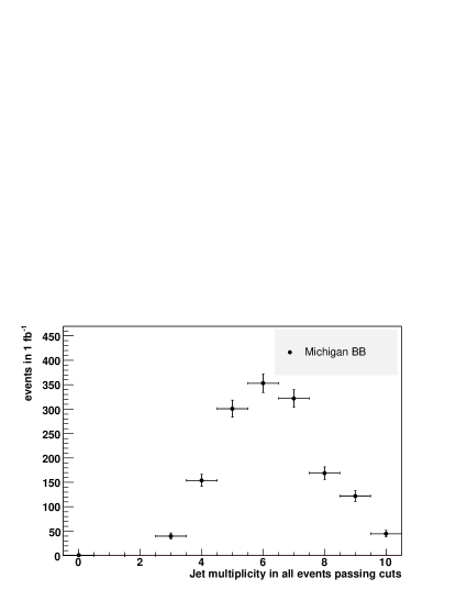
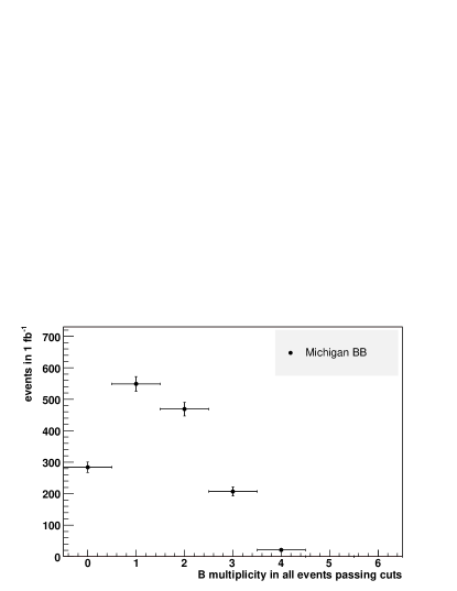

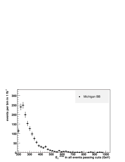

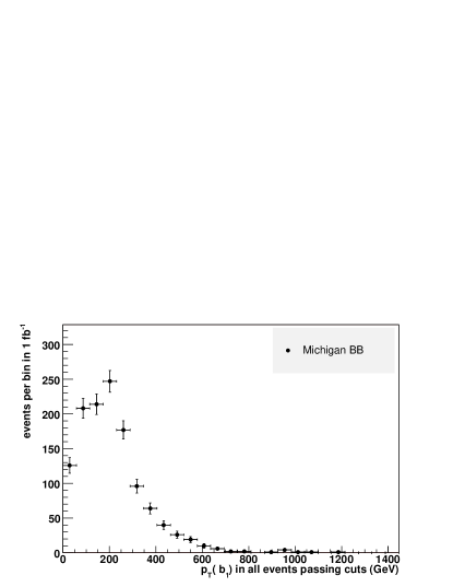
4.2 Building an OSET for the Signal
Signal-only distributions in , , and are shown in Figure 29 below, as are histograms of reconstructed jet and -tagged jet counts (for a cone size ) in Figure 28. These distributions and all that follow are after application of the cuts of Table 2. The signal we have found is dominantly hadronic with appreciable missing energy; high -jet multiplicities suggest that third-generation partners play a special role. We can try to make more precise claims about the partonic final state of the signal events, but must do so with care—multiple processes are involved, and tagging efficiencies are momentum-dependent. We will restrict our attention here to new-physics interpretations with SUSY-like decay topologies, where arises from a pair of stable, neutral decay products. It is also prudent to evaluate the consistency of the observed excess with topologies with no new invisible products, where is the result of jet mis-measurement or comes from neutrinos. Note that our definition of as the sum of ’s of all reconstructed objects and missing energies differs from the definition (here ) used in the CMS Physics TDR and in our cuts.
Let us begin by checking that the OSET we would guess from the correct Lagrangian is indeed successful. We assume the correct spectrum—a new adjoint () a stable neutral particle () to which it decays, and a charged state nearly degenerate with the neutral state (the hypothesis of near-degeneracy could be disproved by the presence of extra hard leptons in the decays). We will focus on the graphs of Figure 30, ignoring the electroweak processes in Figure 31 because of their low trigger rate and high background contamination. A MARMOSET input file for this OSET is shown in Figure 32. For these masses, decays are kinematically forbidden, and we will not include them in our analysis.
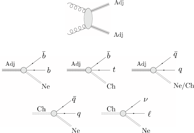
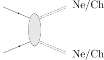
# Standard Model Particles d dbar : pdg=1 charge=-1 color=3 mass=0.33 u ubar : pdg=2 charge=2 color=3 mass=0.33 b bbar : pdg=5 charge=-1 color=3 mass=4.8 t tbar : pdg=6 charge=2 color=3 mass=175.0 g : pdg=21 charge=0 color=8 mass=0 e- e+ : pdg=11 charge=-3 color=0 mass=0.00051 nu_e nu_ebar : pdg=12 charge=0 color=0 mass=0.0 # New Particles Adj : charge=0 color=8 mass=450.0 Ne : pdg=1000022 charge=0 color=0 mass=124.0 Ch Ch~ : charge=3 color=0 mass=130.0 # Decay Modes Adj > b bbar Ne Adj > t bbar Ch~ Adj > u ubar Ne Adj > u dbar Ch~ Ch > u dbar Ne Ch > e+ nu_e Ne # Production Modes g g > Adj Adj : matrix=1 # Invisible Production Modes (not included) # u ubar > Ch Ch~ : matrix=1 # u dbar > Ch Ne : matrix=1
These three decay mode of Adj populate final states differently: and modes produce four -partons in each pair-production event, and hence have more -tagged jets than ; differs from in having more but softer jets, and sometimes producing leptons. A naive fitting procedure can be used to distinguish these modes. We count events in the Black Box signal with reconstructed jets (), of them b-tagged, and leptons () for triples covering the signal region. These bins are further subdivided into bins according to , and we have used divisions at 700, 1200, and 1500 GeV. 10000 Monte Carlo events are also generated for each of the 16 processes in the OSET; these are run through the PGS detector simulator, and events are counted in the same way. A least-squares fit of the detector-simulated count data produces accurate fits to both the cross-section and and branching fractions as shown in Table 3. At the di-jet decay rate is consistent with zero. Comparisons of signal and OSET Monte Carlo are shown in Figure 33. Note that at this level, the well-motivated OSET used here provides a model-independent characterization of the data.
| Process | Fit Rate | Actual Rate |
|---|---|---|
| 43.1 2.9 fb | 28.0 fb | |
| 0.74 0.04 | 0.77 | |
| 0.25 0.03 | 0.22 | |
| 0.01 0.01 | 0.01 | |
| 0.88 0.11 | 0.60 | |
| 0.12 0.11 | 0.40 |


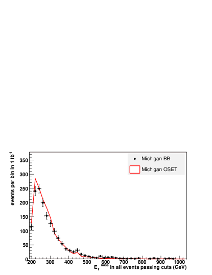

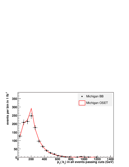
Is this picture consistent with supersymmetry? And if so, what are the SUSY parameters? Two notable aspects of this story are a nearly-degenerate “chargino” (Ch) near the “LSP” (Ne) and the preponderance of 3rd-generation quarks among decay products. Already these facts, readily apparent from the OSET, significantly constrain SUSY explanations—a pure Bino LSP is ruled out, and our attention must be focused on less standard parameter choices. Both properties are accounted for if the LSP is mostly Higgsino, but are also consistent with a Wino or nearly degenerate Wino and Bino—in the latter two cases, the preponderance of 3rd-generation decays could be explained by 3rd-generation squarks much lighter than the other squarks. At this point, we cannot readily distinguish the two scenarios in Figure 34. In either case, study of soft leptons from leptonic decays could constrain the – mass-splitting, shedding light on the electroweak-ino mixing.
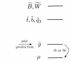
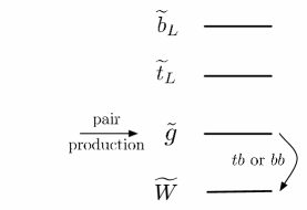
This OSET has served its two purposes well. It suggests regions of theory space consistent with the data. At the same time, it offers a more efficient and transparent characterization of the data than the full model would; the cross-section and branching ratios we have found are determined in the SUSY models not only by the on-shell masses but also by many neutralino-mixing parameters and squark masses. But could we have arrived at it without knowing the model in advance?
4.3 Mass Determination
As is well-known, accurately determining absolute mass scales is difficult in cases where full event reconstruction is not possible. We do not add any new techniques for mass determination here, and only comment on how mass scales can be inferred in an OSET context. We have chosen the masses in this OSET with foresight, but could they have been determined from the data? At low luminosities and with the smearing of jet energies, we cannot easily reconstruct any sharp kinematic features (edges and endpoints at the boundaries of phase space) that permit precise mass measurement. Nonetheless, if the detector response to jets is well-calibrated on Standard Model processes, we can resolve various particle masses from the shapes of distributions.
For example, raising the mass of the particle that is pair-produced significantly affects the kinematics of decays—all products carry more momenta, so that and (shown in Figure 35), as well as individual object ’s, increase correspondingly. A shift of 100 GeV begins to be resolvable.
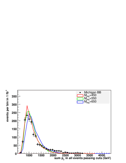
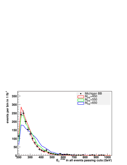
The leading effect of on the available decay phase space can be reduced by increasing the mass of , the stable final-state particle, in lockstep. This shift, illustrated in Figure 36, keeps visible object ’s fixed, but we see that some difference in is still visible.
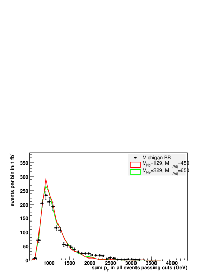
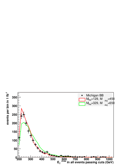
It should be noted that the mass scale determined by these means assuming a flat production matrix element will be inaccurate if a threshold-suppressed contribution to is important. Therefore, it would be important to test the systematic effects of different matrix element choices on mass determination.
One other element that can be used to constrain masses indirectly is the production cross section; within a model with no free couplings, this is determined by particle masses. In some regions of parameter space, the rate depends only on the mass of the particles being produced, while in others, a number of intermediate-state masses and couplings play an important role in determining the production cross section. This is one reason that leaving as a free parameter, as is done in an OSET, is desirable as there are often theoretical uncertainties in assumed mass/rate correlations. Another difficulty in tying production rates to masses is that the predictions differ among different models, so a mass measurement assuming SUSY will be different from the mass measurement assuming a different underlying model. By using an OSET parametrization, these theory systematics can be understood by varying matrix elements in a model-agnostic way.
4.4 False Starts
To achieve confidence in an OSET, it is essential not only to obtain reasonable agreement between the data and OSET predictions, but also to rule out reasonable alternative hypotheses. The ease of generating Monte Carlo for a class of candidate OSETs all at once –accounting for branching ratios by re-weighting events instead of re-simulating them–makes this computationally difficult task far more approachable. The interplay of quick comparisons of OSET-level event generation to data and theoretical inferences is also essential. Here, we will not rule out alternatives thoroughly, nor even to our own satisfaction; we merely seek to outline how an analysis could proceed, and highlight this interplay.
The distributions and counts we have seen and the agreement of the data with the OSET of Section 4.2 suggest production of quarks and ’s; -jet counts are consistent with four ’s per event. We will assume that deviations from this counting are not dramatic. Though the process shown in Figure 37 could produce the desired final state, we reject it for several reasons: it is likely sub-dominant relative to the pair-production process of Figure 30; it must be accompanied (if not dwarfed) by the 2- and 6-quark symmetric decay chains that it implies, producing a larger spread in jet multiplicity; and these decays would be quite asymmetric, with one jet typically much harder than the others.
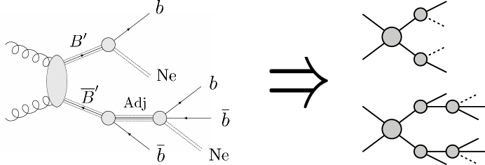
Two more subtle modifications to the OSET of Figure 30 merit further scrutiny. One possibility is that the new triplets assumed to mediate the 3-body decay could be on-shell rather than off-shell; another is that some or all of the ’s could arise from electroweak cascades rather than quarks. An OSET for the first alternative is shown in Figure 38 and Table 4.
The mass of the has been tuned to minimize the difference among transverse distributions used in this analysis. The minimal differences with a tuned mass are illustrated in Figure 39. Given the combinatorial background, it is difficult to resolve a difference between on- and off-shell by using di-jet invariant mass distributions, looking for an edge versus and endpoint. More sophisticated analysis should be employed to resolve these cases. In this case, we resort to somewhat indirect logic: if the is strongly interacting, then it should be minimally produced through QCD.

| OSET Spectrum | |
|---|---|
| 450 GeV | |
| 360 GeV | |
| 128 GeV | |
| 124 GeV | |
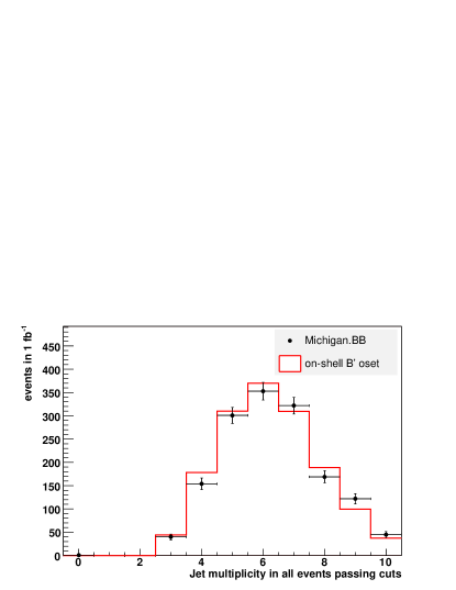
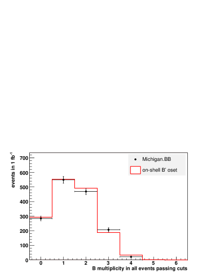
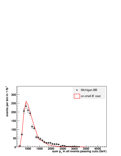
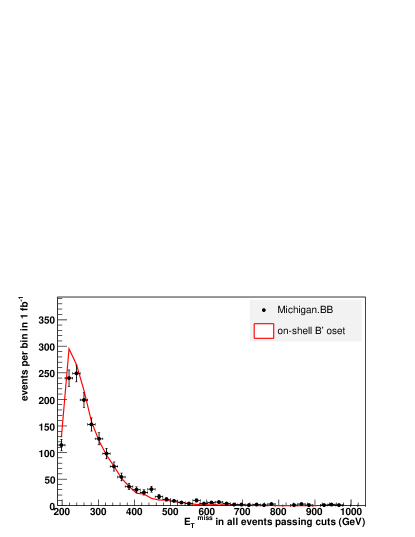

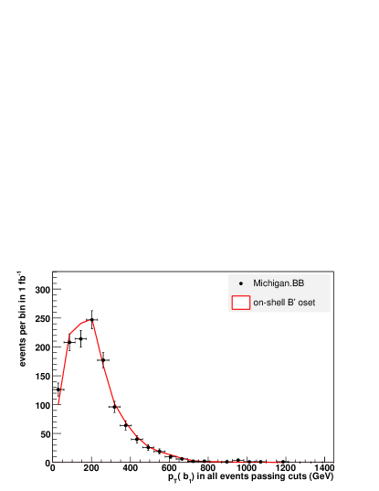
A sbottom search in the channel with a final state (or potentially with a or final state with additional soft charged particles) could be used to constrain the production of this . If results are presented as limits on for this topology, as functions of and , they could be readily interpreted for application to any model or to an OSET analysis. Some mass range will be excluded when one assumes only QCD production, with different exclusions depending on the spin, but the limit is robust. If minimal production can be excluded at the mass for which other distributions do not show a difference, then we can rule out this scenario. Arguments along these lines could help restrict this class of model, with .

| OSET Spectrum | |
|---|---|
| 450 GeV | |
| 300 GeV | |
| 128 GeV | |
| 124 GeV | |
The third possibility (’s arising from electroweak cascades, as in Figure 40) is more interesting: with this choice of mass, no clear differences exist in single-particle momenta, , or distributions, or counts (Figures 42 and 41). So in fact the branching ratio could consist of any combination of (Figure 30) and (Figure 40) as far as this analysis could tell.


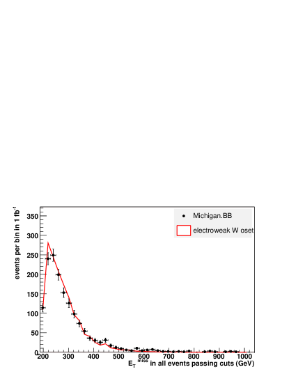

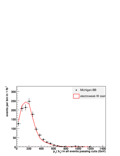
Given this ambiguity, two directions should be explored simultaneously; one is experimental, the other theoretical. With the complicated detector environment, we have made no attempt to explicitly reconstruct tops, but a thoughtful look at more correlated observables could show evidence of top quarks in the decays. One can also look at additional variables to try and discriminate among these event shapes. On the other hand, theoretical considerations suggest other signals to look for: if the decay is present, and and form an doublet, then should also appear with a comparable rate. By searching for leptonically decaying ’s in these events, we can indirectly limit the decay rate of .
4.5 Sub-dominant Process or Poorly Modeled Tail?
The plot for the best-fit OSET has captured the bulk of the signal events, but the overall count with is inconsistent with the OSET at . The actual significance of this excess at the LHC at depends on the Standard Model contribution and its uncertainty, and on the precise cuts used in the analysis. But assuming that it would eventually be identifiable as new physics, we wish to consider its interpretation within this class of possibilities: is it “old” new physics (a poorly modeled tail of the underlying model’s pair-production process) or a new process altogether?
Among new processes, two well-motivated ones deserve particular attention. The three-body decays must be mediated by new color triplets. Assuming flavor isn’t badly broken, these are bottom- and/or top-type ; they can be pair-produced, but associated production with is probably quite suppressed. Approximate flavor universality would again suggest light-quark partners , and these could be produced in association with quarks as in Figure 43.
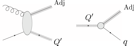
The former possibility can of course be evaluated by comparing the high- data to model Monte Carlo, but the matrix element parameterization of the previous section allows a similar analysis within an OSET. For clarity, we will study this smaller effect in of data. This is not a realistic discovery threshold, but the point at which the differences between the models we consider are apparent, in the absence of backgrounds, through our simple observables.
Figure 44 illustrates the discrepancy between our OSET fit with flat matrix elements and the Black Box “data” signal, as well as the distribution in an OSET where we have attempted to absorb the tail into a more general matrix element. We have added terms (in the parameterization of Section 2.1) to the production matrix element, as these are the terms that fall slowest, even well above threshold. We also examine the high- tails of the improved OSET in more detail in Figure 45. In fact this is not enough—because we know that modifying the matrix element shifts the peaks of distributions (and hence of ) as well as the tail. Therefore, we also search for OSETs that compensate for this effect by lowering .
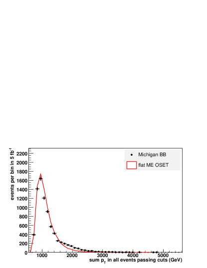

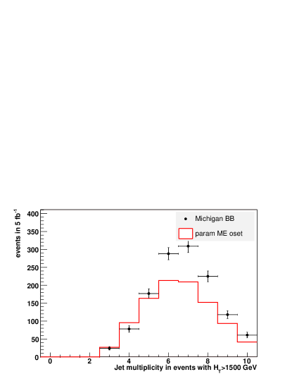
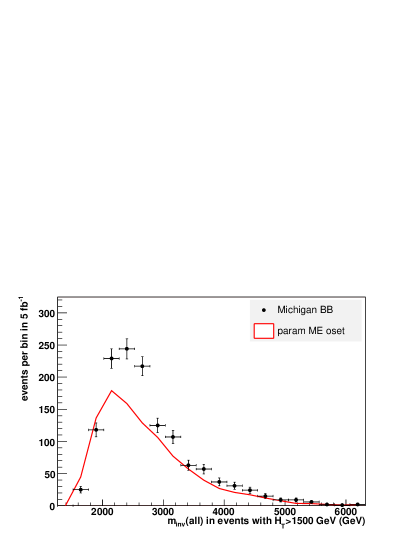
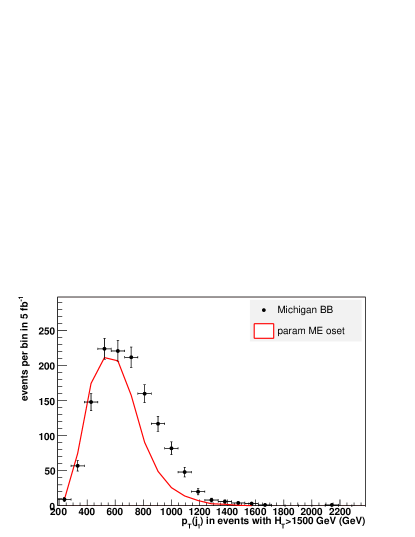
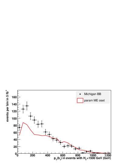
We note a few features of the events on this tail that are not consistent with a matrix element correction: these events have higher jet counts, but comparable -tagged counts to the OSET. The leading jet is harder than in the OSET, while the leading -jet is softer. Such an asymmetry can only come from a new production process. Both of these facts suggest that the events on the tail come from a process that produces an extra light-flavor jet—given our previous theory prejudice, a heavy triplet in associated production with is an excellent guess. We have added the 1870 GeV triplet to the model, which decays to (here is a stand-in for any light-generation quark). The overall distribution for a fit to this OSET is shown in Figure 46. The plots restricted to the high- tail are shown in Figure 47. Comparing Figures 45 and 46, we conclude that the high excess is more consistent with the additional processes suggested in Figure 43 than with a mismodeling of the adjoint pair production matrix element. A final rate fit with the new channel added is given in Table 7.
| OSET Spectrum | |
|---|---|
| 1870 GeV | |
| 450 GeV | |
| 128 GeV | |
| 124 GeV | |
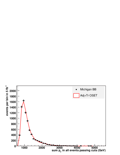
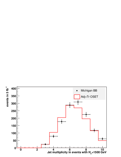
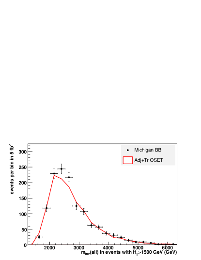
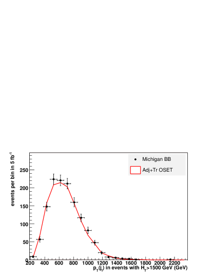
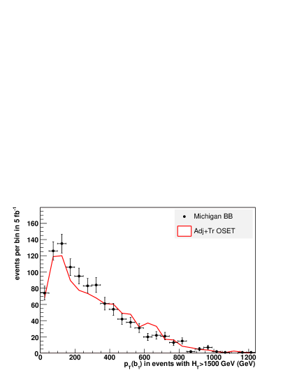
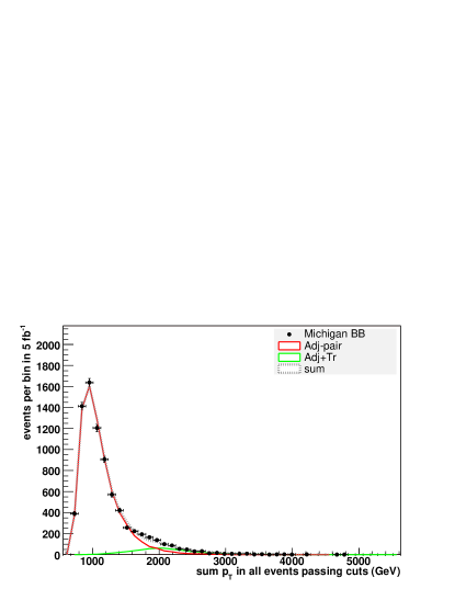
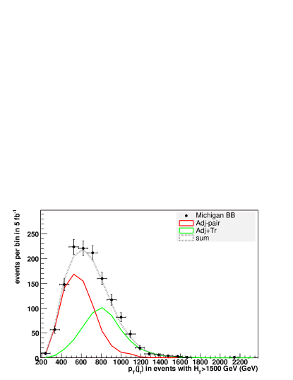
| Process | Fit Rate | Actual Rate |
|---|---|---|
| 30.1 0.9 fb | 28.0 fb | |
| 0.31 0.04 fb | 0.41 fb | |
| 1.0 | 1.0 | |
| 0.82 0.03 | 0.77 | |
| 0.17 0.02 | 0.22 | |
| 0.01 0.01 | 0.01 | |
| 0.56 0.10 | 0.60 | |
| 0.43 0.10 | 0.40 |
4.6 OSETs and Data Characterization
The process of zeroing in on the correct theoretical description of an unexplained signal, whether it arises from new physics or from the Standard Model, will not be easy. No characterization scheme can remove the fundamental difficulties associated with uncertainties in Standard Model implementation, nor the loss of information inherent in hadronic collisions and decays. These questions are hard to answer, but the OSET description has at least facilitated asking them.
The success of simple rate-fitting techniques in this example should be viewed skeptically—the Standard Model background is absent, the detector simulator agrees perfectly with the detector, and systematic errors in this approach are difficult to quantify. The primary benefit of an OSET fit is in rapidly determining key qualitative features of new physics—the types of new particles, their approximate masses, and which decay modes dominate, as represented in Figure 49. The agreement is striking.
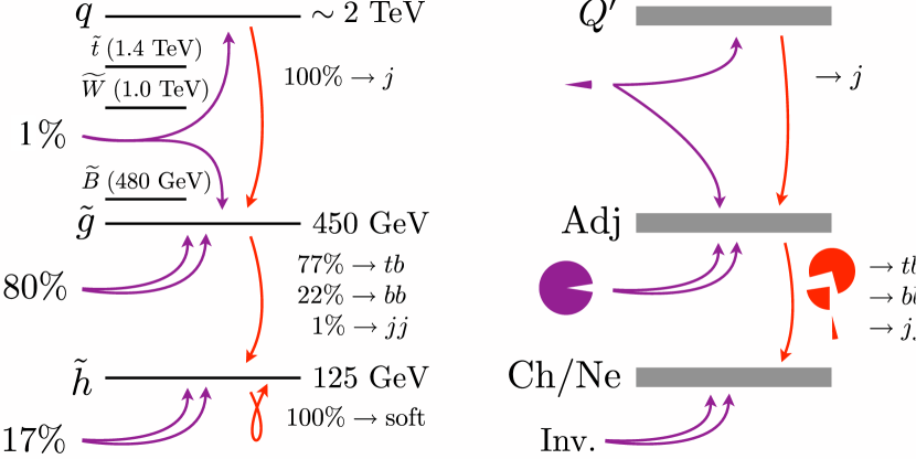
Even the qualitative level of detail of this description is enough to sharply focus our model-building intuition. The first OSET fit has guided us to two possibly consistent MSSM scenarios—a or LSP. The second relies on a mass splitting to explain the hierarchy of branching ratios—disfavored by the presence of a channel highly suggestive of squark-gluino associated production.
5 Concluding Remarks
We have shown that On-Shell Effective Theories are an effective bridge between LHC data and the fundamental theory at the TeV scale, in a wide range of possible scenarios for new physics. This is especially important for theories with a zoo of new particles, complicated production mechanisms, and long decay chains. MARMOSET is a simple Monte Carlo tool for directly simulating OSET descriptions for new physics. An OSET motivated by new physics signals captures important qualitative features of the underlying model of new physics and strongly constrains its structure. The examples in this paper illustrate the productive interplay between physically motivated data characterization and model-building.
The first data from the LHC has the potential to revolutionize our understanding of fundamental physics. The collective effort of experimentalists and theorists should guide us the new Standard Model. A physically meaningful characterization of collider data will play a critical role in making this happen. OSETs and MARMOSET can act as clear conduits of information between experimentalists and theorists in the era of discovery. In the hands of experimentalists, MARMOSET can be used to characterize new physics discoveries and exclusion limits in a transparent way—this sort of information will be invaluable and easily understood by theorists outside the collaborations. In turn, theorists can cast their favorite Lagrangians in terms of an OSET which can be readily compared to data.
An OSET characterization of LHC data is not an end in itself but a waystation on the path to a fundamental theory. The OSET framework will only be successful if it leads to a compelling Lagrangian that obviates the need for an OSET description. Ultimately, understanding the structure of this effective Lagrangian will unveil the new principles of Nature long anticipated at the weak scale.
Acknowledgments
We are indebted to Johan Alwall, Matthew Baumgart, Liam Fitzpatrick, Tom Hartman, Jared Kaplan, and Itay Yavin for furthering the development of MARMOSET through their programming efforts. We thank Rikard Enberg, Paddy Fox, Roni Harnik, Michele Papucci, and John Terning for testing MARMOSET in its infancy.
We benefitted greatly from conversations with Dante Amidei, John Conway, Su Dong, Melissa Franklin, Henry Frisch, Fabiola Gianotti, Eilam Gross, Joao Guimaraes da Costa, Valerie Halyo, Tao Han, Beate Heinemann, John Huth, Gordy Kane, Paul Langacker, Patrick Meade, Michael Peskin, Aaron Pierce, Leonardo Rastelli, Matt Reece, Albert de Roeck, Maria Spriopulu, Matt Strassler, Scott Thomas, Chris Tully, Herman Verlinde, Gordon Watts, and Charlie Young. Discussion of the “Michigan Black Box” draws heavily from the work of all involved in the LHC Olympics, particularly Matt Bowen and Matt Strassler for their inspiring first assault on the problem, the members of the Harvard Michigan Black Box team, and the creator of the black box, Gordy Kane. Special thanks to the entire LHCO community for stimulating and facilitating the development and study of numerous data challenges.
The work of N.A.-H. is supported by the DOE under contract DE-FG02-91ER40654. P.S. and N.T. are each supported by National Defence Science and Engineering Fellowships. J.T. is supported by a fellowship from the Miller Institute for Basic Research in Science. The work of L.-T.W. is supported by the National Science Foundation under Grant No. 0243680 and the Department of Energy under grant DE-FG02-90ER40542. Any opinions, findings, and conclusions or recommendations expressed in this material are those of the author(s) and do not necessarily reflect the views of the National Science Foundation. S.M. is supported by Fermi Research Alliance, LLC under Contract No. DE-AC02-07CH11359 with the United States Department of Energy.
Appendix A Structure of Non-Resonant Scattering
In this appendix, we address the physics of production processes. The main point of an OSET parametrization scheme is to capture the possible kinematic shapes of variables that are useful for untangling and interpreting new physics. For now, we will focus on inclusive single object rapidity and distributions. As we’ll see and as the reader might find intuitive, we can tremendously improve our scheme over the constant approximation by including the leading order near-threshold behavior of matrix elements. Less intuitive and more useful to exploit is that for rapidity and variables, there is a large shape degeneracy among the possible matrix element behaviors. When we exploit these shape degeneracies, we will find a simple parametrization scheme that captures both rapidity and shapes. Empirical results appear in Appendix A.2 which are more fully justified in Appendix A.3.
A.1 Parametrizing Particle Production
Let’s start by introducing some notation and basic formulas to facilitate our analysis. For a general process (we assume and are massless), the kinematics can be completely described in terms of the familiar Mandelstam variables , , and , where are the four-vectors for particles , , , and . If we are working in the center-of-mass frame, it is convenient to express both and in terms of and as,
| (17) |
where is the center-of-mass scattering angle, are the final state masses, and
| (18) |
In the lab frame, it is convenient to express the final state kinematics in term of the transverse momentum squared
| (19) |
as well as the rapidity of one of the final states (say particle ):
| (20) |
where are evaluated in the lab frame. As is well known, rapidity is additive under longitudinal boosts, so it is often easier to work in terms of the center of mass rapidity and then boost by the initial state rapidity to get back to the lab frame.
In what follows, we will be interested in computing differential distributions for the transverse momentum as well as the rapidity . Following the usual parton model for hadronic collisions, we start with the full differential cross section
| (21) |
where the are the parton distribution functions, is the momentum transfer squared of the process, are the longitudinal momentum fractions of incoming particle and respectively, , and . The squared matrix element for any process is proportional to the differential cross section for scattering, , hence we’ve isolated this piece in Eq. (21).
For convenience, we adopt a set of dimensionless variables with which to express our results. For the process , let’s define dimensionless and variables as
| (22) |
where is the threshold center-of-mass energy squared. We also introduce final state mass asymmetry parameters and as
| (23) |
so that as . In terms of our dimensionless variables, we can express the kinematic quantities and :
| (24) |
The lower boundary of phase space occurs when , and the upper boundary depends on the beam center-of-mass energy squared , yielding
| (25) |
Note that . The longitudinal momentum fractions can be expressed as
| (26) |
and we see that the initial state rapidity is constrained between , where
| (27) |
Before calculating differential distributions, it is convenient to define dimensionless “parton luminosity” functions
| (28) |
Figure 50 displays the integrated “parton luminosities” for several different initial states at . For simplicity, the logarithmic running of the PDFs as a function is ignored in performing this integration.
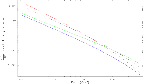
As can be seen, for a given value of , it is often a very good approximation to take , valid over a region from to . Typical values of fall in the range of . Many of the properties of that we will discuss later will follow from this simple parametrization. Another useful fact that we will exploit is that the parton distribution function can be parametrized as
| (29) |
where and . We will ignore , as it is often negligible and will not effect our basic results in later subsections. For understanding , we will use the fact that is well-behaved in .
Throughout the remainder of our discussion, we will ignore the logarithmic running of the with and the running of any couplings. Having made that approximation, which is valid to the level for most of the quantities we will compute, we can express the full differential cross sections in dimensionless form. Taking either , , or as independent variables, we can rewrite Eq. (21) as
Ultimately, we are interested in differential distributions for and . We can integrate Eq. (A.1) to calculate and as
| (31) | |||||
| (32) |
In the next subsections, we explore the shapes of and for different values of .
A.2 Rules of Thumb
Perhaps the simplest way to parametrize scattering is to approximate the behavior of the matrix element as the sum of rational polynomials in and ,
| (33) |
As an empirical exercise, we can compare the and distributions for matrix element of the form . This is illustrated in Figure 51 for distributions.
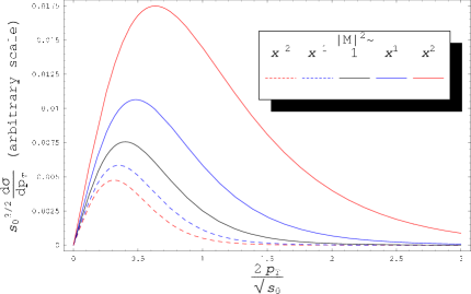
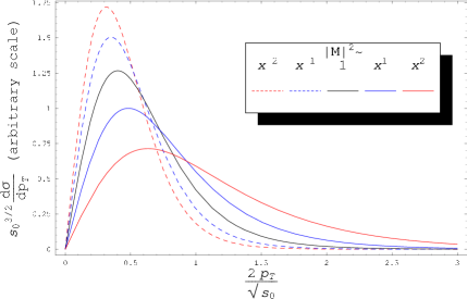
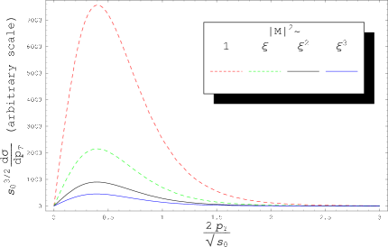
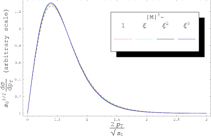
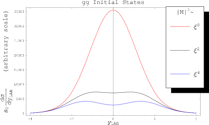
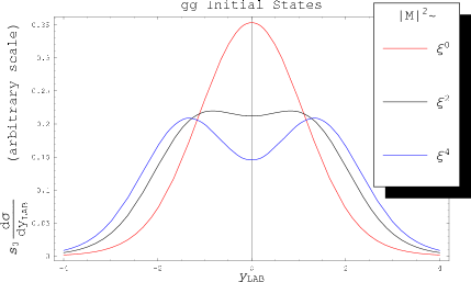
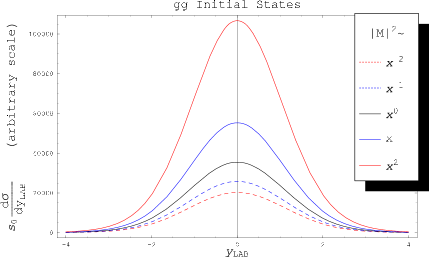
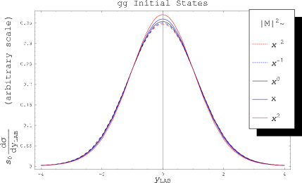
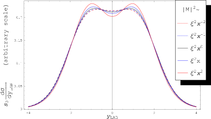
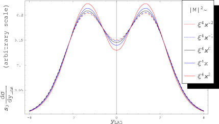
As is clearly evident and hardly surprising, for the moments of the distributions increase/decrease with increasing/decreasing powers . More surprising is that the shapes of the distributions do not depend on ! Illustrated in Figure 52 are the rapidity distributions for varying choices of . Evident is the strong correlation in the shape structure of the rapidity distribution with while there is essentially no dependence on .
Equipped with these observations, we are ready to state some generally applicable and very useful results for modeling and observables. We argue that for general non-resonant processes:
-
•
The shape of is well-parametrized by leading order in behavior without regard to dependence. This works because of an approximate shape invariance of under . In most cases, including only leading order behavior suffices to capture the transverse structure at the level.
-
•
An approximate shape invariance of under allows one to model the structure without effecting the shape modeling of .
-
•
Once the transverse structure is well modeled, the rapidity structure is usually fixed by the PDF structure with sub-leading correction in . Moreover, inclusion of these sub-leading corrections does not effect the distributions by virtue of the shape invariance of .
We will rigorously demonstrate these points below. As these results will help define our leading order OSET parametrization scheme for particle production, we will also identify where and why the above properties fail. The application of these results to the modeling of full decay topologies is the topic of Secs. 2 and 4.
A.3 Shape Invariance for Transverse and Rapidity Structure
Let’s first understand the shape invariance of under . We’ll start by returning to Eq. (31) and write
| (34) |
Expanding a general matrix element as
| (35) |
and taking advantage of the property illustrated in Figure 50 that the the integrated “parton luminosity” , we have
| (36) |
It is straightforward to evaluate this expression analytically order by order in an expansion in the mass asymmetry parameter . We will drop small logarithmic corrections arising from Altarelli-Parisi running. Expanding to first order in ,
| (37) | |||||
where we have defined and taken , a good approximation given that the integrand is dominated away from (recall that for any reasonably behaved matrix element and PDF). Evaluating these integrals,
| (38) |
where is the Euler Beta function.
From Eq. (38), it’s clear that the shape invariance is the result of the approximate homogeneity in of both the parton luminosity functions and . Of course, there are corrections that are not shape invariant, but these are suppressed not only by , but by and Euler Beta function factors with respect to the leading order behavior. An illustration of the shape deformation in the partonic distribution is shown in Figure 53 with (which corresponds to ). Another important fact can be read off from Eq. (38), namely the Euler Beta suppression with decreasing powers of explains why the leading order behavior is usually sufficient to capture the shape.

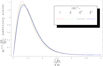
The above observations make it clear that the leading order transverse structure is controlled by the leading order dependence of . We also see that this should start to fail in cases where the final state mass asymmetry is large (i.e. ), in which case small shape corrections may be needed. For small , note that we can actually get away with choosing the wrong PDFs as long as we compensate for the transverse shape by also choosing the wrong dependence of the matrix element. If one is interested in extracting the correct dependence, then we will see that rapidity information can be used to constrain the PDFs.
We turn now to understanding the approximate shape invariance of under . Let’s start with Eq. (32) and write,
| (39) | |||||
where
| (40) |
and we’ve used the expansion in Eq. (35), Eq. (A.1), and defined a small expansion parameter that controls the available initial rapidity phase space. We’re also taking advantage of the fact that only depends on .
From Eq. (29), we see that has a pole in near . Factoring out the pole, the integrand of has a well-behaved polynomial form if we expand in . But and in only appears in the combination , so we know that at leading order in , the and dependence of the integrand must factorize. After doing the integral, we are guaranteed to find
| (41) |
where is a function of , , and alone. The PDF information is largely contained in . To see why the corrections occur at instead of , recall that the boundaries of phase space are given by , so the integral over spoils the factorization before the higher order corrections from .
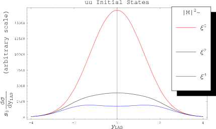
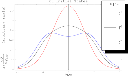
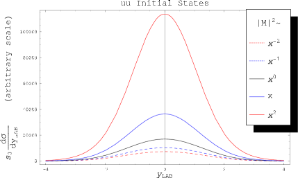
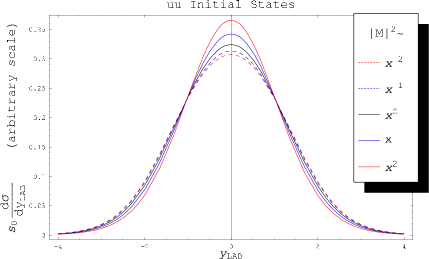
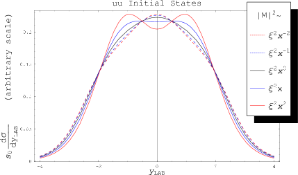
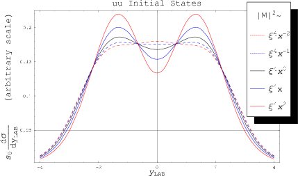
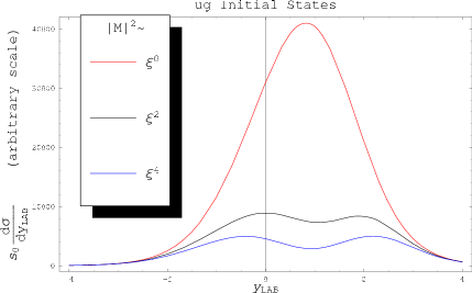
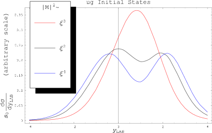
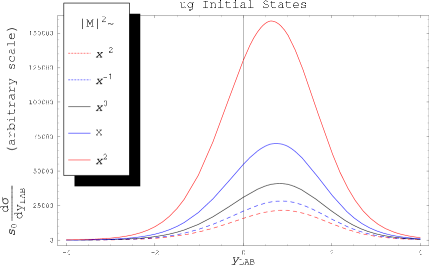
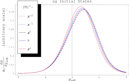
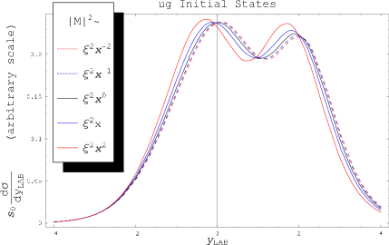
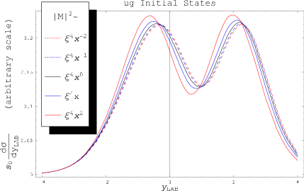
With this result, Eq. (39) takes the form
| (42) |
From this, we see that at leading order in , the integral over does not affect the dependence of ! Consequently, we expect only the normalization of to change at leading order under . We also see that the leading order rapidity shape structure is controlled by the PDFs quite explicitly!
The above argument tells us that the success of factorization depends on whether or not we explore phase space boundaries. For with non-zero , the matrix element favors large rapidity so the -dependent boundary is more pronounced, leading to largish violations of shape invariance. Figures 54 and 55 show rapidity shapes and variations for different choices of behavior. The rapidity shape invariance under turns out to be numerically less accurate than the transverse shape invariance under , but because the rapidity distributions are controlled mostly by PDFs anyway, getting a robust matrix element parametrization is less important than choosing the right initial state partons.
Appendix B A Useful Parametrization With Examples
In Appendix A, we argued that once PDFs are folded into partonic matrix elements, there exists useful shape invariance relations. These shape invariances allow us to capture the leading LHC signatures through a small set of basis matrix elements.
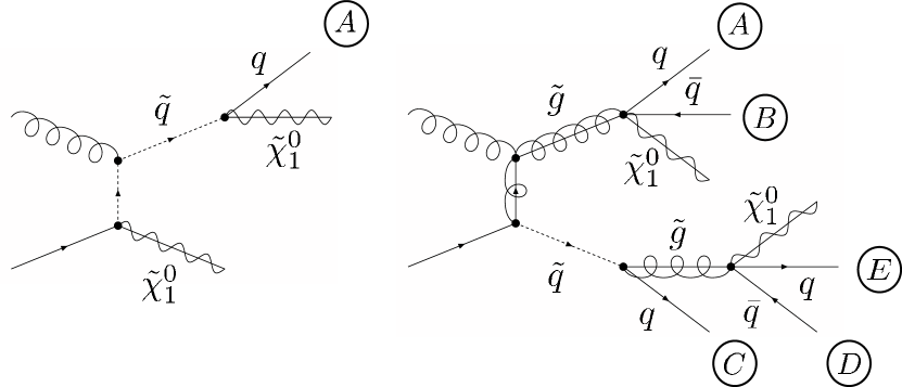
| Particle | Mass (GeV) |
|---|---|
| 1106 | |
| 2000 | |
| 199 |
Here, we give several concrete examples where the matrix element parametrization of Section 2 is indeed effective. In Appendix B.1 we give two examples where a two-parameter matrix element fit is sufficient to accurately reproduce almost all final state kinematic distributions. In Appendix B.2, we show how spin information is washed out both by PDF integration and cascade decays. While we have made no attempt to justify the OSET parametrization in every conceivable topology, the examples in this appendix provide ample anecdotal evidence to warrant a more complete study within the context of a realistic detector simulation. All examples are either based on the topologies from Figure 13 or on new topologies defined in Figure 56.
Indeed, for an experimental collaboration, these kinds of case studies can be used to optimize the discovery potential for particular topologies, regardless of the dynamics of the underlying physical model. It may be easier to search for certain pathological matrix elements that violate the shape invariance relations we found, or the persistence of shape invariance might influence the types of experimental cuts used in general searches. Once a discovery is made, the shape of kinematic distributions may provide hints as to the underlying model, so it will be important to know which distributions are most sensitive to detailed dynamics. In the plots that follow, we look only at single object observables; undoubtedly, there exist correlated observables that can be analyzed at high luminosity for which higher order correction must be included in the OSET parametrization scheme.
B.1 Two-Parameter Fits
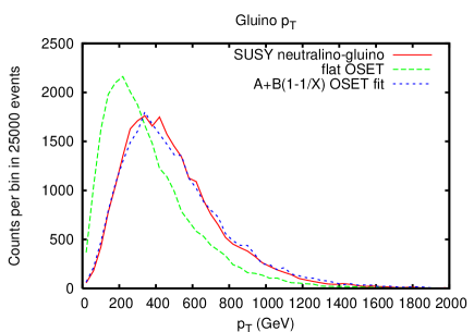

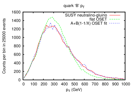
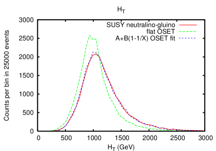
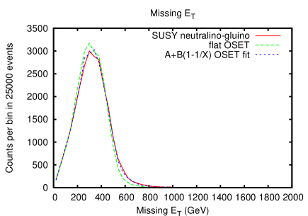
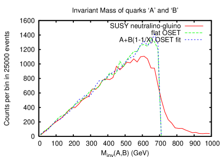
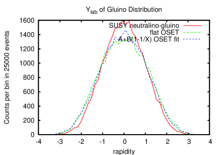
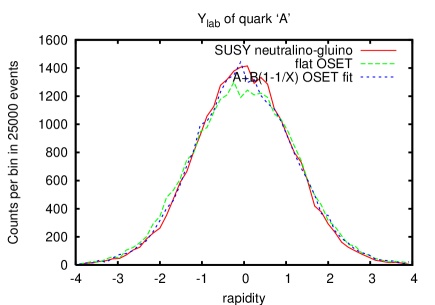
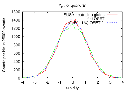
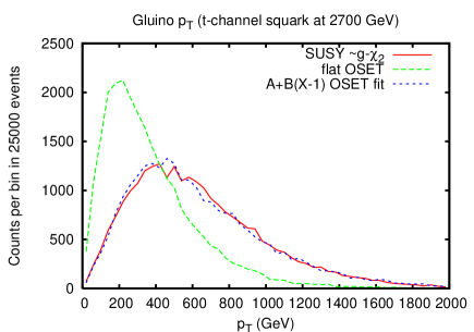

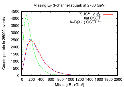
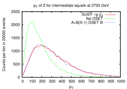
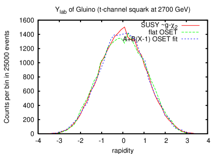
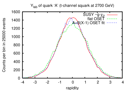
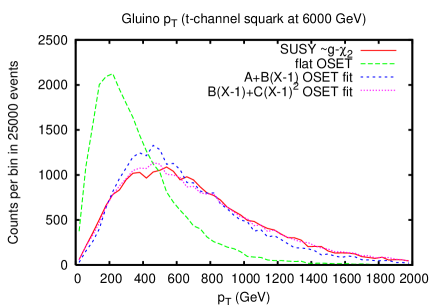
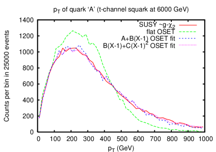
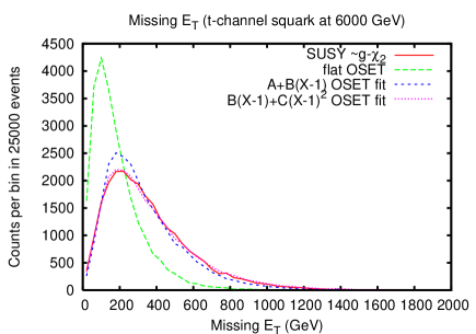
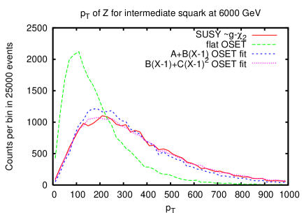
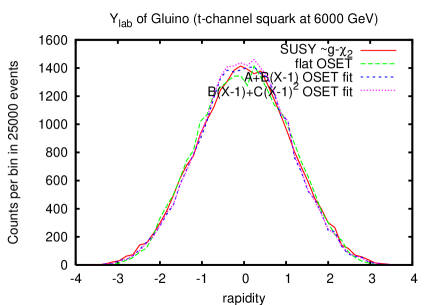
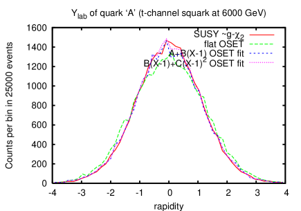
The first example (Figures 57 and 58) comes from the SUSY associated production channel from Figure 13. Despite the fact that this process exhibits -wave suppression, there are pieces of the amplitude proportional to powers of , so the transverse shape invariance of means that there is an effective contribution to the amplitude. As shown in Figures 57 and 58, a constant amplitude gives a reasonable characterization of most kinematic quantities. To better model, say, the distribution, we can account for the p-wave suppression of near-threshold events by adding an additional piece. With a leading order shape parametrization (LOSP) of , all single object observables are well-described.
This process has qualitatively different behavior if the -channel (squark) mass is much larger than the threshold value of —in this case, for , grows with like a contact interaction; because of shape-invariance, this is well modeled by a LOSP that grows as a quadratic polynomial in : or . We illustrate this behavior and the success of these fits in Figures 59 and 60. In both cases, the constant term in is negligible; in the former, linear growth describes well, while in the latter including a quadratic term improves the fit.
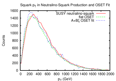
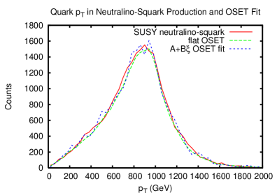
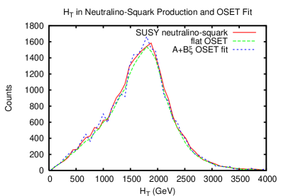
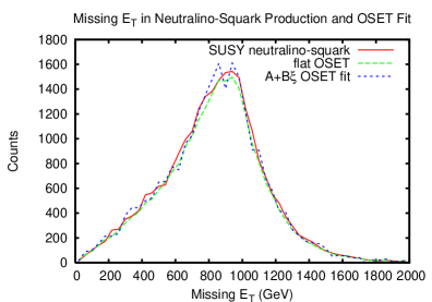
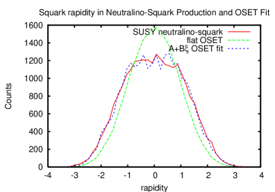
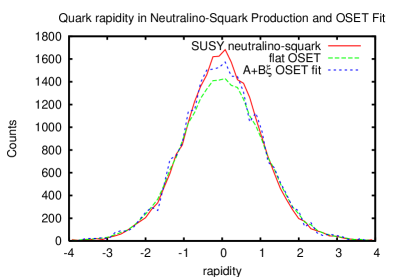
The second example is SUSY associated production from Figure 56. This diagram has a strong -channel pole, and despite the fact that this pole is regulated by the squark mass, we expect the amplitude to contain high powers of . Because of the transverse shape invariance, though, we can capture the distributions in Figure 61 using just a flat matrix element! This indicates the success of transverse/rapidity factorization in matrix element modeling. At leading order, the dependence affects the squark rapidity distribution in Figure 62, but after the squark decays, we see that the rapidity of the resulting jet is more-or-less consistent with the flat ansatz, though a LOSP of does give a better fit.
B.2 Washout of Spin Correlations
In Section 2.2, we saw that in cascade decays, di-object invariant mass distributions can retain information about the spin structure of the underlying model. As is well known, at Lepton Colliders one can use production information to also glean information about spin, but at Hadron Colliders spin information in production is often lost. Here, we show two examples comparing SUSY, UED, and flat matrix elements to see how PDFs and subsequent two-body decays wash out production spin information.
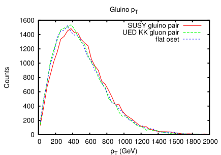

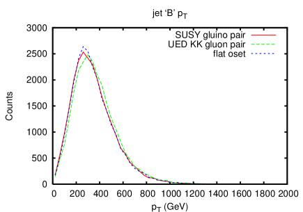
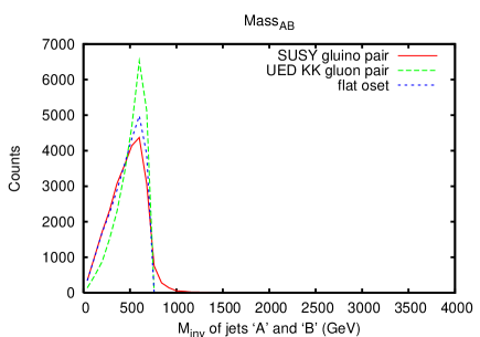
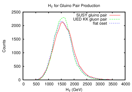
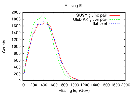
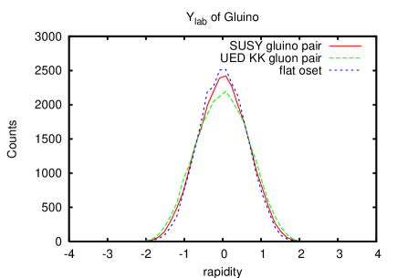
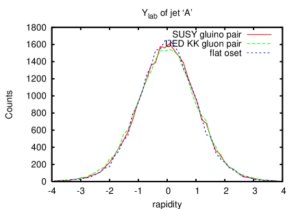

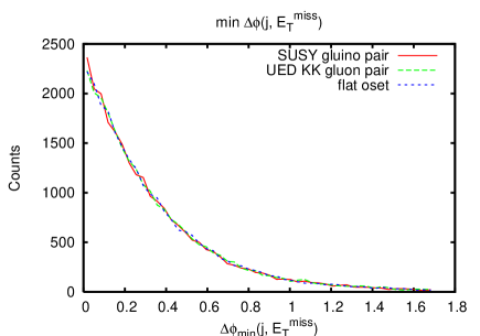
The first example involves color adjoint pair production, i.e. gluino pair production or KK-gluon pair production as in Figure 13. Here, we make no attempt to model the matrix elements beyond a flat ansatz, because both gluino and KK-gluon production have strong pieces which are well modeled in Figures 63 and 64. We observe that while the near threshold behavior of the gluino is more suppressed than the KK-gluon due to a contribution to the gluino amplitude, the effect is small. As expected from Section 2.2, the biggest difference is in the distribution, which measures spin correlations from gluino decays through on-shell squarks, as discussed further in Appendix C. (The extreme sharpness of the KK-gluon edge is due to our not properly taking into account the KK-gluon width. The difference in the shape of the approach is real.) Also noticeable is the small decrease in missing energy in the UED case, due to non-negligible final state correlations.
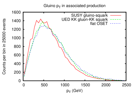
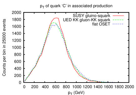
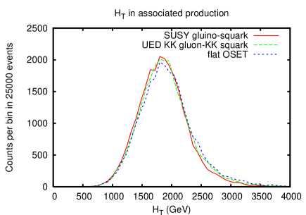
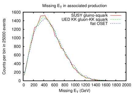
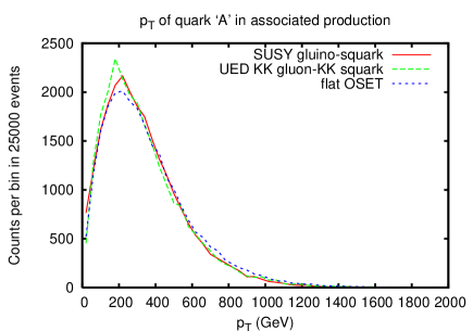
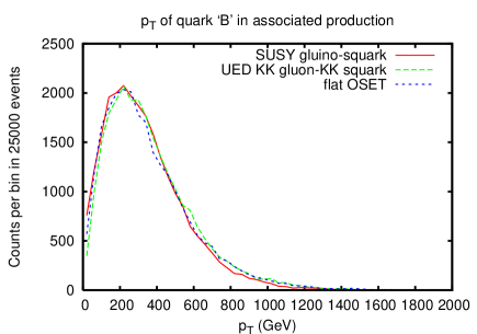
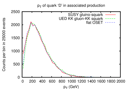
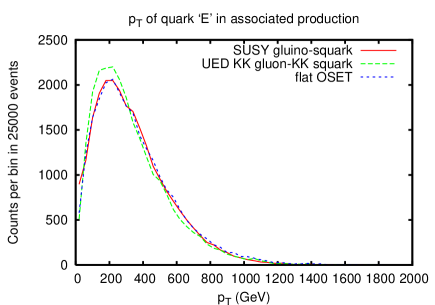
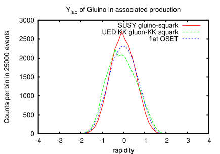
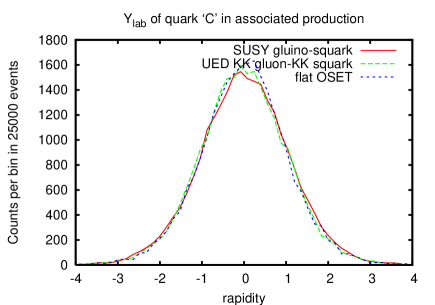
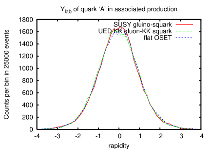
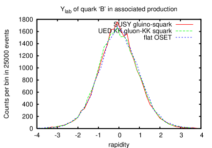
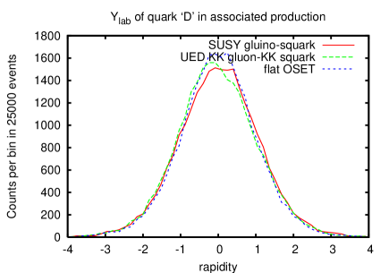
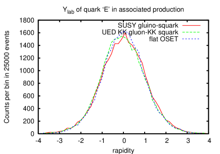
Finally, we look at gluino/squark vs. KK-gluon/KK-quark associated production from Figure 56. In Figure 65, we see a difference in the squark threshold behavior, but it is washed out in the distribution in the resulting quark from the the squark decay. There is little if anything to distinquish SUSY, UED, and a flat ansatz in single particle kinematic distributions in Figures 66 and 67. After the long cascade decays, all distributions are dominated by phase space considerations alone.
Appendix C Spin Correlations and Decay Kinematics: Examples
In this appendix, we develop the discussion in Section 2.2 on the inclusion of spin correlations and the resulting impact on final state kinematics. This discussion is only meant to highlight the basic physics. A more detailed study of this topic is presented in [56].
We have argued that for variables such as and , our approximation captures the leading features. In the rest frame of the decaying particle, there are correlations between the various decay products and the direction of the polarization of the decaying particle. In many cases however, we do not have enough information to reconstruct the rest frame of the decaying particle. Moreover, the directional information is always projected onto the transverse plane of the decay. Therefore, such correlations will tend to be washed out after boosting to the lab frame, which depends on the transverse velocity.
A good example of such an effect is top quark decay. Consider a top quark with some definite helicity. In the rest frame of the top quark, there is a correlation between the direction of the decay products, such as the charge lepton, and the direction of top polarization. On the other hand, if we can only measure the transverse momentum of the lepton, the only effect is that the of the lepton will be somewhat harder (softer) if the top quark is right-handed (left-handed) polarized. On the other hand, this is purely an effect of transverse boost from the top rest frame to the lab frame. If the top quark if produced far away from threshold, such as decaying from a heavy resonance [45], this effect can be significant and carries useful information.
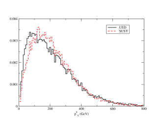 |
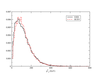 |
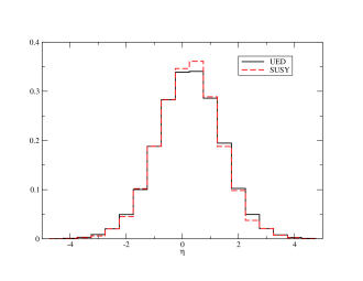 |
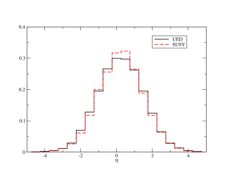 |
On a case by case basis, the origin of such correlation effects is subtle as it depends on the spin of the particles as well as the chirality of their couplings. For most new physics scenarios that we have in mind at the LHC, new particles are mostly produced close to threshold. Therefore, without an extreme boost, we do not expect the spectrum to be severely distorted in our approximation. Similarly, we expect our approximation will be accurate for variables as well. As an example of such a comparison, we compared the jet- distribution in the decay chain . We have used two choices of mass parameters. For supersymmetry, we have chosen the gluino mass to be 700 (400) GeV, the sbottom mass to be 900 (500) GeV, and the LSP (Bino) mass to be 100 GeV. All the other superpartners are decoupled. For comparison, we adopted an UED-like scenario where KK-gluon, KK-bottom, and KK- have the same masses as gluino, sbottom and Bino, respectively. The result is shown in Figure 68. The difference between the two scenarios are not significant. A comparison the rapidity distribution is shown in Figure 69. Although we have presented studies here on the off-shell 3-body decay, we have checked that on-shell decay does not make a qualitative difference to our conclusion (see, for example, Figures 63 and 64).
Another important two object correlation variable is , which is important for isolation cuts. We have compared this variable in the example described above with the same parameter choice, shown in Figure 70. We see that there are virtually no important differences.
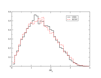 |
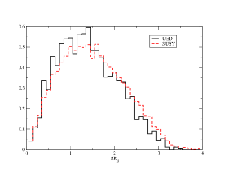 |
We end our discussion on transverse variables with a study of observables that correlate the direction of missing energy and the of any jet. Such variables, , are used to remove QCD background from searches for new physics in hadronic channels. At the partonic level, these distributions are virtually identical for SUSY, UED, and the OSET processes with the same topologies (see Figure 71, again for the and production process).
tbp]
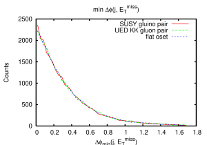
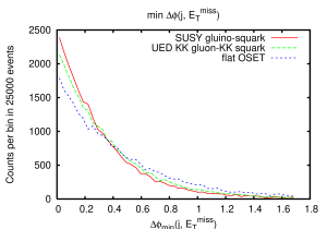
We emphasize here that the difference caused by spin correlations are generally sub-dominant to phase space considerations. The detailed magnitude and structure of the difference will depend on parameter choices and couplings. What we have shown are by no means the best or worst possible cases. More studies are necessary to fully assess the range of possible variations.
Next, we consider invariant mass distributions. To this end, we again consider the decay chain in Figure 18. As we have pointed out in the text, the shape depends on spin identities of new physics particles in the decay chain, the chirality of the couplings and the mass hierarchy.
As an example, we consider the case when is a fermion and both the and couples are left-handed (or right-handed). In this case, the invariant mass distribution has the following form
| (43) |
where depends on the spins of the external particles. When both and are spin-1 vectors (transversely polarized), the slope is positive. On the other hand, if one of them is a scalar, the slope is negative. This fact can be simply understood. In the rest frame of the intermediate particle , the preference of colinearity or anti-colinearity of and is fixed by angular momentum conservation.
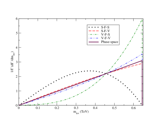 |
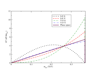 |
Moreover, also depends on the mass hierarchy of the particles involved in the decay chain. For example, in the case that and are spin-1 vectors, the slope will become negative once . In this case, decaying into will be longitudinally dominated and more similar to decaying into a scalar. Such ambiguities in interpretation of the shapes demonstrate perfectly the fact the we must have some information about the mass hierarchy before we can definitely determine the spin of new physics particles.
Therefore, the shape of the two-body invariant mass distributions could vary significantly as a result of the spin correlations. Of course, realistically, we do not expect all two-body invariant mass distributions to carry such clean information, as we are clearly limited by statistics, resolution, and trigger/cuts effects to measure the shape of distributions. Moreover, it is difficult to identify unambiguously the correct objects to pair, in particular if such a combination involve jet object(s). Such combinatorics tends to reduce the statistical significance of any feature in the invariant mass distribution.
Next, we consider the case when the intermediate particle is off-shell and therefore the decay is 3-body. We expect that the effects of virtual particle exchange will be enhanced if it is close to on-shell. Interference between several processes will also be important here. Consider the process in Figure 20. If process dominates, we have a propagator , where . The presence of such an propagator generically pushes the distribution towards smaller . On the other hand, if process dominates, the presence of propagator will push the distribution to higher . Such effects are well-known in electroweak-ino decays when both and the slepton are off-shell [21, 24]. In principle, such deformations could be parameterized by a polynomial of . Given the uncertainties of the shape measurements, we do not expect that we need many terms in this expansion to produce a good fit.
Spin correlation will have an important effect here as well. For example, consider the case where process dominates. If and are fermions and is a scalar, we have no spin correlation between 1 and 2. The propagator forces the distribution to peak at the lower end. On the other hand, consider the case where is a fermion and and are transeversely polarized spin-1 vectors, which has identical couplings as the on-shell example discussed above. A completely parallel argument of angular momentum conservation tell us the distribution is forced to peak more towards the higher . Several examples of such effects are shown in Figure 73.
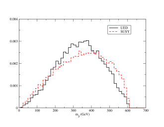 |
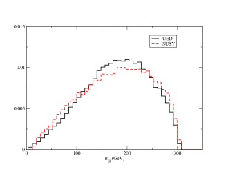 |
References
- [1] UA1 Collaboration, G. Arnison et al., Experimental observation of isolated large transverse energy electrons with associated missing energy at s**(1/2) = 540-gev, Phys. Lett. B122 (1983) 103–116.
- [2] UA2 Collaboration, M. Banner et al., Observation of single isolated electrons of high transverse momentum in events with missing transverse energy at the cern anti-p p collider, Phys. Lett. B122 (1983) 476–485.
- [3] UA1 Collaboration, G. Arnison et al., Experimental observation of lepton pairs of invariant mass around 95-gev/c**2 at the cern sps collider, Phys. Lett. B126 (1983) 398–410.
- [4] UA2 Collaboration, P. Bagnaia et al., Evidence for z0 to e+ e- at the cern anti-p p collider, Phys. Lett. B129 (1983) 130–140.
- [5] CDF Collaboration, F. Abe et al., Observation of top quark production in collisions, Phys. Rev. Lett. 74 (1995) 2626–2631, [hep-ex/9503002].
- [6] D0 Collaboration, S. Abachi et al., Observation of the top quark, Phys. Rev. Lett. 74 (1995) 2632–2637, [hep-ex/9503003].
- [7] D. Green, An lhc run plan: The first inverse femtobarn, hep-ph/0601038.
- [8] Atlas: Detector and physics performance technical design report. volume 1, . CERN-LHCC-99-14.
- [9] Atlas detector and physics performance. technical design report. vol. 2, . CERN-LHCC-99-15.
- [10] Cms techinical design report v.1., . CERN-LHCC-2006-001.
- [11] Cms techinical design report v.2., . CERN-LHCC-2006-021.
- [12] LEP Working Group for Higgs boson searches Collaboration, R. Barate et al., Search for the standard model higgs boson at lep, Phys. Lett. B565 (2003) 61–75, [hep-ex/0306033].
- [13] Higgs Working Group Collaboration, M. Carena et al., Report of the tevatron higgs working group, hep-ph/0010338.
- [14] D0 Collaboration, A. Melnitchouk, Search for non-sm light higgs boson in the h to gamma gamma channel at d0 in run ii, Int. J. Mod. Phys. A20 (2005) 3305–3307, [hep-ex/0501067].
- [15] CDF Collaboration, A. Abulencia et al., Search for new high mass particles decaying to lepton pairs in collisions at tev, Phys. Rev. Lett. 95 (2005) 252001, [hep-ex/0507104].
- [16] D0 Collaboration, V. M. Abazov et al., Search for a heavy resonance decaying into a z + jet final state in p anti-p collisions at s**(1/2) = 1.96-tev using the d0 detector, Phys. Rev. D74 (2006) 011104, [hep-ex/0606018].
- [17] D0 Collaboration, V. M. Abazov et al., Search for associated higgs boson production w h to w w w* to l+- nu l’+- nu’ + x in p anti-p collisions at s**(1/2) = 1.96-tev, Phys. Rev. Lett. 97 (2006) 151804, [hep-ex/0607032].
- [18] CDF Collaboration, Cdf exotics group, http://www-cdf.fnal.gov/physics/exotic/exotic.html.
- [19] D0 Collaboration, D0 new phenomena results, http://www-d0.fnal.gov/Run2Physics/WWW/results/np.htm.
- [20] B. C. Allanach et al., The snowmass points and slopes: Benchmarks for susy searches, hep-ph/0202233.
- [21] H. Baer, C.-h. Chen, F. Paige, and X. Tata, Signals for minimal supergravity at the cern large hadron collider ii: Multilepton channels, Phys. Rev. D53 (1996) 6241–6264, [hep-ph/9512383].
- [22] H. Baer, C.-h. Chen, F. Paige, and X. Tata, Signals for minimal supergravity at the cern large hadron collider: Multi - jet plus missing energy channel, Phys. Rev. D52 (1995) 2746–2759, [hep-ph/9503271].
- [23] S. Mrenna, G. L. Kane, G. D. Kribs, and J. D. Wells, Possible signals of constrained minimal supersymmetry at a high luminosity fermilab tevatron collider, Phys. Rev. D53 (1996) 1168–1180, [hep-ph/9505245].
- [24] I. Hinchliffe, F. E. Paige, M. D. Shapiro, J. Soderqvist, and W. Yao, Precision susy measurements at lhc, Phys. Rev. D55 (1997) 5520–5540, [hep-ph/9610544].
- [25] T. Sjostrand, S. Mrenna, and P. Skands, Pythia 6.4 physics and manual, JHEP 05 (2006) 026, [hep-ph/0603175].
- [26] CDF Collaboration, J. Freeman, Cdf measurement of the top quark mass in the lepton + jets channel using the multivariate template method, Int. J. Mod. Phys. A20 (2005) 3206.
- [27] B. Knuteson, Systematic analysis of frontier energy collider data, hep-ex/0504041.
- [28] B. Knuteson and S. Mrenna, Bard: Interpreting new frontier energy collider physics, hep-ph/0602101.
- [29] 3rd lhc olympics workshop, http://online.kitp.ucsb.edu/online/lhco_c06/.
- [30] P. Meade and M. Reece, Bridge: Branching ratio inquiry/decay generated events, hep-ph/0703031.
- [31] A. Pukhov et al., Comphep: A package for evaluation of feynman diagrams and integration over multi-particle phase space. user’s manual for version 33, hep-ph/9908288.
- [32] A. Pukhov, Calchep 3.2: Mssm, structure functions, event generation, batchs, and generation of matrix elements for other packages, hep-ph/0412191.
- [33] MINAMI-TATEYA group Collaboration, T. Ishikawa et al., Grace manual: Automatic generation of tree amplitudes in standard models: Version 1.0, . KEK-92-19.
- [34] G. Corcella et al., Herwig 6.5 release note, hep-ph/0210213.
- [35] F. Maltoni and T. Stelzer, Madevent: Automatic event generation with madgraph, JHEP 02 (2003) 027, [hep-ph/0208156].
- [36] M. E. Peskin, Pandora: An object-oriented event generator for linear collider physics, hep-ph/9910519.
- [37] T. Gleisberg et al., Sherpa 1.alpha, a proof-of-concept version, JHEP 02 (2004) 056, [hep-ph/0311263].
- [38] W. Kilian, Whizard 1.0: A generic monte-carlo integration and event generation package for multi-particle processes. manual, . LC-TOOL-2001-039.
- [39] A. D. Martin, R. G. Roberts, W. J. Stirling, and R. S. Thorne, Uncertainties of predictions from parton distributions. i: Experimental errors. ((t)), Eur. Phys. J. C28 (2003) 455–473, [hep-ph/0211080].
- [40] S. Dawson, E. Eichten, and C. Quigg, Search for supersymmetric particles in hadron - hadron collisions, Phys. Rev. D31 (1985) 1581.
- [41] D. J. Miller, P. Osland, and A. R. Raklev, Invariant mass distributions in cascade decays, JHEP 03 (2006) 034, [hep-ph/0510356].
- [42] F. Hubaut, E. Monnier, P. Pralavorio, K. Smolek, and V. Simak, Atlas sensitivity to top quark and w boson polarization in t anti-t events, Eur. Phys. J. C44S2 (2005) 13–33, [hep-ex/0508061].
- [43] CDF-Run II Collaboration, A. Abulencia et al., Measurement of the helicity of bosons in top-quark decays, Phys. Rev. D73 (2006) 111103, [hep-ex/0511023].
- [44] CDF II Collaboration, A. Abulencia et al., Measurement of the helicity fractions of w bosons from top quark decays using fully reconstructed t anti-t events with cdf ii, hep-ex/0612011.
- [45] B. Lillie, L. Randall, and L.-T. Wang, The bulk rs kk-gluon at the lhc, hep-ph/0701166.
- [46] A. J. Barr, Using lepton charge asymmetry to investigate the spin of supersymmetric particles at the lhc, Phys. Lett. B596 (2004) 205–212, [hep-ph/0405052].
- [47] M. Battaglia, A. Datta, A. De Roeck, K. Kong, and K. T. Matchev, Contrasting supersymmetry and universal extra dimensions at the clic multi-tev e+ e- collider, JHEP 07 (2005) 033, [hep-ph/0502041].
- [48] J. M. Smillie and B. R. Webber, Distinguishing spins in supersymmetric and universal extra dimension models at the large hadron collider, JHEP 10 (2005) 069, [hep-ph/0507170].
- [49] A. Datta, K. Kong, and K. T. Matchev, Discrimination of supersymmetry and universal extra dimensions at hadron colliders, Phys. Rev. D72 (2005) 096006, [hep-ph/0509246].
- [50] A. Datta, G. L. Kane, and M. Toharia, Is it susy?, hep-ph/0510204.
- [51] A. J. Barr, Measuring slepton spin at the lhc, JHEP 02 (2006) 042, [hep-ph/0511115].
- [52] A. Alves, O. Eboli, and T. Plehn, It’s a gluino, Phys. Rev. D74 (2006) 095010, [hep-ph/0605067].
- [53] C. Athanasiou, C. G. Lester, J. M. Smillie, and B. R. Webber, Distinguishing spins in decay chains at the large hadron collider, JHEP 08 (2006) 055, [hep-ph/0605286].
- [54] L.-T. Wang and I. Yavin, Spin measurements in cascade decays at the lhc, hep-ph/0605296.
- [55] J. M. Smillie, Spin correlations in decay chains involving w bosons, hep-ph/0609296.
- [56] C. Kilic, L.-T. Wang, and I. Yavin, On the existence of angular correlations in decays with heavy matter partners, hep-ph/0703085.
- [57] Particle Data Group Collaboration, W. M. Yao et al., Review of particle physics, J. Phys. G33 (2006) 1–1232.
- [58] L. Garren, Stdhep 5.05: Monte carlo standardization at fnal, http://cepa.fnal.gov/psm/stdhep/.
- [59] J. Conway, Pgs: Pretty good simulator, http://www.physics.ucdavis.edu/ conway/research/software/pgs/pgs4-general.htm.
- [60] D0 Collaboration, B. Abbott et al., Search for new physics in data at dø using sherlock: A quasi model independent search strategy for new physics, Phys. Rev. D62 (2000) 092004, [hep-ex/0006011].
- [61] D0 Collaboration, B. Abbott et al., A quasi-model-independent search for new physics at large transverse momentum, Phys. Rev. D64 (2001) 012004, [hep-ex/0011067].
- [62] D0 Collaboration, B. Knuteson, Sleuth: A quasi-model-independent search strategy for new physics, hep-ex/0105027.
- [63] B. Knuteson, Sleuth: A quasi-model-independent search strategy for new high p(t) physics, . Prepared for 7th International Workshop on Advanced Computing and Analysis Techniques in Physics Research (ACAT 2000), Batavia, Illinois, 16-20 Oct 2000.
- [64] D0 Collaboration, B. Knuteson, Search for new physics in e mu x data at the tevatron using sleuth: A quasi-model-independent search strategy for new physics, Int. J. Mod. Phys. A16S1B (2001) 888–890.
- [65] H1 Collaboration, A. Aktas et al., A general search for new phenomena in e p scattering at hera, Phys. Lett. B602 (2004) 14–30, [hep-ex/0408044].
- [66] T. Stelzer and W. F. Long, Automatic generation of tree level helicity amplitudes, Comput. Phys. Commun. 81 (1994) 357–371, [hep-ph/9401258].
- [67] D0 Collaboration, V. M. Abazov et al., Search for new physics using quaero: A general interface to dø event data, Phys. Rev. Lett. 87 (2001) 231801, [hep-ex/0106039].
- [68] B. Knuteson, Quaero: Motivation, summary, status, hep-ex/0305065.
- [69] B. Knuteson, Systematic analysis of hep collider data, hep-ex/0311059.
- [70] S. Caron and B. Knuteson, Quaero at h1: An interface to high-p(t) hera event data, hep-ph/0612201.
- [71] B. Knuteson, Systematic analysis of high energy collider data, Nucl. Instrum. Meth. A534 (2004) 7–14, [hep-ex/0402029].
- [72] B. Knuteson, Solution to the lhc inverse problem, hep-ph/0608025.