Radiative Yukawa Couplings for Supersymmetric
Higgs Singlets at Large $\tan\beta$

Robert N. Hodgkinson and Apostolos Pilaftsis
School of Physics and Astronomy, University of Manchester
Manchester M13 9PL, United Kingdom

ABSTRACT

Singlet Higgs bosons present in extensions of the MSSM can have sizable Yukawa couplings to the $b$ quark and the $\tau$ lepton for large values of $\tan\beta$ at the 1-loop level. We present an effective Lagrangian which incorporates these $\tan\beta$-enhanced Yukawa couplings and which enables us to study their effect on singlet Higgs-boson phenomenology within the context of both the mnSSM and the NMSSM. In particular, we find that the loop-induced coupling can be a significant effect for the singlet pseudoscalar, and may dominate its decay modes. Further implications of the $\tan\beta$-enhanced Yukawa couplings for the phenomenology of the singlet Higgs bosons are briefly discussed.

1 Introduction

The Minimal Supersymmetric extension of the Standard Model (MSSM) provides a self-consistent framework to technically address the gauge-hierarchy problem related to the Standard Model (SM) Higgs boson. The 2-Higgs doublet potential of the MSSM is highly constrained at the tree level which makes it very predictive. Radiative corrections from third generation squarks affect significantly the mass of the lightest neutral Higgs boson $H_{1}$ and generically shift it upwards by an amount of $\sim 30$–40 GeV. The $H_{1}$ boson has to be lighter than about 135 GeV for large values of $\tan\beta\stackrel{{\scriptstyle>}}{{{}_{\sim}}}20$, where $\tan\beta$ is the ratio of the two Higgs vacuum expectation values (VEVs). For low values of $\tan\beta\sim 3$, most of the parameter space that gives a mass for the lightest neutral Higgs boson above the present LEP experimental limits has been excluded. For a comprehensive analysis performed by the LEP Higgs working group, see [1].

One theoretical weakness of the MSSM is the so-called $\mu$-problem [2, 3]. This is related to the fact that the $\mu$-parameter describing the mixing of the 2 Higgs superfields in the superpotential, i.e. $\mu\widehat{H}_{u}\widehat{H}_{d}$, has to be of order the soft SUSY-breaking scale $M_{\rm SUSY}\sim 1$ TeV, for successful electroweak symmetry breaking. Instead, within the context of supergravity (SUGRA), the $\mu$-parameter is in general not protected by gravity effects and so expected to be of order Planck mass $M_{\rm Pl}$. A natural solution to the $\mu$-problem may be obtained in extensions of the MSSM, where the $\mu$-term has been promoted to a dynamical variable, e.g. to a SM-singlet chiral superfield $\widehat{S}$. In such a setting, the scalar component $S$ of $\widehat{S}$ generically acquires a VEV of order $M_{\rm SUSY}$, thereby giving rise to a $\mu$-term of the required order.

Since the $\mu$-term is replaced by the term $\lambda\widehat{S}\widehat{H}_{u}\widehat{H}_{d}$ in singlet extensions of the MSSM, the resulting superpotential will exhibit an unwanted global Peccei–Quinn (PQ) symmetry $U(1)_{\rm PQ}$, unless further additions or assumptions are made to the model. The PQ symmetry must be explicitly broken to avoid the appearance of visible electroweak-scale axions after the spontaneous symmetry breaking SSB of $U(1)_{\rm PQ}$. The choice of discrete and gauged symmetries used to break the PQ symmetry distinguish between the different models which have been studied in the literature [3], including the Next-to-Minimal Supersymmetric SM (NMSSM)[4], the minimal nonminimal Supersymmetric SM (mnSSM)[5], the $U(1)^{\prime}$-extended Supersymmetric SM (UMSSM)[6] and the secluded $U(1)^{\prime}$-extended Supersymmetric SM (sMSSM)[7].

Irrespectively of the details of the particular model, singlet Higgs bosons have no tree level couplings to SM fermions or gauge bosons. It has long been known [8, 9] that within the MSSM, threshold corrections to the Yukawa couplings to $b$ quarks and $\tau$ leptons can become significant in the limit of large $\tan\beta$, which partially overcome the loop suppression factor. In regions where the mixing between the Higgs particles is negligible, the one-loop correction can dominate the $H_{1}\rightarrow b\bar{b}$ decay width [10].

In this paper we show that an analogous $\tan\beta$ enhancement takes place for the Yukawa couplings of the singlet Higgs bosons in minimal extensions of the MSSM. In particular, we explicitly demonstrate how the effective couplings $Sb\bar{b}$ and $S\tau^{+}\tau^{-}$ are generated radiatively through squark-gaugino loops and their size can be significant, e.g. of order the SM Yukawa couplings. In the limit in which the $H_{d}$ doublet decouples from the low energy spectrum, these one-loop couplings provide the dominant decay mechanism for light singlets. Recent work has proposed the possibility of light Higgs singlets as a solution to the little hierarchy problem [11]. In this scenario the threshold corrections are not only important for the Higgs searches themselves, but they may potentially provide a first signpost towards the physically realized region of SUSY parameter space.

The paper is organized as follows: in section 2 we present the effective Lagrangian for the Higgs-boson couplings to $b\bar{b}$ and to $\tau^{+}\tau^{-}$, along with analytic expressions for the dominant contributions. Section 3 discusses the phenomenological implications of the radiative singlet-Higgs Yukawa couplings for the mnSSM and NMSSM. Our notations and conventions regarding the Higgs sector follow those of the first paper in [5], whilst those regarding the squarks and charginos are outlined in Appendix A. Our conclusions and possible future directions are presented in Section 4.

2 Effective Yukawa Couplings

In this section, we derive the general form of the effective Lagrangian for the self-energy transition $f_{L}\to f_{R}$, in CP-conserving Higgs singlet extensions of the MSSM, where $f$ may represent a $b$-quark or a $\tau$-lepton. We then use the Higgs-boson Low Energy Theorem (HLET) [12, 13] to compute the 1-loop effective Higgs-boson couplings to $b$ quarks and $\tau$ leptons.

The general effective Lagrangian for the self-energy transition $f_{L}\to f_{R}$ in the background of non-vanishing Higgs fields may be written down as

$$-\,\mathcal{L}^{f}_{\rm self} = h_{f}\;\bar{f}_{R}\,\bigg{(}\,\Phi^{0\ast}_{1}\>+\>\Delta_{f}[\Phi^{0}_{1},\Phi^{0}_{2},S]\,\bigg{)}\,f_{L}\ +\ {\rm h.c.},$$ (2.1)

where $\Phi^{0}_{1,2}=\frac{1}{\sqrt{2}}\left(v_{1,2}+\phi_{1,2}+ia_{1,2}\right)$ are the electrically neutral components of the two Higgs doublets $H_{d,u}$, $S=\frac{1}{\sqrt{2}}\left(v_{S}+\phi_{S}+ia_{S}\right)$ is the singlet Higgs field and the functional $\Delta_{f}[\Phi^{0}_{1},\Phi^{0}_{2},S]$ encodes the radiative corrections. Given that the VEV of the effective Lagrangian $-\mathcal{L}^{f}_{\rm self}$ should equal the fermion mass $m_{f}$, an expression for the effective Yukawa coupling $h_{f}$ can be found, i.e.

$$h_{f}\ =\ \frac{g_{w}m_{f}}{\sqrt{2}M_{W}c_{\beta}}\;\left(1+{\sqrt{2}\over v_{1}}\left<\Delta_{f}\right>\right)^{-1}\,,$$ (2.2)

where $\left<\Delta_{f}\right>$ is the VEV of $\Delta_{f}$, where the renormalization scale is set at $M_{\rm SUSY}$. The contributions to the functional $\Delta_{f}$ which get enhanced at large $t_{\beta}\equiv\tan\beta$ have been well understood within the framework of the MSSM [9, 10]. As is shown in Fig 1, the dominant contributions to $\Delta_{f}$ come from diagrams with gluinos and bottom squarks and with chargino and top squarks in the loop.

We may relate the self-energy effective Lagrangian ${\cal L}^{f}_{\rm self}$ to the effective Lagrangian for the Higgs-boson couplings to the fermion $f$, using the HLET [13]. In terms of the physical Higgs fields $H_{1,2,3}$ and $A_{1,2}$, the effective interaction Lagrangian reads:

$$-\,\mathcal{L}^{\rm eff}_{\phi\bar{f}f}\ =\ {g_{w}m_{f}\over 2M_{W}}\;\left[\;\sum_{i=1}^{3}g^{S}_{H_{i}ff}H_{i}\bar{f}f\ +\ \sum_{i=1}^{2}g^{P}_{A_{i}ff}A_{i}\left(\bar{f}i\gamma^{5}f\right)\,\right]\;,$$ (2.3)

with

$$g^{S}_{H_{i}ff} = \left(1+{\sqrt{2}\over v_{1}}\left<\Delta_{f}\right>\right)^{-1}\,\left[\,{O^{H}_{1i}\over c_{\beta}}+\Delta_{f}^{\phi_{2}}{O^{H}_{2i}\over c_{\beta}}+\Delta_{f}^{\phi_{S}}{O^{H}_{3i}\over c_{\beta}}\,\right]\,,$$ (2.4)

$$g^{P}_{A_{i}ff} = \left(1+{\sqrt{2}\over v_{1}}\left<\Delta_{f}\right>\right)^{-1}\,\left[\,-\left(t_{\beta}+\Delta_{f}^{a_{2}}\right)O^{A}_{1i}+\Delta_{f}^{a_{S}}{O^{A}_{2i}\over c_{\beta}}\,\right]\;.$$ (2.5)

Here the orthogonal matrix $O^{H}~{}(O^{A})$ is related to the mixing of the CP-even (CP-odd) scalars and the loop corrections are given by the HLET

$$\Delta_{f}^{\phi_{2,S}}\ =\ \sqrt{2}\;\left<{\partial\Delta_{f}\over\partial\phi_{2,S}}\right>\;,\qquad\Delta_{f}^{a_{2,S}}\ =\ i\,\sqrt{2}\;\left<{\partial\Delta_{f}\over\partial a_{2,S}}\right>\;.$$ (2.6)

In (2.4) and (2.5), we have neglected the one loop contributions to the $\phi_{1}$ coupling, since they are small, i.e. $\Delta_{f}^{\phi_{1}}\ll\Delta_{f}^{\phi_{2,S}}t_{\beta}$.

2.1 Effective $b$-quark Yukawa Couplings

As in the MSSM, there are $t_{\beta}$-enhanced contributions to the self-energy of the $b$ quark from both gluino and chargino exchange diagrams, as shown in Fig. 1. Evaluating these $t_{\beta}$-enhanced diagrams at zero external momentum and neglecting subdominant terms proportional to $\alpha_{w}$ yields

$$\Delta_{b} = -\;{2\alpha_{s}\over 3\pi}\;M_{3}\,\left(A_{b}\Phi^{0\ast}_{1}-\lambda S^{\ast}\Phi^{0\ast}_{2}\right)I(m^{2}_{\tilde{b}_{1}},m^{2}_{\tilde{b}_{2}},M^{2}_{3})$$ (2.7)

$$+\ {{h_{t}^{2}}\over 16\pi^{2}}\;\left(A_{t}\Phi_{2}^{0\ast}-\lambda S\Phi_{1}^{0\ast}\right)\ \left[\ m_{\tilde{\chi}_{1}}{\mathcal{V}}^{\dagger}_{21}{\mathcal{U}}^{\ast}_{12}\;I(m^{2}_{\tilde{t}_{1}},m^{2}_{\tilde{t}_{2}},m^{2}_{\tilde{\chi}_{1}})\right.$$

$$\ \left.+\ m_{\tilde{\chi}_{2}}{\mathcal{V}}^{\dagger}_{22}{\mathcal{U}}^{\ast}_{22}\;I(m^{2}_{\tilde{t}_{1}},m^{2}_{\tilde{t}_{2}},m^{2}_{\tilde{\chi}_{2}})\;\right]$$

In the above, $I(a,b,c)$ is the usual 1-loop integral function given by

$$I(a,b,c)\ =\ {{ab\ln{(a/b)}\>+\>bc\ln{(b/c)}\>+\>ac\ln{(c/a)}}\over(a-b)(b-c)(a-c)}\;,$$ (2.8)

and ${\mathcal{V}},\;{\mathcal{U}}$ are the chargino-mixing matrices defined in Appendix A. Note that ${\mathcal{V}},\;{\mathcal{U}}$ are functionals of $\Phi^{0}_{1,2}$ and $S$, as are the sbottom quark masses $m_{\tilde{b}_{1,2}}$, stop quark masses $m_{\tilde{t}_{1,2}}$ and chargino masses $m_{\tilde{\chi}_{1,2}}$. Explicit expressions for the masses and mixing angles are given in Appendix A.

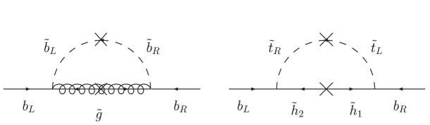
Figure 1: Dominant contributions to the bottom quark self energy at large $t_{\beta}$, in the single VEV insertion approximation.

We may then use the HLET to calculate the corresponding graphs with an additional zero momentum Higgs insertion. The lowest order $\phi_{S}b\bar{b}$ graphs are shown in Fig. 2. Neglecting again terms proportional to $\alpha_{w}$, the coupling parameters $\Delta_{b}^{\phi_{2,S}}$ are given by

$$\Delta_{b}^{\phi_{2}} = {2\alpha_{s}\over 3\pi}\;M_{3}\;\Bigg{[}\,\mu\;I(m^{2}_{\tilde{b}_{1}},m^{2}_{\tilde{b}_{2}},M^{2}_{3})\ -X_{b}v_{1}{\partial\over\partial\phi_{2}}\ I(m^{2}_{\tilde{b}_{1}},m^{2}_{\tilde{b}_{2}},M^{2}_{3})\,\Bigg{]}$$

$$+\ {h_{t}^{2}\over 16\pi^{2}}\;A_{t}\;\Bigg{[}\ m_{\tilde{\chi}_{1}}{\mathcal{V}}^{\dagger}_{21}{\mathcal{U}}^{\ast}_{12}\;I(m^{2}_{\tilde{t}_{1}},m^{2}_{\tilde{t}_{2}},m^{2}_{\tilde{\chi}_{1}})+m_{\tilde{\chi}_{2}}{\mathcal{V}}^{\dagger}_{22}{\mathcal{U}}^{\ast}_{22}\;I(m^{2}_{\tilde{t}_{1}},m^{2}_{\tilde{t}_{2}},m^{2}_{\tilde{\chi}_{2}})\Bigg{]}\$$

$$+\ {h_{t}^{2}\over 16\pi^{2}}\;X_{t}v_{2}\;{\partial\over\partial\phi_{2}}\Bigg{[}\ m_{\tilde{\chi}_{1}}{\mathcal{V}}^{\dagger}_{21}{\mathcal{U}}^{\ast}_{12}\;I(m^{2}_{\tilde{t}_{1}},m^{2}_{\tilde{t}_{2}},m^{2}_{\tilde{\chi}_{1}})+m_{\tilde{\chi}_{2}}{\mathcal{V}}^{\dagger}_{22}{\mathcal{U}}^{\ast}_{22}\;I(m^{2}_{\tilde{t}_{1}},m^{2}_{\tilde{t}_{2}},m^{2}_{\tilde{\chi}_{2}})\Bigg{]}\;,$$

$$\Delta_{b}^{\phi_{S}} = {2\alpha_{s}\over 3\pi}\;M_{3}\,\Bigg{[}\,\mu\;{v_{2}\over v_{S}}I(m^{2}_{\tilde{b}_{1}},m^{2}_{\tilde{b}_{2}},M^{2}_{3})\ -X_{b}v_{1}{\partial\over\partial\phi_{S}}\ I(m^{2}_{\tilde{b}_{1}},m^{2}_{\tilde{b}_{2}},M^{2}_{3})\,\Bigg{]}$$

$$-\ {h_{t}^{2}\over 16\pi^{2}}\;\mu{v_{1}\over v_{S}}\;\Bigg{[}\ m_{\tilde{\chi}_{1}}{\mathcal{V}}^{\dagger}_{21}{\mathcal{U}}^{\ast}_{12}\;I(m^{2}_{\tilde{t}_{1}},m^{2}_{\tilde{t}_{2}},m^{2}_{\tilde{\chi}_{1}})+m_{\tilde{\chi}_{2}}{\mathcal{V}}^{\dagger}_{22}{\mathcal{U}}^{\ast}_{22}\;I(m^{2}_{\tilde{t}_{1}},m^{2}_{\tilde{t}_{2}},m^{2}_{\tilde{\chi}_{2}})\Bigg{]}$$

$$+\ {h_{t}^{2}\over 16\pi^{2}}\;X_{t}v_{2}\;{\partial\over\partial\phi_{S}}\Bigg{[}\ m_{\tilde{\chi}_{1}}{\mathcal{V}}^{\dagger}_{21}{\mathcal{U}}^{\ast}_{12}\;I(m^{2}_{\tilde{t}_{1}},m^{2}_{\tilde{t}_{2}},m^{2}_{\tilde{\chi}_{1}})+m_{\tilde{\chi}_{2}}{\mathcal{V}}^{\dagger}_{22}{\mathcal{U}}^{\ast}_{22}\;I(m^{2}_{\tilde{t}_{1}},m^{2}_{\tilde{t}_{2}},m^{2}_{\tilde{\chi}_{2}})\Bigg{]}\;,$$

where $X_{b}=A_{b}-\mu t_{\beta}$ and $X_{t}=A_{t}-\mu/t_{\beta}$. The derivatives act on all Higgs-dependent functionals to their right, generating a rather lengthy expression which we do not show here explicitly. These derivative terms represent higher number of Higgs insertions, beyond the usual single Higgs insertion approximation often followed in the literature. They can be $t_{\beta}$-enhanced in certain regions of the parameter space, especially for the chargino case, and are therefore consistently included in our numerical analysis in Section 3.

The presence of the singlet in the model does not alter the 1-loop $\tan\beta$ enhanced couplings of the doublet Higgs fields well-known from the MSSM [14]. As a consistency check, we have compared the gluino-exchange terms of (2.1) with corresponding results from the first reference of [14], and we find that the HLET calculation gives identical results.

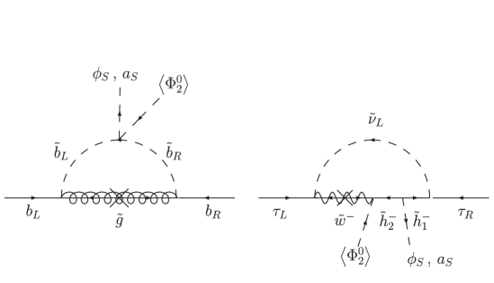
Figure 2: Dominant contributions to the couplings $\phi_{S}\bar{b}b$, $\phi_{S}\tau^{+}\tau^{-}$, $a_{S}\bar{b}b$ and $a_{S}\tau^{+}\tau^{-}$, in the large $t_{\beta}$ limit.

Correspondingly, the loop-induced coupling parameters $\Delta_{b}^{a_{2,S}}$ are given by

$$\Delta_{b}^{a_{2}} = {2\alpha_{s}\over 3\pi}\;M_{3}\;\,\mu\;I(m^{2}_{\tilde{b}_{1}},m^{2}_{\tilde{b}_{2}},M^{2}_{3})\,$$

$$+\ {h_{t}^{2}\over 16\pi^{2}}\;A_{t}\;\Bigg{[}\ m_{\tilde{\chi}_{1}}{\mathcal{V}}^{\dagger}_{21}{\mathcal{U}}^{\ast}_{12}\;I(m^{2}_{\tilde{t}_{1}},m^{2}_{\tilde{t}_{2}},m^{2}_{\tilde{\chi}_{1}})+m_{\tilde{\chi}_{2}}{\mathcal{V}}^{\dagger}_{22}{\mathcal{U}}^{\ast}_{22}\;I(m^{2}_{\tilde{t}_{1}},m^{2}_{\tilde{t}_{2}},m^{2}_{\tilde{\chi}_{2}})\Bigg{]}\$$

$$+\ {h_{t}^{2}\over 16\pi^{2}}\;X_{t}v_{2}\;{\partial\over\partial a_{2}}\Bigg{[}\ m_{\tilde{\chi}_{1}}{\mathcal{V}}^{\dagger}_{21}{\mathcal{U}}^{\ast}_{12}\;I(m^{2}_{\tilde{t}_{1}},m^{2}_{\tilde{t}_{2}},m^{2}_{\tilde{\chi}_{1}})+m_{\tilde{\chi}_{2}}{\mathcal{V}}^{\dagger}_{22}{\mathcal{U}}^{\ast}_{22}\;I(m^{2}_{\tilde{t}_{1}},m^{2}_{\tilde{t}_{2}},m^{2}_{\tilde{\chi}_{2}})\Bigg{]}\;,$$

$$\Delta_{b}^{a_{S}} = {2\alpha_{s}\over 3\pi}\;M_{3}\,\,\mu\;{v_{2}\over v_{S}}I(m^{2}_{\tilde{b}_{1}},m^{2}_{\tilde{b}_{2}},M^{2}_{3})$$

$$+\ {h_{t}^{2}\over 16\pi^{2}}\;\mu{v_{1}\over v_{S}}\;\Bigg{[}\ m_{\tilde{\chi}_{1}}{\mathcal{V}}^{\dagger}_{21}{\mathcal{U}}^{\ast}_{12}\;I(m^{2}_{\tilde{t}_{1}},m^{2}_{\tilde{t}_{2}},m^{2}_{\tilde{\chi}_{1}})+m_{\tilde{\chi}_{2}}{\mathcal{V}}^{\dagger}_{22}{\mathcal{U}}^{\ast}_{22}\;I(m^{2}_{\tilde{t}_{1}},m^{2}_{\tilde{t}_{2}},m^{2}_{\tilde{\chi}_{2}})\Bigg{]}$$

$$+\ {h_{t}^{2}\over 16\pi^{2}}\;X_{t}v_{2}\;{\partial\over\partial a_{S}}\Bigg{[}\ m_{\tilde{\chi}_{1}}{\mathcal{V}}^{\dagger}_{21}{\mathcal{U}}^{\ast}_{12}\;I(m^{2}_{\tilde{t}_{1}},m^{2}_{\tilde{t}_{2}},m^{2}_{\tilde{\chi}_{1}})+m_{\tilde{\chi}_{2}}{\mathcal{V}}^{\dagger}_{22}{\mathcal{U}}^{\ast}_{22}\;I(m^{2}_{\tilde{t}_{1}},m^{2}_{\tilde{t}_{2}},m^{2}_{\tilde{\chi}_{2}})\Bigg{]}\;,$$

Notice that both $\Phi_{2}^{0}$ and the singlet field $S$ enter the $b$-squark masses only through the mixing term $\left(A_{b}\Phi_{1}^{0}-\lambda S\Phi_{2}^{0}\right)$. As a result of this, it is easy to derive that $\partial m^{2}_{\tilde{b}_{i}}/\partial\phi_{S}=\left(v_{2}/v_{S}\right)\;\partial m^{2}_{\tilde{b}_{i}}/\partial\phi_{2}$. With the aid of the latter, we then find that $\Delta_{b}^{\phi_{2}}$ is related to $\Delta_{b}^{\phi_{S}}$ by $\Delta_{b}^{\phi_{S}}=\frac{v_{2}}{v_{S}}\;\Delta_{b}^{\phi_{2}}$, if the gluino-exchange diagram is only considered. In the same approximation, a similar relation holds true for the pseudoscalar 1-loop couplings: $\Delta_{b}^{a_{S}}=\frac{v_{2}}{v_{S}}\;\Delta_{b}^{a_{2}}$. However, this simple scaling behaviour is broken by the chargino-exchange diagram, as the background Higgs fields $\Phi^{0}_{2}$ and $S$ enter the chargino masses and mixing angles in a non-linear manner [cf. (A.2) and (A.2)].

Finally, it is worth commenting on the fact that the coupling of the neutral would-be Goldstone boson $G^{0}$ to the $b$ quark is proportional to the $b$-quark mass, as a consequence of a Ward identity involving the $Zb\bar{b}$-coupling. Specifically, the coupling parameter $\Delta_{b}^{G^{0}}$, which is computed by

$$\Delta_{b}^{G^{0}}\ =\ i\sqrt{2}\,\left<{\partial\over\partial G^{0}}\Delta_{b}\right>\ =\ i\sqrt{2}\,\left<\left(c_{\beta}{\partial\over\partial a_{1}}\ +\ s_{\beta}{\partial\over\partial a_{2}}\right)\Delta_{b}\right>\,,$$ (2.13)

is given by

$$\Delta_{b}^{G^{0}}\ =\ {\sqrt{2}\over v}\ \left<\Delta_{b}\right>\ .$$ (2.14)

Consequently, the $G^{0}b\bar{b}$-coupling has the tree-level SM form in the limit of zero external momentum.

2.2 Effective $\tau$-lepton Yukawa Couplings

The derivation of effective $\tau$-lepton Yukawa couplings goes along the lines discussed above for the $b$-quark case. At the one loop order, there is now only one $t_{\beta}$-enhanced diagram contributing to $\Delta_{\tau}$, which originates from the chargino-Higgsino-exchange diagram of Fig. 2. The effective functional $\Delta_{\tau}$ pertinent to the $\tau$-lepton self-energy is given by

$$\Delta_{\tau}=-{\alpha_{w}\over 4\pi}\Bigg{[}\;m_{\tilde{\chi}_{1}}{\mathcal{V}}^{\dagger}_{11}{\mathcal{U}}^{\ast}_{12}\;B_{0}\left(0,m_{\tilde{\chi}_{1}},M_{\widetilde{L}}\right)+\ m_{\tilde{\chi}_{2}}{\mathcal{V}}^{\dagger}_{12}{\mathcal{U}}^{\ast}_{22}\;B_{0}\left(0,m_{\tilde{\chi}_{2}},M_{\widetilde{L}}\right)\;\Bigg{]}\;,$$ (2.15)

where $M_{\widetilde{L}}$ is the soft SUSY-breaking mass term for the left-handed sleptons and the loop function $B^{0}(p^{2},a,b)$ at $p^{2}=0$ takes on the simple form

$$B_{0}(0,a,b)\ =\ -\,\ln\left({ab\over Q^{2}}\right)\ +\ 1\ +\ {a^{2}+b^{2}\over b^{2}-a^{2}}\ln\left({a^{2}\over b^{2}}\right)\;,$$ (2.16)

where $Q^{2}$ is the renormalization scale, which is conveniently taken to be $Q^{2}=m_{\tilde{\chi}_{2}}M_{\tilde{L}}$.

Notice that the non-holomorphic couplings both receive renormalization scale-dependent contributions. This should not be suprising, as the couplings also contain contributions from the mixing of $\phi_{2,S}$ with the holomorphic $\phi_{1}$. We have checked that all scale-dependent terms vanish in the zero mixing limit of $\phi_{2,S}\to\phi_{1}$, corresponding to $v_{1}\to 0$.

As was done above for the $b$-quark case, the 1-loop Higgs-boson couplings to $\tau^{+}\tau^{-}$ may be computed from (2.15) by means of the HLET, where the dominant $\phi_{S}\tau^{+}\tau^{-}$ diagram is shown in Fig. 2. In extensions that include right handed (s)neutrinos, a second diagram mediated by Higgsino exchange must also be considered. This new contribution may be significant if (s)neutrinos are not too heavy. Such further extensions may be studied elsewhere.

3 Phenomenological Discussion

In this section we analyze the implications of the loop-induced parameters $\Delta_{f}^{\phi_{S}}$ and $\Delta_{f}^{a_{S}}$ for the Higgs-boson couplings and for the Higgs-boson phenomenology in general. As was already mentioned, the 1-loop coupling of the singlet Higgs boson to the $b$ quark and the $\tau$ lepton becomes significant at large values of $\tan\beta$. In our analysis, we adopt a benchmark scenario where the singlet Higgs-boson effects get enhanced. Unless is stated otherwise, the default values of the SUSY parameters for our benchmark scenario are

$$\begin{array}[]{lll}\mu\ =\ \frac{1}{\sqrt{2}}\,\lambda\,v_{S}\ =\ 110~{}{\rm GeV},&t_{\beta}\ =\ 50,&\\ M_{\widetilde{Q}}\ =\ 300~{}{\rm GeV},&M_{\widetilde{L}}\ =\ 90~{}GeV,&\\ M_{\tilde{t}}\ =\ 600~{}{\rm GeV},&M_{\tilde{b}}\ =\ 110~{}{\rm GeV},&M_{\tilde{\tau}}\ =\ 200~{}{\rm GeV},\\ A_{t}\ =\ 1~{}{\rm TeV},&A_{b}\ =\ 1~{}{\rm TeV},&A_{\tau}\ =\ 1~{}{\rm TeV},\\ M_{1}\ =\ 400~{}{\rm GeV},&M_{2}\ =\ 600~{}{\rm GeV},&M_{3}\ =\ 400~{}{\rm GeV}\;.\end{array}$$ (3.1)

Notice that an important constraint on the choice of the above parameters comes from the LEP data. This constraint is included in our analysis.

Given the model parameters (3.1), the coupling-parameter ratios $\Delta^{\phi_{S}}_{f}/\Delta^{\phi_{2}}_{f}$ and $\Delta^{a_{S}}_{f}/\Delta^{a_{2}}_{f}$ are shown in Fig. 3, as functions of the supersymmetric coupling $\lambda$, keeping the $\mu$-parameter fixed. Since the radiative corrections to the Yukawa couplings are dominated by SUSY QCD effects in the case of the quarks, one might expect for the ratios to be approximately given by $\Delta^{\phi_{S}}_{b}/\Delta^{\phi_{2}}_{b}\approx\Delta^{a_{S}}_{b}/\Delta^{a_{2}}_{b}\approx v/v_{S}$. Specifically, this ratio should reach the value 1 for $\lambda\sim 0.65$. As is illustrated in Fig. 3, whilst this approximation is valid for the psuedoscalar couplings, the subdominant corrections to the scalar couplings do not share this simple scaling behaviour and so give rise to a somewhat different relative magnitude for $\Delta^{\phi_{S}}_{b}/\Delta^{\phi_{2}}_{b}$. Clearly, including interference effects between the contributing terms, the coupling parameter $\Delta^{\phi_{S}}_{b}$ becomes comparable with $\Delta^{\phi_{2}}_{b}$ only for large values of $\lambda$.

Figure 3: Numerical estimates of the ratios $\Delta^{\phi_{S}}_{b,\tau}/\Delta^{\phi_{2}}_{b,\tau}$ and $\Delta^{a_{S}}_{b,\tau}/\Delta^{a_{2}}_{b,\tau}$ as functions of $\lambda$. The values of the model parameters are given in (3.1).

As can be seen from the effective Lagrangian (2.3), the physical Higgs-boson couplings to the $b$ quark and the $\tau$ lepton, e.g. $H_{1,2,3}f\bar{f}$ and $A_{1,2}f\bar{f}$, consist of two contributions. The first contribution is the proper vertex interaction, which is dominated by the tree-level $\phi_{1}$-coupling. The second contribution is the mixing of the fields $\phi_{2,S}$ with the $\phi_{1}$. Such a mixing of Higgs states occurs at the tree level and is very significant for generic Higgs-boson mass matrices, as only a $2\%$ component of $\phi_{1}$ will give an effective $\phi_{2,S}$-coupling of order $h_{b}^{\rm SM}$ at $t_{\beta}=50$. Since our interest is to assess the significance of the 1-loop singlet-Higgs vertex effects, we will mainly focus on variants of the mnSSM and the NMSSM, where the mixing of $\phi_{1}$ with the other scalars is suppressed.

3.1 Decoupling via a Heavy Charged Higgs Boson

One way to switch off the Higgs-boson self-energy transitions $\phi_{1}\to\phi_{2,S}$ and/or $a_{1}\to a_{2,S}$ is to consider the decoupling of the states $\phi_{1}$ and $a_{1}$ via a heavy charged Higgs boson, with $M_{H^{\pm}}\stackrel{{\scriptstyle>}}{{{}_{\sim}}}M_{\rm SUSY}$. Although the decoupling of $\phi_{1}$ may be easily achieved within the MSSM for relatively large values of $\tan\beta$ [16], the situation becomes a bit more involved in its singlet extensions. In particular, for the CP-even Higgs sector, one has to arrange that both mass-matrix elements $\left(M_{S}^{2}\right)_{12}$ and $\left(M_{S}^{2}\right)_{13}$ vanish, which is more difficult. However, this difficulty is not present for the CP-odd Higgs sector, where the mass-matrix element $\left(M_{P}^{2}\right)_{12}$ could vanish for certain choices of the model parameters, thereby decoupling the CP-odd state $a_{1}$ from the rest of the mass spectrum.

3.1.1 Mixing in the mnSSM

Before we discuss the Higgs-mixing effects, we first give a brief overview of the Higgs sector of the mnSSM. The renormalizable part of the mnSSM superpotential is given by

$${\mathcal{W}}_{\rm mnSSM} = h_{l}\widehat{H}_{d}^{T}i\tau_{2}\widehat{L}\widehat{E}\ +\ h_{d}\widehat{H}_{d}^{T}i\tau_{2}\widehat{Q}\widehat{D}\ +\ h_{u}\widehat{Q}^{T}i\tau_{2}\widehat{H}_{u}\widehat{U}$$ (3.2)

$$+\;\lambda\widehat{S}\widehat{H}_{d}^{T}i\tau_{2}\widehat{H}_{u}\ +\ t_{F}\widehat{S}\;.$$

In (3.2) the term linear in $\widehat{S}$ is induced by supergravity quantum effects from Planck-suppressed non-renormalizable operators in the Kähler potential and superpotential. Depending on the discrete $R$ symmetries imposed on the theory, the effective tadpole parameter $t_{F}$ and its associate soft SUSY-breaking term $t_{S}\,S$ may be generated at loop levels higher than 5 and can both be of order $M_{\rm SUSY}$. These two interactions are essential to break the unwanted PQ symmetry. Further details related to the tadpole generation and the breaking of the PQ symmetry may be found in [15].

In the mnSSM, the tree-level CP-odd mass matrix $M_{P}^{2}$ reads

$$\left(M_{P}^{2}\right)_{11} = M_{a}^{2}\;,$$

$$\left(M_{P}^{2}\right)_{12} = {v\over v_{S}}\left(s_{\beta}c_{\beta}M_{a}^{2}\>+\>m_{12}^{2}\right)\;,$$

$$\left(M_{P}^{2}\right)_{22} = {v^{2}\over v^{2}_{S}}\left(s_{\beta}c_{\beta}M_{a}^{2}\>+\>m_{12}^{2}\right)\ +\ {\lambda t_{S}\over\mu}\ ,$$ (3.3)

where subscript 1 refers to the CP-odd state $a=-s_{\beta}a_{1}+c_{\beta}a_{2}$ and the subscript 2 to the CP-odd state $a_{S}$. Moreover, $M_{a}$ is the would-be MSSM pseudoscalar Higgs mass, related to the charged Higgs-boson mass by $M_{a}^{2}=M_{H^{\pm}}^{2}-M_{W}^{2}+{1\over 2}\lambda^{2}v^{2}$ at the tree level, and $m_{12}^{2}$ is related to the effective superpotential tadpole $t_{F}$ by $m_{12}^{2}=\lambda t_{F}$. It is important to comment that the dominant scalar top and bottom corrections to the CP-odd mass matrix $M^{2}_{P}$ can all be absorbed to $M_{a}$ and so do not modify its tree-level form.

Figure 4: Masses of the $H_{1}$ (solid line), $H_{2}$ (dashed line) and $A_{1}$ (dot-dashed line) bosons in the mnSSM with $\mu=110$ GeV, $\lambda t_{S}/\mu=150^{2}$ GeV² and $m_{12}^{2}=-0.5$ TeV². The values of other soft SUSY-breaking parameters are given in (3.1).

By analogy, the tree-level CP-even mass matrix $M^{2}_{S}$ is given by

$$\left(M^{2}_{S}\right)_{11} = c_{\beta}^{2}M_{Z}^{2}\>+\>s_{\beta}^{2}M_{a}^{2}\;,$$

$$\left(M^{2}_{S}\right)_{12} = -s_{\beta}c_{\beta}\left(M_{a}^{2}+M_{Z}^{2}-\lambda^{2}v^{2}\right)\;,$$

$$\left(M^{2}_{S}\right)_{13} = -{v\over v_{S}}\left(s_{\beta}^{2}c_{\beta}M_{a}^{2}+s_{\beta}m_{12}^{2}-2c_{\beta}\mu^{2}\right)\;,$$

$$\left(M^{2}_{S}\right)_{22} = s_{\beta}^{2}M_{Z}^{2}+c_{\beta}^{2}M_{a}^{2}\;,$$

$$\left(M^{2}_{S}\right)_{23} = -{v\over v_{S}}\left(s_{\beta}c_{\beta}^{2}M_{a}^{2}+c_{\beta}m_{12}^{2}-2s_{\beta}\mu^{2}\right)\;,$$

$$\left(M^{2}_{S}\right)_{33} = s_{\beta}c_{\beta}\left({v\over v_{S}}\right)^{2}\left(s_{\beta}c_{\beta}M_{a}^{2}+m_{12}^{2}\right)+{\lambda t_{S}\over\mu}\ ,$$ (3.4)

where the subscripts $1,2,3$ refer to the CP-even states $\phi_{1,2,S}$, respectively. In our numerical analysis we also include the 1-loop corrections to $M^{2}_{S}$ due to both (s)top and (s)bottom loops, which play an important role both for intermediate and large values of $t_{\beta}$.

To cancel the mixing of state $a_{1}$ with the other CP-odd Higgs states, we only need to choose $m_{12}^{2}$, such that it satisfies the relation

$$s_{\beta}c_{\beta}M_{a}^{2}\ +\ m_{12}^{2}\ =\ 0\;.$$ (3.5)

This relation also approximately cancels $\left(M_{S}^{2}\right)_{13}$ in the large $t_{\beta}$ limit. We shall enforce this constraint at all times when considering the mnSSM.

Figure 5: The SM-normalized couplings $H_{1}b\bar{b}$, $H_{2}b\bar{b}$ and $A_{1}b\bar{b}$ in the mnSSM, as functions of $\lambda$, for the same model parameters as in Fig. 4. Also shown are the corresponding couplings $H_{1}b\bar{b}$ and $H_{2}b\bar{b}$ with the singlet threshold correction $\Delta^{\phi_{S}}_{b}=0$ for comparison. The pseudoscalar couplings are approximately zero when $\Delta^{a_{S}}_{b}=0$.

In Fig. 4 we display the masses of the two lightest CP-even Higgs bosons $H_{1}$ and $H_{2}$ and the lightest CP-odd Higgs boson $A_{1}$. Since we have taken $M_{H^{\pm}}=5$ TeV and $\lambda t_{S}/\mu=150^{2}$ GeV², the remaining physical Higgs states, $H_{3}\sim\phi_{1}$ and $A_{2}\sim a$, are heavy of order $M_{H^{\pm}}$. We observe that the lightest Higgs boson mass $M_{H_{1}}$ goes well below the LEP limit from direct Higgs searches, for large values of $\lambda\stackrel{{\scriptstyle>}}{{{}_{\sim}}}0.3$. Hence, the coupling $\lambda$ has to be smaller than about 0.3 for a phenomenological viable model. In Fig. 5 we then show the dependence of the $b$-quark Yukawa couplings $g^{S}_{H_{1,2}bb}$ and $g^{P}_{A_{1}bb}$, for the aforementioned scenario. We find that the CP-even Yukawa couplings $g^{S}_{H_{1,2}bb}$ receive appreciable contributions from the tree-level mixing of the state $\phi_{1}$ with $\phi_{2,S}$, which is competitive to the loop-induced Yukawa couplings $\Delta^{\phi_{2,S}}_{b}$. On the other hand, the coupling $g^{P}_{A_{1}b\bar{b}}\approx g^{P}_{a_{S}b\bar{b}}$ is completely dominated by the 1-loop contribution $\Delta^{a_{S}}_{b}$. For moderate values of $\lambda\sim 0.3$, we find that $g^{P}_{A_{1}b\bar{b}}\sim 0.15$, so the $A_{1}\bar{b}b$-coupling is $\sim 15\%$ of the SM Higgs boson coupling to the $b$ quark. Moreover, the decay $A_{1}\to\bar{b}b$ is expected to be the dominant decay channel in this specific scenario of the mnSSM.

For completeness, we present numerical estimates for the effective Higgs-boson couplings to the $W^{\pm}$ and $Z$ bosons. These can be determined by the effective Lagrangian

$${\mathcal{L}}_{HVV}\ =\ g_{w}M_{W}\sum_{i=1}^{3}g_{H_{i}VV}\left(H_{i}W^{+}_{\mu}W^{-,\mu}\ +\ {1\over c_{w}^{2}}H_{i}Z_{\mu}Z^{\mu}\right)\;,$$ (3.6)

where $c_{w}=\sqrt{1-s_{w}^{2}}=M_{W}/M_{Z}$ and

$$g_{H_{i}VV}\ =\ O^{H}_{2i}\,c_{\beta}\>+\>O^{H}_{1i}\,s_{\beta}\;.$$ (3.7)

In the scenario of the mnSSM specified above, the SM-normalized couplings $g_{H_{1,2}VV}$ are shown in Fig. 6. Combining the results of this last figure with Figs. 4 and 5, we observe that both the lightest CP-even Higgs bosons $H_{1,2}$ will predominantly decay into $b$ quarks, for small values of $\lambda$, e.g. for $\lambda\sim 0.05$. For larger values, i.e. for $\lambda\stackrel{{\scriptstyle>}}{{{}_{\sim}}}0.1$, only the $H_{1}$ boson will decay into $b$ quarks, whereas the heavier one $H_{2}$ will decay into $W^{\pm}$ bosons.

Figure 6: Effective vector boson couplings for the Higgs bosons $H_{1}$ (solid line) and $H_{2}$ (dashed line) in the mnSSM, for the same model parameters as in Fig 4.

3.1.2 Mixing in the NMSSM

We now turn our attention to the NMSSM. The superpotential of this model is given by

$${\mathcal{W}}_{\rm NMSSM} = h_{l}\widehat{H}_{d}^{T}i\tau_{2}\widehat{L}\widehat{E}\>+\>h_{d}\widehat{H}_{d}^{T}i\tau_{2}\widehat{Q}\widehat{D}\>+\>h_{u}\widehat{Q}^{T}i\tau_{2}\widehat{H}_{u}\widehat{U}$$ (3.8)

$$+\>\lambda\widehat{S}\widehat{H}_{d}^{T}i\tau_{2}\widehat{H}_{u}\>+\>{\kappa\over 3}\widehat{S}^{3}\;.$$

The difference between the mnSSM and the NMSSM is that the effective tadpole parameter linear in $\widehat{S}$ in the former model is now replaced by an operator cubic in $\widehat{S}$. In addition to the superpotential term ${\kappa\over 3}\widehat{S}^{3}$, there will be a soft SUSY-breaking operator ${\kappa\over 3}\,A_{\kappa}S^{3}$, which needs be considered as well in the calculation of the Higgs-boson mass matrices.

In the same weak basis as the one considered for the mnSSM, we first present the CP-odd Higgs-boson mass matrix $M^{2}_{P}$. At the tree level, $M^{2}_{P}$ may be conveniently expressed as

$$\left(M_{P}^{2}\right)_{11} = M_{a}^{2}\;,$$

$$\left(M_{P}^{2}\right)_{12} = {v\over v_{S}}\left(s_{\beta}c_{\beta}M_{a}^{2}\>+\>3{\kappa\over\lambda}\mu^{2}\right)\;,$$

$$\left(M_{P}^{2}\right)_{22} = {v^{2}\over v_{S}^{2}}s_{\beta}c_{\beta}\left(s_{\beta}c_{\beta}M_{a}^{2}\>-\>3{\kappa\over\lambda}\mu^{2}\right)\ +\ 3{\kappa\over\lambda}\mu A_{\kappa}\;.$$ (3.9)

Here $s_{\beta}c_{\beta}M_{a}^{2}=\left(\mu A_{\lambda}-{\kappa\over\lambda}\mu^{2}\right)$ at tree level. In similar fashion, the individual matrix elements of the tree-level CP-even Higgs-boson mass matrix $M^{2}_{S}$ are written down as follows:

$$\left(M_{S}^{2}\right)_{11} = c_{\beta}^{2}M_{Z}^{2}\>+\>s_{\beta}^{2}M_{a}^{2}\;,$$

$$\left(M_{S}^{2}\right)_{12} = -\,s_{\beta}c_{\beta}\left(M_{a}^{2}\>+\>M_{Z}^{2}\>-\>\lambda^{2}v^{2}\right)\;,$$

$$\left(M_{S}^{2}\right)_{22} = s_{\beta}^{2}M_{Z}^{2}\>+\>c_{\beta}^{2}M_{a}^{2}\;,$$

$$\left(M_{S}^{2}\right)_{13} = -\,{v\over v_{S}}\,\left(s_{\beta}^{2}c_{\beta}M_{a}^{2}\>-\>2c_{\beta}\mu^{2}\>-\;{\kappa\over\lambda}\,s_{\beta}\mu^{2}\,\right)\;,$$

$$\left(M_{S}^{2}\right)_{23} = -{v\over v_{S}}\left(s_{\beta}c^{2}_{\beta}M_{a}^{2}\>-\>2s_{\beta}\mu^{2}\>-\>{\kappa\over\lambda}c_{\beta}\mu^{2}\right)\;,$$

$$\left(M_{S}^{2}\right)_{33} = {v^{2}\over v_{S}^{2}}\,s_{\beta}c_{\beta}\,\left(\,s_{\beta}c_{\beta}M_{a}^{2}\>+\>{\kappa\over\lambda}\,\mu^{2}\right)\>-\>{\kappa\over\lambda}\mu A_{\kappa}\>+\>4{\kappa^{2}\over\lambda^{2}}\mu^{2}\,.$$ (3.10)

Figure 7: The SM-normalized couplings $H_{1}b\bar{b}$ (solid line), $A_{1}b\bar{b}$ (dashed line) and $A_{1}\tau^{+}\tau^{-}$ (dot-dashed line) in the NMSSM, as functions of $\lambda$, where the parameters $\kappa$ and $A_{\kappa}$ are constrained by (3.11) and (3.13). We also show the coupling $H_{1}b\bar{b}$ with the singlet threshold correction $\Delta^{\phi_{s}}_{b}=0$. Both pseudoscalar couplings $A_{1}ff$ are approximately zero when $\Delta^{a_{s}}_{f}=0$.

Following the same rationale as in the mnSSM, we suppress the mixing of the CP-odd state $a\approx-a_{1}$ with $a_{S}$ by requiring that $\left(M^{2}_{P}\right)_{12}=0$. Hence, we find that

$${\kappa\over\lambda}\ =\ -\,{s_{\beta}c_{\beta}\over 3\mu^{2}}\,M_{a}^{2}\;.$$ (3.11)

Note that for positive $\lambda$, we must have negative $\kappa$ to fulfil the above constraint. Substituting (3.11) into the expression for $\left(M_{P}^{2}\right)_{22}$ given in (3.1.2), we get the mass for the lightest CP-odd Higgs boson $A_{1}$, i.e.

$$M^{2}_{A_{1}}\ =\ \left(M_{P}^{2}\right)_{22}\ =\ -\,3\,{\kappa\over\lambda}\;\mu\,\left[2\left(v\over v_{S}\right)^{2}s_{\beta}c_{\beta}\mu\>-\>A_{\kappa}\,\right]\;.$$ (3.12)

For our benchmark value of $\mu=110$ GeV and for moderate $\lambda\sim 0.6$ with $t_{\beta}=50$, the positivity condition on $M^{2}_{A_{1}}$ gives an upper bound on $A_{\kappa}\sim 5$ GeV. The simplest option would be to set $A_{\kappa}=0$. The mass of $A_{1}$ then strongly depends upon the value of $\lambda$, through the factor $v/v_{S}$. In order to examine the effect of the threshold corrections on very light singlets across a larger range of $\lambda$, we instead allow $A_{\kappa}$ to vary such that

$$2\left(v\over v_{S}\right)^{2}s_{\beta}c_{\beta}\mu\>-\>A_{\kappa}\ =\ 0.05\sim 0.06$$ (3.13)

This, together with the above constraint (3.11), gives a singlet pseudoscalar mass of $M_{A_{1}}=6\sim 9$ GeV for $M_{H^{\pm}}=2$ TeV, across the full range of $\lambda$. The couplings of $H_{1}$ to $b\bar{b}$ and of $A_{1}$ to both $b\bar{b}$ and $\tau^{+}\tau^{-}$ pairs are shown in Fig. 7. In this variant of the NMSSM, lightest CP-even Higgs-boson mass $M_{H_{1}}$ is within the range $120$–$140$ GeV across the full range of $\lambda$.

The condition (3.11) can be re-written as a constraint on the parameter $A_{\lambda}$,

$$A_{\lambda}=-2{\kappa\over\lambda}\mu={2s_{\beta}c_{\beta}\over 3\mu}M^{2}_{a}$$ (3.14)

In view of (3.14) it is clear that a singlet dominated light pseudoscalar is present in the NMSSM spectrum if $A_{\lambda}\sim 200$ GeV and $A_{\kappa}\sim 5$ GeV. This can be naturally arranged in gauge or gaugino mediated SUSY breaking scenarios, where $A_{\lambda}$ and $A_{\kappa}$ are zero at tree level. Quantum contributions from gaugino masses produce non-zero values at the one- and two-loop level respectively, leading to the approximate scales shown above if the gaugino masses are of the order $100$ GeV [11]. Although we have artificially set $(M_{P}^{2})_{12}$ exactly to zero in order to make the effect of the one-loop correction explicit, similar considerations apply to the more natural scenario of small but non-vanishing pseudoscalar mixing.

In the last years, there has been some interest in the phenomenology of light Higgs pseudoscalars, which may provide an invisible decay channel for a light SM-like Higgs boson. If these CP-odd scalars have a large singlet component, it is possible for them to escape experimental bounds [17]. It is clear that the threshold corrections can have a significant effect on the branching ratios of a light CP-odd singlet scalar for moderate to large values of $\lambda$. Previous studies have considered detection of these particles through decays to photon pairs as the dominant mode [18] in the limit of vanishing singlet-doublet pseudoscalar mixing. However, our analysis shows that this need not be the case, and the impact of the hadronic decays of $A_{1}$ in so-called “invisible Higgs” scenarios should still be considered even in this limit.

3.2 Decoupling by Tuning $\lambda$ in the mnSSM

In the mnSSM the turning off of the singlet-doublet mixing of the CP-odd Higgs scalars leads automatically to a suppression of the mass matrix element $(M^{2}_{S})_{13}$, which in turn implies a small mixing of $\phi_{1}$ with $\phi_{S}$. Nevertheless, it is also possible to decouple $\phi_{1}$ from the other CP-even Higgs state $\phi_{2}$ by tuning $\lambda$. Hence one may choose a value for $\lambda$, such that it is $(M^{2}_{S})_{12}=0$, or equivalently

$$-s_{\beta}c_{\beta}\left(M_{a}^{2}\>+\>M_{Z}^{2}\>-\>\lambda^{2}v^{2}\right)\>+\>\delta_{\rm rad}\ =\ 0\;,$$ (3.15)

where $\delta_{\rm rad}$ represents radiative corrections to the tree level mass matrix. Evidently, in the absence of any fundamental reason, such a scenario should be considered to be somewhat contrived, as it relies upon an unnatural cancellation of different terms to a relatively high level of precision.

Figure 8: Effective $b$-quark Yukawa couplings of the Higgs scalars $H_{1}$, $H_{3}$ and $A_{2}$, as functions of $\lambda t_{S}/\mu$ , where $\mu=110$ GeV, $M_{H^{\pm}}=120$ GeV, $m_{12}^{2}=-292$ GeV² and $\lambda=0.7895$. Also shown are the corresponding couplings $H_{1}b\bar{b}$ and $H_{3}b\bar{b}$ with the singlet threshold correction $\Delta_{b}^{\phi_{S}}=0$ for comparison. The pseudoscalar couplings are approximately zero when $\Delta_{b}^{a_{S}}=0$.

In Fig. 8 we present numerical estimates of the Yukawa couplings for this contrived model. As input values, we take $M_{H^{\pm}}=120$ GeV and $\lambda=0.7895$. The $b$-quark Yukawa couplings of $H_{1}\sim\phi_{2}$, $H_{3}\sim\phi_{S}$ and $A_{2}\sim a_{S}$ are plotted as functions of singlet mass parameter $\lambda t_{S}/\mu$. The threshold corrections are independent of the singlet mass scale $\lambda t_{S}/\mu$, so we expect a flat line when these dominate, as is the case for the CP-odd Higgs field $A_{2}$. Instead, the respective couplings of the CP-even Higgs bosons show a noticeable variation with increasing $\lambda t_{S}/\mu$, which originate from the fact that the mass matrix elements $(M^{2}_{S})_{13}$ and $(M^{2}_{S})_{23}$ do not exactly cancel in this contrived model. As a consequence, the Yukawa coupling constant $g_{H_{1}\bar{b}b}\sim g_{\phi_{2}\bar{b}b}$ receives an appreciable contribution thanks to the mixing between the doublets via an intermediate singlet state, i.e. $\phi_{2}\to\phi_{S}\to\phi_{1}$. Considering LEP constraints, this scenario of the mnSSM is only viable for heavy Higgs singlets with masses around 300 GeV.

4 Conclusions and Future Directions

Minimal extensions of the MSSM generically include singlet Higgs bosons. Although singlet Higgs bosons have no direct or proper couplings to the SM particles, their interaction with the observed matter can still be significant as a result of two contributions. The first one is their mixing with Higgs doublet states, which is the one often considered in the literature. The second contribution is novel and persists even if the Higgs doublet-singlet mixing is completely switched off. It results from gluino, chargino and squark quantum effects at the 1-loop level and has been the focus of this paper.

In this article we have derived an effective Lagrangian which describes the interactions between the Higgs bosons and the down-type quarks and leptons in CP-conserving singlet extensions of the MSSM. We have found that the loop-induced singlet Higgs-boson couplings are enhanced for large values of $\tan\beta\stackrel{{\scriptstyle>}}{{{}_{\sim}}}40$. We have examined the effects of these couplings on the phenomenology of two such models, the mnSSM and the NMSSM. Although the mixing of $\phi_{1}$ with the other CP-even Higgs scalars $\phi_{2,S}$ is the leading effect for most of the parameter space, we have found that the threshold corrections to the Yukawa couplings remain relevant and can play an important role in the phenomenology of possibly light singlet Higgs scalars.

In the absence of a Higgs doublet-singlet mixing, the 1-loop quantum effects we have been studying here will be the only means by which the CP-odd singlet may couple to quarks and leptons. For a sufficiently light CP-odd singlet scalar, with a mass below the squark threshold, the loop-induced Yukawa couplings will provide its dominant decay channel into $b$ quarks. This has important phenomenological implications, since a SM-like Higgs boson will no longer decay invisibly into a pair of light singlet pseudoscalars $A_{1}A_{1}$. The threshold corrections that we calculated here will give rise to the leading decay mode $A_{1}\to b\bar{b}$. In fact, this decay channel depends on the mass of $A_{1}$, and can have a coupling strength of up to $\sim 1/2$ of the corresponding SM coupling, i.e. $g^{P}_{A_{1}bb}\sim 0.5$.

There are several possible new directions for future study. For instance, one may lift the assumption of CP conservation in the singlet extensions of the MSSM. Then, light CP-odd scalars may contribute to electron and neutron electric dipole moments at the 2-loop level [19]. It would be interesting to study the impact of those contributions in the presence of CP-violating threshold corrections. Another possible direction for future investigations will be to calculate the off-diagonal couplings of the singlet Higgs bosons to down-type quarks [20]. Our effective Lagrangian presented here may be generalized to include these flavour-changing neutral-current (FCNC) interactions of the Higgs bosons to quarks. It would be particularly valuable to explore the impact of the singlet Higgs-boson FCNC effects on $K$- and $B$-meson observables.

Acknowledgements

This work is supported in part by the PPARC research grant: PP/D000157/1.

Appendix A Background-Field-Dependent Masses and Mixing Angles

In this appendix we present our notation and conventions for the masses and mixing angles which enter the calculations of Sections 2.1 and 2.2. We have divided the appendix into two subsections. The first gives the relevant squark mass parameters, whilst the second contains the corresponding information for the chargino sector.

A.1 Squark Masses and Mixing Angles

Neglecting D-term contributions, the scalar top and bottom mass matrices may be written in the $(\tilde{q}_{L},\tilde{q}_{R})^{T}$ basis as

$$\widetilde{\mathcal{M}}^{2}_{t}=\left(\begin{array}[]{cc}\tilde{M}_{Q}^{2}+h_{t}^{2}|\Phi_{2}^{0}|^{2}&h_{t}A_{t}\Phi_{2}^{0\ast}-h_{t}\lambda S\Phi_{1}^{0\ast}\\ h_{t}A_{t}\Phi_{2}^{0}-h_{t}\lambda S^{\ast}\Phi_{1}^{0}&\tilde{M}_{t}^{2}+h_{t}^{2}|\Phi_{2}^{0}|^{2}\end{array}\right)\;,$$ (A.1)

$$\widetilde{\mathcal{M}}^{2}_{b}=\left(\begin{array}[]{cc}\tilde{M}_{Q}^{2}+h_{b}^{2}|\Phi_{1}^{0}|^{2}&h_{b}A_{b}\Phi_{1}^{0}-h_{b}\lambda S\Phi_{2}^{0}\\ h_{b}A_{b}\Phi_{1}^{0\ast}-h_{b}\lambda S^{\ast}\Phi_{2}^{0\ast}&\tilde{M}_{b}^{2}+h_{b}^{2}|\Phi_{1}^{0}|^{2}\end{array}\right)\;.$$ (A.2)

Where the fields $\Phi_{i}^{0}$ and $S$ have been defined after (2.1). These matrices are diagonalized by unitary matrices which may be parameterised as

$$\left(\begin{array}[]{c}\tilde{q}_{L}\\ \tilde{q}_{R}\end{array}\right)=\left(\begin{array}[]{cc}\cos\theta_{q}&\sin\theta_{q}\\ -\sin\theta_{q}&\cos\theta_{q}\end{array}\right)\left(\begin{array}[]{cc}1&0\\ 0&e^{i\delta_{q}}\end{array}\right)\left(\begin{array}[]{c}\tilde{q}_{1}\\ \tilde{q}_{2}\end{array}\right)\;,$$ (A.3)

where

$$\delta_{q} = \arg\left(\left(\widetilde{\mathcal{M}}_{q}^{2}\right)_{12}\right)\;,$$

$$s_{t}\equiv\sin\theta_{t} = \sqrt{m^{2}_{\tilde{t}_{2}}-\tilde{M}_{Q}^{2}-h_{t}^{2}|\Phi_{2}^{0}|^{2}\over m^{2}_{\tilde{t}_{2}}-m^{2}_{\tilde{t}_{1}}}\;,$$

$$s_{b}\equiv\sin\theta_{b} = \sqrt{m^{2}_{\tilde{b}_{2}}-\tilde{M}_{Q}^{2}-h_{b}^{2}|\Phi_{1}^{0}|^{2}\over m^{2}_{\tilde{b}_{2}}-m^{2}_{\tilde{b}_{1}}}\;,$$ (A.4)

and $c_{q}\equiv\cos\theta_{q}=\sqrt{1-s_{q}^{2}}$.

The field-dependent scalar quark masses are given by

$$\tilde{m}^{2}_{t_{1(2)}} = {1\over 2}\left[\tilde{M}_{Q}^{2}+\tilde{M}_{t}^{2}+2h_{t}^{2}|\Phi_{2}^{0}|^{2}+(-)\sqrt{\left(\tilde{M}_{Q}^{2}-\tilde{M}_{t}^{2}\right)^{2}+4h_{t}^{2}|A_{t}\Phi_{2}^{0}-\lambda S^{\ast}\Phi_{1}^{0}|^{2}}\right]\;,$$ (A.5)

$$\tilde{m}^{2}_{b_{1(2)}} = {1\over 2}\left[\tilde{M}_{Q}^{2}+\tilde{M}_{b}^{2}+2h_{b}^{2}|\Phi_{1}^{0}|^{2}+(-)\sqrt{\left(\tilde{M}_{Q}^{2}-\tilde{M}_{b}^{2}\right)^{2}+4h_{b}^{2}|A_{b}\Phi_{1}^{0}-\lambda S\Phi_{2}^{0}|^{2}}\right]\;.$$ (A.6)

A.2 Chargino Masses and Mixing Angles

The Lagrangian describing the chargino masses and their Yukawa interactions to Higgs bosons is given by

$$-\,\mathcal{L}_{\chi}^{\pm}\ =\ \left(-i\tilde{w}_{L}^{-},\tilde{h}_{1L}^{-}\right)\;M\;\left(\begin{array}[]{c}-i\tilde{w}_{L}^{+}\\ \tilde{h}_{2L}^{+}\end{array}\right)\>+\>{\rm h.c.},$$ (A.7)

with

$$M\ =\ \left(\begin{array}[]{cc}M_{2}&g_{w}\Phi^{0*}_{2}\\ g_{w}\Phi^{0}_{1}&\lambda S\end{array}\right)\;.$$ (A.8)

The mass matrix $M$ may be diagonalized by the bi-unitary transformation

$$M_{D}\ =\ {\mathcal{U}}^{\ast}\,M\,{\mathcal{V}}^{\dagger}\;,$$ (A.9)

where $M_{D}={\rm diag}(m_{\chi_{1}},m_{\chi_{2}})$. Both the chargino masses and the elements of the unitary matrices ${\mathcal{U}}$ and ${\mathcal{V}}$ depend explicitly on the Higgs background fields $\Phi^{0}_{1,2}$ and $S$.

We may parameterise the unitary matrices ${\mathcal{U}},\;{\mathcal{V}}$ as

$${\mathcal{U}}^{\ast}\ =\ \left(\begin{array}[]{cc}\cos\theta^{-}&-\sin\theta^{-}\\ \sin\theta^{-}&\cos\theta^{-}\end{array}\right)\;\left(\begin{array}[]{cc}1&0\\ 0&e^{i\delta^{-}}\end{array}\right)\;,$$ (A.14)

$${\mathcal{V}}\ =\ \left(\begin{array}[]{cc}\cos\theta^{+}&-\sin\theta^{+}\\ \sin\theta^{+}&\cos\theta^{+}\end{array}\right)\;\left(\begin{array}[]{cc}1&0\\ 0&e^{i\delta^{+}}\end{array}\right)\;,$$ (A.19)

with

$$\delta^{-}\! \equiv \!\arg\left(M_{2}\Phi_{1}^{0\ast}+\lambda S^{\ast}\Phi_{2}^{0\ast}\right)\ ,$$

$$\delta^{+}\! \equiv \!\arg\left(M_{2}\Phi_{2}^{0\ast}+\lambda S\Phi_{1}^{0\ast}\right)\ ,$$

$$s^{-}\! \equiv \!\sin\theta^{-}\ =\ \sqrt{m_{\chi_{1}}^{2}-M_{2}^{2}-\frac{1}{4}\,g_{w}^{2}|\Phi^{0}_{2}|^{2}\over m^{2}_{\chi_{2}}-m^{2}_{\chi_{1}}}\ ,$$

$$s^{+}\! \equiv \!\sin\theta^{+}\ =\ \sqrt{m_{\chi_{1}}^{2}-M_{2}^{2}-\frac{1}{4}g_{w}^{2}|\Phi_{1}^{0}|^{2}\over m^{2}_{\chi_{2}}-m^{2}_{\chi_{1}}}\ ,$$ (A.20)

and $c^{\pm}\equiv\cos\theta^{\pm}=\sqrt{1-(s^{\pm})^{2}}$. The chargino masses are given by

$$m^{2}_{\tilde{\chi}_{2(1)}} = {1\over 2}\left[M_{2}^{2}+\lambda^{2}|S|^{2}+2g_{w}^{2}\left(|\Phi_{1}^{0}|^{2}+|\Phi_{2}^{0}|^{2}\right)\right.$$

$$\left.+(-)\sqrt{\left(M_{2}^{2}+\lambda^{2}|S|^{2}+2g_{w}^{2}\left(|\Phi_{1}^{0}|^{2}+|\Phi_{2}^{0}|^{2}\right)\right)^{2}-4|M_{2}\lambda S-2g_{w}\Phi_{1}^{0}\Phi_{2}^{0\ast}|^{2}}\right]\;.$$

References

- [1] S. Schael et al., Eur. Phys. J. C 47 (2006) 547 [arXiv:hep-ex/0602042].
-
[2]
J. E. Kim and H. P. Nilles,
Phys. Lett. B 138 (1984) 150;
L. J. Hall, J. D. Lykken and S. Weinberg, Phys. Rev. D 27, 2359 (1983);
G. F. Giudice and A. Masiero, Phys. Lett. B 206, 480 (1988);
E. J. Chun, J. E. Kim and H. P. Nilles, Nucl. Phys. B 370, 105 (1992);
I. Antoniadis, E. Gava, K. S. Narain and T. R. Taylor, Nucl. Phys. B 432, 187 (1994). - [3] E. Accomando et al., arXiv:hep-ph/0608079.
-
[4]
P. Fayet,
Nucl. Phys. B 90 (1975) 104;
J. M. Frere, D. R. T. Jones and S. Raby, Nucl. Phys. B 222 (1983) 11;
J. P. Derendinger and C. A. Savoy, Nucl. Phys. B 237 (1984) 307;
J. R. Ellis, J. F. Gunion, H. E. Haber, L. Roszkowski and F. Zwirner, Phys. Rev. D 39 (1989) 844;
S. F. King and P. L. White, Phys. Rev. D 52 (1995) 4183 [arXiv:hep-ph/9505326];
M. Bastero-Gil, C. Hugonie, S. F. King, D. P. Roy and S. Vempati, Phys. Lett. B 489, 359 (2000) [arXiv:hep-ph/0006198];
U. Ellwanger, J. F. Gunion and C. Hugonie, JHEP 0507 (2005) 041 [arXiv:hep-ph/0503203]. -
[5]
C. Panagiotakopoulos and A. Pilaftsis,
Phys. Rev. D 63 (2001) 055003
[arXiv:hep-ph/0008268];
A. Dedes, C. Hugonie, S. Moretti and K. Tamvakis, Phys. Rev. D 63 (2001) 055009 [arXiv:hep-ph/0009125];
A. Menon, D. E. Morrissey and C. E. M. Wagner, Phys. Rev. D 70 (2004) 035005 [arXiv:hep-ph/0404184];
S. W. Ham, S. K. OH, C. M. Kim, E. J. Yoo and D. Son, Phys. Rev. D 70 (2004) 075001 [arXiv:hep-ph/0406062]. -
[6]
M. Cvetic, D. A. Demir, J. R. Espinosa, L. L. Everett and P. Langacker,
Phys. Rev. D 56, 2861 (1997)
[Erratum-ibid. D 58, 119905 (1998)];
P. Langacker and J. Wang, Phys. Rev. D 58, 115010 (1998) [arXiv:hep-ph/9804428];
S. F. King, S. Moretti and R. Nevzorov, Phys. Rev. D 73 (2006) 035009 [arXiv:hep-ph/0510419]. -
[7]
J. Erler, P. Langacker and T. j. Li,
Phys. Rev. D 66, 015002 (2002);
V. Barger, P. Langacker, H. S. Lee and G. Shaughnessy, Phys. Rev. D 73 (2006) 115010. -
[8]
T. Banks,
Nucl. Phys. B 303 (1988) 172;
E. Ma, Phys. Rev. D 39 (1989) 1922. -
[9]
R. Hempfling,
Phys. Rev. D 49 (1994) 6168;
L. J. Hall, R. Rattazzi and U. Sarid, Phys. Rev. D 50 (1994) 7048 [arXiv:hep-ph/9306309];
M. Carena, M. Olechowski, S. Pokorski and C. E. M. Wagner, Nucl. Phys. B 426 (1994) 269 [arXiv:hep-ph/9402253];
D. M. Pierce, J. A. Bagger, K. T. Matchev and R. j. Zhang, Nucl. Phys. B 491 (1997) 3 [arXiv:hep-ph/9606211];
F. Borzumati, G. R. Farrar, N. Polonsky and S. D. Thomas, Nucl. Phys. B 555 (1999) 53 [arXiv:hep-ph/9902443]. -
[10]
J. A. Coarasa, R. A. Jimenez and J. Sola,
Phys. Lett. B 389 (1996) 312
[arXiv:hep-ph/9511402];
R. A. Jimenez and J. Sola, Phys. Lett. B 389 (1996) 53 [arXiv:hep-ph/9511292];
K. T. Matchev and D. M. Pierce, Phys. Lett. B 445 (1999) 331 [arXiv:hep-ph/9805275];
P. H. Chankowski, J. R. Ellis, M. Olechowski and S. Pokorski, Nucl. Phys. B 544 (1999) 39 [arXiv:hep-ph/9808275];
K. S. Babu and C. F. Kolda, Phys. Lett. B 451 (1999) 77 [arXiv:hep-ph/9811308]. -
[11]
R. Dermisek and J. F. Gunion,
Phys. Rev. Lett. 95 (2005) 041801;
Phys. Rev. D 73 (2006) 111701; hep-ph/0611142;
S. Chang, P. J. Fox and N. Weiner, JHEP 0608 (2006) 068 [arXiv:hep-ph/0511250]. -
[12]
J. R. Ellis, M. K. Gaillard and D. V. Nanopoulos,
Nucl. Phys. B 106 (1976) 292;
M. A. Shifman, A. I. Vainshtein and V. I. Zakharov, Phys. Lett. B 78 (1978) 443;
M. A. Shifman, A. I. Vainshtein, M. B. Voloshin and V. I. Zakharov, Sov. J. Nucl. Phys. 30 (1979) 711 [Yad. Fiz. 30 (1979) 1368];
A. I. Vainshtein, V. I. Zakharov and M. A. Shifman, Sov. Phys. Usp. 23 (1980) 429 [Usp. Fiz. Nauk 131 (1980) 537];
M. B. Voloshin, Sov. J. Nucl. Phys. 44 (1986) 478 [Yad. Fiz. 44 (1986) 738];
M. A. Shifman, Phys. Rept. 209 (1991) 341 [Sov. Phys. Usp. 32 (1989 UFNAA,157,561-598.1989) 289];
S. Dawson and H. E. Haber, Int. J. Mod. Phys. A 7 (1992) 107;
B. A. Kniehl and M. Spira, Z. Phys. C 69 (1995) 77 [arXiv:hep-ph/9505225]. - [13] D. Binosi, J. Papavassiliou and A. Pilaftsis, Phys. Rev. D 71 (2005) 085007 [arXiv:hep-ph/0501259].
-
[14]
M. Carena, D. Garcia, U. Nierste and C. E. M. Wagner,
Nucl. Phys. B 577 (2000) 88
[arXiv:hep-ph/9912516];
M. E. Gomez, T. Ibrahim, P. Nath and S. Skadhauge, Phys. Rev. D 74 (2006) 015015 [arXiv:hep-ph/0601163];
A. J. Buras, P. H. Chankowski, J. Rosiek and L. Slawianowska, Nucl. Phys. B 659 (2003) 3 [arXiv:hep-ph/0210145]. - [15] For a power-counting calculation of the size of the effective tadpole in the mnSSM, see the first reference in [5].
- [16] M. Carena, S. Mrenna and C. E. M. Wagner, Phys. Rev. D 62 (2000) 055008 [arXiv:hep-ph/9907422].
- [17] J. F. Gunion, D. Hooper and B. McElrath, Phys. Rev. D 73 (2006) 015011 [arXiv:hep-ph/0509024].
-
[18]
B. A. Dobrescu, G. Landsberg and K. T. Matchev,
Phys. Rev. D 63 (2001) 075003
[arXiv:hep-ph/0005308];
A. Arhrib, K. Cheung, T. J. Hou and K. W. Song, arXiv:hep-ph/0606114; arXiv:hep-ph/0611211. -
[19]
D. Chang, W. Y. Keung and A. Pilaftsis,
Phys. Rev. Lett. 82 (1999) 900
[arXiv:hep-ph/9811202];
A. Pilaftsis, Nucl. Phys. B 644 (2002) 263 [arXiv:hep-ph/0207277]. -
[20]
For a discussion of the FCNC coupling
in the NMSSM, where only the chargino-exchange diagram has been
considered and resummation of -enhanced terms has been
neglected, see,
G. Hiller, Phys. Rev. D 70 (2004) 034018 [arXiv:hep-ph/0404220].