Abstract

Basing upon dual analytic models, we present arguments in favor of the parametrization of generalized parton distributions (GPD) in the form $\sim(x/g_{0})^{(1-x)\tilde{\alpha}(t)},$ where $\tilde{\alpha}(t)=\alpha(t)-\alpha(0)$ is the nonlinear part of the Regge trajectory and $g_{0}$ is a parameter, $g_{0}>1.$ For linear trajectories it reduces to earlier proposals. We compare the calculated moments of these GPD with the experimental data on form factors and find that the effects from the nonlinearity of Regge trajectories are large. By Fourier-transforming the obtained GPD, we access the spatial distribution of protons in the transverse plane. The relation between dual amplitudes with Mandelstam analyticity and composite models in the infinite momentum frame is discussed, the integration variable in dual models being associated with the quark longitudinal momentum fraction $x$ in the nucleon.

$\begin{array}[]{ll}{}^{\star}\mbox{{\it e-mail address:}}&\mbox{jenk@bitp.kiev.ua}\end{array}$

1 Introduction

Generalized parton distributions (GPD) [1, 2, 3] combine our knowledge about the one-dimensional parton distribution in the longitudinal momentum with the impact-parameter, or transverse distribution of matter in a hadron or nucleus. It is an ambitious program to access the spatial distribution of partons in the transverse plane and thus to provide a 3-dimensional picture of the nucleon (nucleus) [4, 5, 6, 7, 8]. This program involves various approaches, including perturbative QCD, Regge poles, lattice calculations etc. (see Ref. [9] for reviews). The main problem is that, while the partonic subprocess can be calculated perturbatively, the calculation of GPDs require non-perturbative methods. GPDs enter in hard exclusive processes, such as deeply virtual Compton scattering (DVCS); however, they cannot be measured directly but instead appear in convolution integrals, that cannot be easily converted. Hence the strategy is to guess the GPD, based on various theoretical constraints, and then compare it with the data. In the first approximation, the GPD is proportional to the imaginary part of a DVCS amplitude, therefore, as discussed in [10], the knowledge (or experimental reconstruction) of the DVCS amplitude may partly resolve the problem, provided the phase of the DVCS amplitude is also known. In other words, a GPD can be viewed as the imaginary part of an antiquark-nucleon scattering amplitude, or a quark-nucleon amplitude in the $u$ channel.

Alternatively, one can extract [11, 12], still in a model-dependent way, the nontrivial interplay between the $x$ and $t$ dependence of GPD from light-cone wave functions

$$H(x,\xi=0,t)=\int d^{2}{\bf k}_{\bot}\psi^{*}(x,{\bf k}_{\bot})\psi(x,{\bf k}_{\bot})+(1-x){\bf q}_{\bot}),$$

where $\psi(x,{\bf k}_{\bot})$ is a 2-particle wave function (see, e.g., [13]) and $t\equiv{\bf q}_{\bot}.$

In two recent papers [14, 15] various forms of GPD for $\xi=0$ were tested against the experimental data on the related form factors. The agreement with the data in Ref.[14] is impressive; in Ref.[15] the spatial distribution of partons in the transverse plane was also calculated. We pursue the approach of Refs. [14, 15] by bringing more arguments coming from duality in favor of the parametrization for $H(x,t)$ used in [14] and exploring how analyticity and unitarity affect the $t$ dependence of GPD, the observable form factors and the calculated distribution of partons in the longitudinal and transverse planes. The effects are very large. Similarly to papers [14, 15], we limit ourselves the case of vanishing skewedness, $\xi=0.$

Regge trajectories play a key role in this analyses. Actually, there are two groups of trajectories in the problem: one, the $\rho,$ $\omega$ etc. trajectories exchanged in the valence quark distribution function ${\cal H}(x,t)$ (or, equivalently, the imaginary part of the $\bar{q}p$ scattering amplitude). Less evident are the characteristics of the corresponding trajectory in ”magnetic” densities ${\cal E}(x,t)$ for they cannot be expressed in terms of any known parton distribution. In Ref. [15] the $\rho$ trajectory, $\alpha_{\rho}(t)=0.48+0.88t,$ was fitted to the masses of $\rho(770)$ and $\rho_{3}(1690)$ and $\alpha_{\omega}(t)=0.42+0.95t$ to $\omega(782)$ and $\omega(1690)$. In [14], instead, the slopes of the trajectories in ${\cal H}(x,t)$ and ${\cal E}(x,t)$ were fitted to the data on form factors and are equal to $1.098$ GeV² and $1.158$ GeV${}^{2},$ respectively. The relevant intercepts are contained in the quark distributions, as discussed in Sec. 5. The resulting GPDs and related observables are very sensitive to the above parameters (see Fig. 1 in Ref.[14]). Even more sensitive are they to any deviation from linear trajectories, as shown in Sec. 6.

One can start either from trajectories fitted to resonances and scattering data (parametrizations of non-linear complex mesonic trajectories fitting the spectra of resonances as well scattering data exist in the literature [16, 17]) or treat them as ”effective” ones, to be fitted to the data on form factors. Our strategy here is to start from trajectories close to those in [14] (fitted to form factors) and then look for the effects coming from the deviations from linearity.

The paper is organized as follows. In Sec. 2, following earlier publications, we show how dual models with Mandelstam analyticity can be related to deep inelastic scattering and GPD. Regge trajectories satisfying the analyticity and unitarity constrains are introduced in Secs. 2 and 3, where their role in the calculation of form factors is also discussed. The relation between GPD and form factors is discussed of Sec. 4. A particular model of GPD with its $t$ dependence determined by dual models with Mandelstam analyticity, introduced in Sec. 2, is discussed in Sec. 5. Numerical calculations (form factors and parton distributions) are presented in Sec. 6. Our (temporary) conclusions and a discussion can be found in Section 7.

2 Non-linear Regge trajectories
in dual and composite models

Dual Amplitudes with Mandelstam analyticity (DAMA) were suggested (see [18] and earlier references therein) as a way to solve the manifestly non-unitarity of narrow-resonance dual models [19]. The $(u,t)$ term of the crossing-symmetric DAMA is

$$D(u,t)=\int_{0}^{1}{dx\biggl{(}{x\over g_{1}}\biggr{)}^{-\alpha(t(1-x))-1}\biggl{(}{1-x\over g_{2}}\biggr{)}^{-\alpha(ux)-1}},$$ (1)

where $u$ and $t$ are the Mandelstam variables, and $g_{1},\ g_{2}$ are parameters, $g_{1},g_{2}>1.$ In what follows we set, for simplicity, $g_{1}=g_{2}=g_{0}$. Similar expressions are valid for the $(st)$ and $(su)$ terms. They are not unique since the integrand of (1) can be multiplied by functions of the type $f(t(1-x))f(ux).$ Furthermore, the powers in the integrand can be shifted by integers determined by the quantum numbers of a particular reaction and relevant exchanges.

The functions $\alpha(y,x)),\ \ y=s,\ t,\ u,$ called in [18] homotopies, map the physical Regge trajectories $\alpha(y)$ onto linear functions $a+by$. Contrary to the narrow-resonance (=linear trajectories) Veneziano amplitude [19], applicable only to soft collisions of extended objects (strings), and decreasing exponentially at any scattering angle, DAMA does not only allow for, but even requires the use of nonlinear Regge trajectories. It will be convenient to write $\alpha(y)=\alpha(0)+\tilde{\alpha}(y),$ where $\tilde{\alpha}(y)$ will denote the nonlinear part of the trajectory.

For $|u|\rightarrow\infty$ and fixed $t,$ DAMA is Regge-behaved

$$D(u,t)\simeq g_{0}^{2}(-g_{0}u)^{\alpha(t)}[G(t)+...],$$

where

$$G(t)=\int_{0}^{\infty}dyy^{-y}y^{-\alpha(t)-1},$$

provided [18]

$$\left|{\alpha(u)\over{\sqrt{u}\ln u}}\right|\mathop{\leq}\limits_{u\to\infty}const,$$

which is equivalent to saying that the real part of the trajectory is bounded . Compatibility with the wide-angle scaling behavior of the amplitude, typical of point-like constituents, lowers this growth to a logarithm. Examples will be presented below.

The pole structure of DAMA

$$D(u,t)\sim\sum_{l=0}^{n}{C_{n-l}(t)\over{[n-\alpha(u)]^{l+1}}},$$ (2)

where $C_{n-l}(t)$ is the residue, whose form is fixed by the dual amplitude (see [18]), is similar to that of the Veneziano model except that multiple poles appear on daughter levels [18]. The pole term (2) in DAMA, comprising a whole sequence of resonances lying on a complex trajectory $\alpha(u),$ is a generalization of the Breit-Wigner formula. Such a ”reggeized” Breit-Wigner model has little practical use in the case of linear trajectories, resulting in an infinite sequence of poles, but it becomes a powerful tool in case of complex trajectories with a limited real part and hence a limited number of resonances.

The threshold behavior of DAMA satisfying the unitarity constrains [22]

$$D(u,t)\mathop{\sim}\limits_{t\to t_{0}}\sqrt{t-t_{0}}[const+\ln(1-t_{0}/t)],$$

is correlated with that of the trajectories [18],

$$\Im\alpha(t)\mathop{\sim}\limits_{t\to t_{0}}(t-t_{0})^{\alpha(t_{0})+1/2}.$$

For a light threshold this is close to the square-root behaviour to be used below.

A simple model, compatible both with to the above threshold behavior and with the Regge asymptotics (or polynomial boundedness) of the amplitude, yet fitting the data on resonances spectra, can be made of a sum of square roots (the assignment of the signs is uniquely determined by the requirement of positivity of the imaginary part etc., see [21]) [23]

$$\alpha(t)=\alpha(0)-\sum_{i}\alpha_{i}(\sqrt{t_{i}-t}-\sqrt{t_{i}}).$$ (3)

Linear trajectories appear as the limiting case of an infinitesimally heavy threshold $t_{1}\rightarrow\infty$ in

$$\alpha(t)=\alpha_{0}-\alpha_{1}(\sqrt{t_{1}-t}-\sqrt{t_{1}})$$

with fixed forward slope of the trajectory $\alpha^{\prime}={\alpha_{1}\over{2\sqrt{t_{i}}}}$. The limit of the infinitely rising linear trajectory is associated with a hadronic string, while the finite value of $t_{i}$ can be interpreted as a barrier where the string breaks (its tension ${1\over\alpha^{\prime}(t)}$ vanishes as $t\rightarrow t_{i},$ producing new particles instead of heavier resonances, see also [25]).

The number of thresholds is model-dependent: while the lightest one gives the dominant contribution to the imaginary part, those heavier promote the rise of the real part, terminating at the heaviest threshold.

To illustrate the aforesaid, a toy model can be constructed from the sum of two thresholds

$$\alpha(s)=\alpha(0)-\alpha_{1}(\sqrt{t_{1}-t}-\sqrt{t_{1}})-\alpha_{2}(\sqrt{t_{2}-t}-\sqrt{t_{2}}),$$ (4)

where $\sqrt{t_{1}}$ is the lightest one allowed by quantum numbers, i.e. the two-pion threshold with $t_{1}=4m_{\pi}^{2},$ corresponding to a loop diagram it the $t$ channel [26]. The heavy threshold is chosen phenomenologically: by setting $t_{2}=4M^{2}=16GeV^{2},$ we impose an upper bound on the highest mass (slightly below $2$ GeV) and spin (J=5) resonance lying on the given trajectory. The parameters $\alpha_{1}=0.6GeV^{-1}$ and $\alpha_{2}=5.5GeV^{-1}$ here were chosen such as to match to slope of the linear trajectory $\alpha(t)=0.5+t,$ see Fig. 1.

Figure 1: Left panel: typical behavior of an analytic trajectory (4) (of its real, read (r) line, and imaginary, green (g) line, parts) compared with a linear one, $\alpha(t)=0.5+t.$ Right panel: Form factor modulus (16) saturated by a single $\rho$ meson pole (blue dotted line) and the $\rho$ trajectory (4), red solid line. The form of the latter does not change when summation in (12) is extended to whatever large $j$, see Sec. 3.

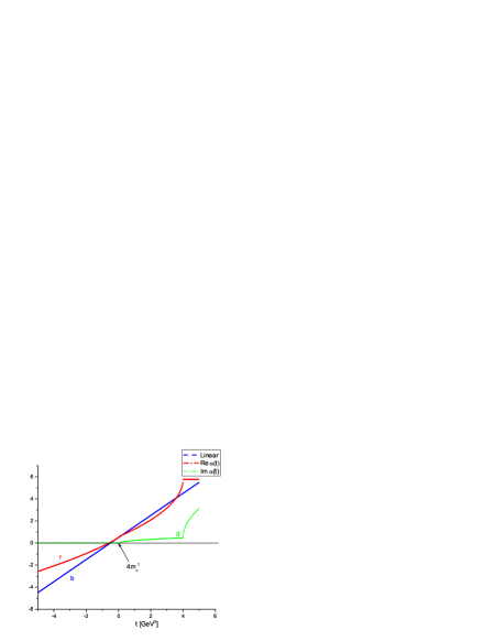
Notice that $M$ does not correspond to any physical resonance; rather it is a parameter to be fitted [23] to the resonances’ spectra, as well as to the scattering data [16]. The construction of Regge trajectories satisfying theoretical constraints on the threshold- and asymptotic behavior, yet compatible with the experimental data, is a highly nontrivial problem. Simple models, like (4), may be helpful as a guide in a semi-quantitative analysis, as in Sec. 6. In a more rigorous approach of Ref. [17] the real and imaginary parts of the trajectories were related by a dispersion relation combined with the unitarity constraints on the threshold behavior and fits to the resonances’ masses and decay widths.

In the limit $|u|,|t|\rightarrow\infty,u/t=const,$ DAMA (1) scales iff its trajectories have logarithmic asymptotics. The simplest trajectory that combines the nearly linear behaviour at small $t$ with a square-root threshold and logarithmic asymptotics is

$$\alpha(t)=\alpha(0)-\gamma\ln\biggl{(}{1+\beta\sqrt{t_{0}-t}\over{1+\beta\sqrt{t_{0}}}}\biggr{)}.$$ (5)

More thresholds (introducing more parameters, however) can be added. Asymptotically, $\alpha(t)\mathop{\simeq}\limits_{t\to\infty}-{\gamma\over 2}\ln(-t).$ The asymptotic (scaling) limit of DAMA can be easily calculated [27] by the saddle-point method, the saddle point, for asymptotically logarithmic trajectories, being located at

$$x_{0}={\alpha(u)\over{\alpha(u)+\alpha(t)}}=1/2.$$

In this limit, the $(ut)$ term of the amplitude (1) goes like [27]

$$D(u,t)\sim(ut)^{-\gamma\ln(2g)/2}.$$ (6)

The power in (6) can be fixed by the quark counting rules [29], by which

$$ln(2g)=2n-1,$$

where n is the number of constituents in a collision. These numbers should not be taken literally (more details can be found in [28]) since they may have more relevance to the leading, vacuum trajectory, while in GPD to be discussed below the main contribution comes from subleading trajectories.

An interesting link between the fixed scattering scattering angle regime of DAMA and composite particle models in the infinite momentum frame [32] was established by M. Schmidt in Ref. [30] .

Figure 2: Diagram for (ut) channel elastic scattering, corresponding to eq. (7)

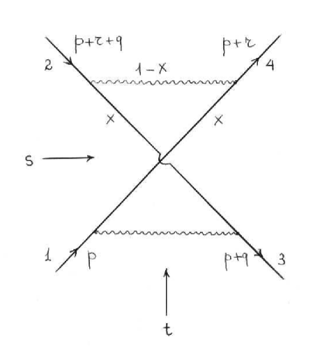
In the model of Gunion, Brodsky and Blankenbecler (GBB) [32], the scattering amplitude corresponding to graph shown in Fig. 2, is given by [32]

$$A(u,t)=\int_{0}^{1}{dx\over{x^{2}(1-x)^{2}}}\int d^{2}k_{\bot}\Delta\psi_{1}(k_{\bot})\psi_{2}(k_{\bot}+$$

$$(1-x)q_{\bot}-xr_{\bot})\psi_{3}(k_{\bot}+(1-x)q_{\bot})\psi_{4}(k_{\bot}+xr_{\bot}),$$ (7)

where the transverse vectors $r_{\bot}$ and $q_{\bot}$ satisfy the conditions $r_{\bot}\cdot q_{\bot}=0,\ \ u=-r_{\bot}^{2},\ \ t=-q_{\bot}^{2},$ in the infinite momentum frame

$$p_{1}=\biggl{(}P+{m^{2}\over{2P}},0,P\biggr{)},$$

$$p_{2}=\biggl{(}P+{{m^{2}+q^{2}_{\bot}}\over{2P}},q_{\bot},P\biggr{)},$$

etc., $P\rightarrow+\infty,$ and $\psi_{i}$ are quark bound state wave functions [32].

The form factor $F(q^{2})$ and the DIS structure function $F_{2}(x)$ in terms of the wave functions $\psi$ are [30]

$$F(q^{2})=\int_{0}^{1}{dx\over{x(1-x)}}\int d^{2}k_{\bot}\psi(k_{\bot})\psi(k_{\bot}+(1-x)q_{\bot})$$

and

$$F_{2}(x)=\int d^{2}k_{\bot}{\psi^{2}(k_{\bot})\over{1-x}}.$$

In the limit $s\approx-u=r^{2}_{\bot}$ and fixed $t=-q^{2}_{\bot}$

$$A(u,t)=\int_{0}^{1}{dx\over{x^{2}(1-x)^{2}}}g(r^{2}_{\bot},x)\int d^{2}k_{\bot}{{\psi(k_{\bot})\psi(k_{\bot}+(1-x)q_{\bot})}\over{x(1-x)}}$$

follows[30], where $g(r^{2}_{\bot},x)\approx\psi(xr_{\bot}),$ while for large $u$ and fixed $t$ one gets [30]

$$A(u,t)\sim\int_{0}^{1}{dx\over{x(1-x)}}g(r^{2}_{\bot})x^{-\alpha(t(1-x))}f(t(1-x)).$$

The parallels between dual (1) and composite models offer at least three lessons:

1) Apart from ”soft” collisions of hadrons (strings) [19], DAMA implicitly contains also the dynamics of hard scattering of the constituents;

2) the variables appearing in combinations like $t(1-x)$, should be used in constructing $t$-dependent parton distributions;

3) Regge trajectories are non-linear, complex functions with well-defined constrains.

3 Form factors; analyticity and unitarity

In this section we present general properties of the form factors with emphasis on their analytic properties and connection with Regge trajectories, to be utilized in subsequent sections.

There are various choices for the nucleon electromognetic form factors (ff), such as the Dirac and Pauli ff, $F_{1}^{p}(t),\ \ F_{1}^{n}(t)$ and $F_{2}^{p}(t),\ \ F_{2}^{n}(t),$ the Sachs electric and magnetic ff, $F_{E}^{p}(t),\ \ F_{E}^{n}(t)$ and $F_{M}^{p}(t),\ \ F_{M}^{n}(t),$ or isoscalar and isovector electric and magnetic ff, $F_{E}^{s}(t),\ \ F_{E}^{v}(t)$ and $F_{M}^{s}(t),\ \ F_{M}^{v}(t)$, where $t=-Q^{2}$ is the squared momentum transfer of the virtual photon [34].

The Dirac and Pauli form factors are obtained from a decomposition of the matrix element of the electromagnetic (e.m.) current in linearly independent covariants made of four-momenta, $\gamma$ matrices and Dirac bispinors as follows

$$<N|J_{\mu}^{e.m.}|N>=e\bar{u}(p^{\prime})[\gamma_{\mu}F_{1}^{N}(t)+{i\over{2m}}\sigma_{\mu\nu}(p^{\prime}-p)_{\nu}F_{2}^{N}(t)]u(p),$$

where $m$ is the nucleon mass. Electric and magnetic ff, on the other hand, are suitable in extracting them from the experiment:

$$\begin{array}[]{l}\displaystyle{{d\sigma^{lab}(e^{-}N\rightarrow e^{-}N)}\over{d\Omega}}=\\ \displaystyle={{\alpha_{e.m.}^{2}\cos^{2}(\theta/2)}\over{4E^{2}\sin^{4}(\theta/2)}}{1\over{1+\bigl{(}{{2E}\over{m}}\bigr{)}\sin^{2}(\theta/2)}}\Biggl{(}{{G_{E}^{2}-{t\over{4m^{2}}}G^{2}_{M}}\over{1-{t\over{4m^{2}}}}}-2{t\over{4m^{2}}}G^{2}_{M}\tan^{2}(\theta/2)\Biggr{)},\end{array}$$

where $\alpha_{e.m.}=1/137,\ \ E$ is the incident electron energy, and

$$\sigma_{tot}^{e.m.}(e^{+}e^{-}\rightarrow N\bar{N})={{4\pi\alpha_{e.m.}^{2}\beta}\over{3t}}[|G_{m}(t)|^{2}+{{2m^{2}}\over t}|G_{E}(t)|^{2}],\ \ \beta=\sqrt{1-{{4m^{2}}\over t}},$$

or

$$\sigma_{tot}^{e.m.}(p\bar{p}\rightarrow e^{+}e^{-})={{4\pi\alpha_{e.m.}^{2}\over{3p_{c.m.}}\sqrt{t}}}[|G_{M}(t)|^{2}+{2m^{2}\over t}|G_{E}(t)|^{2}],$$

where $p_{c.m.}$ is the proton momentum in the c.m. system.

The four independent sets of form factors are related by

$$G_{E}^{p}(t)=G_{E}^{s}(t)+G_{E}^{v}(t)=F_{1}^{p}(t)+\tau^{p}F_{2}^{p}(t)=[F_{1}^{s}(t)+F_{1}^{v}(t)]+\tau^{p}[F_{2}^{s}(t)+F_{2}^{v}(t)],$$ (8)

$$G_{M}^{p}(t)=G_{M}^{v}(t)+G_{M}^{v}(t)=F_{1}^{p}(t)+F_{2}^{p}(t)=[F_{1}^{s}(t)+F_{1}^{v}(t)]+[F_{2}^{s}(t)+F_{2}^{v}(t)],$$ (9)

$$G_{E}^{n}(t)=G_{E}^{s}(t)-G_{E}^{v}(t)=F_{1}^{n}(t)+\tau^{n}F_{2}^{n}(t)=[F_{1}^{s}(t)-F_{1}^{v}(t)]+\tau^{n}[F_{2}^{s}(t)-F_{2}^{v}(t)],$$ (10)

$$G_{M}^{n}(t)=G_{M}^{s}(t)-G_{M}^{v}(t)=F_{1}^{n}(t)+F_{2}^{n}(t)=[F_{1}^{s}(t)-F_{1}^{v}(t)]+[F_{2}^{s}(t)-F_{2}^{v}(t)],$$ (11)

where $\tau^{p(n)}={t\over{4m_{p(n)}^{2}}}.$ They satisfy the normalization conditions

$$G_{E}^{p}(0)=1;\ G_{M}^{p}(0)=1+\mu_{p};\ G^{n}_{R}(0)=0;G^{n}_{M}(0)=\mu_{n};$$

$$G_{E}^{s}(0)=G_{E}^{v}(0)={1\over 2};\ G_{M}^{s}(0)={1\over 2}(1+\mu_{p}+\mu_{n});\ G_{M}^{v}(0)={1\over 2}(1+\mu_{p}-\mu_{n});$$

$$F_{1}^{p}(0)=1;\ F_{2}^{p}(0)=\mu_{p};\ F_{1}^{n}(0);\ F_{2}^{n}(0)=\mu_{n};$$

$$F_{1}^{s}(0)=F_{1}^{v}(0)={1\over 2};\ F_{2}^{s}(0)={1\over 2}(\mu_{p}+\mu_{n});\ F_{2}^{v}(0)=(\mu_{p}-\mu_{n}),$$

where $\mu_{p}$ and $\mu_{n}$ are the proton and neutron anomalous magnetic moments, respectively.

A basic ingredient of the existing models of form factors [34] is the dominance of the $\rho$ meson pole, resulting e.g. for the isovector meson form factor to the expression

$$G_{v}(t)={g_{\rho}^{2}\over{1-t/m_{\rho}^{2}}},$$

where $g_{\rho}$ is a constant proportional to the product of $\gamma\rho$ and $\gamma NN$ couplings. The next step is to include [35] other vector mesons, as well as their excitations, such as the isovector: $\rho(770),\ \rho^{\prime}(1450),\ \rho^{\prime\prime}(1700)$ and isoscalar resonances $\omega(782),\ \omega^{\prime}1420),\ \omega^{\prime\prime}(1600),\ \phi(1020),\ \phi(1680)$ found in the Review of Particle Physics.

The use of the trajectories implies a single ”dual” variable instead of the parameters of individual resonances. The approach of Ref. [17] combines the concept of Regge trajectories with analyticity, unitarity and resonance data analysis. An economic way to account for the exciting states is to use Regge trajectories, advocated in the present paper and bringing us close to dual models. Soon after the discovery of Veneziano’s dual model [19], attempts were made [36] to apply it to form factors. Assuming an infinity number of neutral vector mesons with the sequence of squared masses $m^{2}(n)=m_{0}^{2}+nm_{1}^{2},\ n=0,1,...$ the following expression proton magnetic form factor was derived [36]

$${G_{M_{p}}(t)\over{\mu_{p}}}={{\Gamma[1-\alpha(t)]\Gamma[c-\alpha(0)]}\over{\Gamma[1-\alpha(0)]\Gamma[c-\alpha(t)]}},$$

where $\alpha(t)$ is the $\rho$ trajectory and $c=3.27.$

Unitarity constrains the threshold behavior of the Regge trajectories [22] (see also [17] and references therein) as well as that of the form factors [39]

$$\Im F_{\pi}(t)\mathop{\sim}\limits_{t\to t_{0}}(t-t_{0})^{1-\Re\alpha(t_{0})}\Im\alpha(t)\sim(t-t_{0})^{3/2},$$

where $t_{0}=4\pi^{2}_{\pi}.$ Any finite width of the resonances requires an imaginary part to be added, as for example was done in Ref. [37]

$${G_{M_{p}}(t)\over{\mu_{p}}}=\sum_{i=\rho,\omega,\phi}a_{i}\Bigl{(}t-m_{i}^{2}+\gamma_{i}\sqrt{b_{i}^{2}-t}\Bigr{)}^{-1},$$

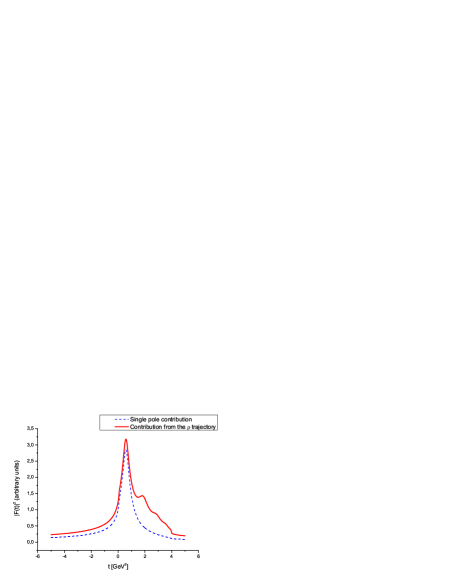
where $\gamma_{i}$ are resonances’ widths and the fitted values of the parameters $b_{i}$ are: $b_{\rho}=0.28$ GeV, $b_{\omega}=0.42$ GeV, $b_{\phi}=0.99$ GeV. This approach is close in spirit to that based on dual analytic model, introduced in the previous section, and illustrated in Figs. 1, showing the calculated modulus of the form factor resulting from a single $\rho$ pole contribution (dotted line) and from a sequence of poles generated by trajectory (4)

$${G_{M_{p}}\over{\mu_{p}}}=\left|\sum_{j=1}^{\infty}{(0.5)^{j}\over{(j-\alpha(\rho))}}\right|.$$ (12)

This sum is similr to the pole decomposition of the dual amplitude, namely it is a sum of ”reggeized” implied by duality) Breit-Wigner resonances (cf. (2)). The upper limit of summation includes the highest resonance lying on the $\rho$ trajectory (4), however the large-$|t|$ behaviour of the form factor, Fig. 3, is not affected by higher spin values (here, $j>5$, up to infinity), from where the real part of the trajectory does not contribute any more. The inclusion of a large (infinite) number of poles appearing on the second sheet is important in dual models [18]. The non-appearance of higher resonances and the transition to a smooth continuum can result either from an upper bound on the real part of the trajectory, as is DAMA [18], or from the rapid rise of its imaginary part, making the resonances unobservable.

Similarly to the Veneziano model, form factors were derived [38] from DAMA (1):

$$F(t)_{\pi}=\int_{0}^{1}dxx^{-\alpha(t(1-x))}(1-x)^{-1+n},$$ (13)

where $n$ is an integer providing the correct (according to quark counting rules) large-$|t|$ behavior of the form factor.

Calculations of form factors from GPD, Sec. 4-6, are more involved and less predictable, especially in the case of complex Regge trajectories.

4 Generalized parton distributions and form factors

Form factors are related to generalized parton distributions (GPD) by the standard sum rules [2, 3]

$$F_{1}^{q}(t)=\int_{-1}^{1}dxH^{q}(x,\xi,t),$$

$$F_{1}^{q}(t)=\int_{-1}^{1}dxH^{q}(x,\xi,t).$$

The integration region can be reduced to positive values of $x,~{}0<x<1$ by the following combination of non-forward parton densities [12, 14]

$${\cal H}^{q}(x,t)=H^{q}(x,0,t)+H^{q}(-x,0,t),$$

$${\cal E}^{q}(x,t)=E^{q}(x,0,t)+E^{q}(-x,0,t),$$

providing

$$F^{q}_{1}(t)=\int_{0}^{1}dx{\cal H}^{q}(x,t),$$ (14)

$$F^{q}_{2}(t)=\int_{0}^{1}dx{\cal E}^{q}(x,t).$$ (15)

The proton and neutron Dirac form factor are defined as

$$F_{1}^{p}(t)=e_{u}F_{1}^{u}(t)+e_{d}F_{1}^{d}(t),$$

$$F_{1}^{n}(t)=e_{u}F_{1}^{d}(t)+e_{d}F_{1}^{u}(t),$$

where $e_{u}=2/3$ and $e_{d}=-1/3$ are the relevant quark electric charges.

In the limit $t\rightarrow 0$ the functions $H^{q}(x,t)$ reduce to usual valon quark densities in the proton:

$${\cal\ H}^{u}(x,t=0)=u_{v}(x),\ \ \ {\cal H}^{d}(x,t=0)=d_{v}(x)$$

with the integrals

$$\int_{0}^{1}u_{v}(x)dx=2,\ \ \ \int_{0}^{1}d_{v}(x)dx=1$$

normalized to the number of $u$ and $d$ valence quarks in the proton.

Contrary to ${\cal H},$ the ”magnetic” densities ${\cal E}^{q}(x,t=0)\equiv{\cal E}^{q}(x)$ cannot be directly expressed in term of the known parton distributions, however their normalization integrals

$$\int_{0}^{1}{\cal E}^{q}(x)dx\equiv k_{q}$$

are constrained by the requirement that the values $F_{2}^{p}(t=0)$ and $F_{2}^{n}(t=0)$ are equal to the magnetic moments of the proton and neutron, whence $k_{u}=2k_{p}+k_{n}\approx 1.673$ and $k_{u}=k_{p}+2k_{n}\approx-2.033$ follows [14]. Explicit parameterizations for the forward and non-forward structure functions as will be presented in the next section.

The Fourier-Bessel integral

$$q(x,b)={1\over 2\pi}\int_{0}^{\infty}d\sqrt{-t}J_{0}(b\sqrt{-t}){\cal H}(x,t)$$ (16)

provides a mixed representation of longitudinal momentum and transverse position in the infinite-momentum frame [4, 5].

5 Modelling non-forward parton distributions;
connection with Regge-dual models

The simplest model for the proton non-forward parton density is a factorized form

$${\cal H}(x,t)=q_{v}(x)F_{1}(t),$$ (17)

here $q_{v}(x)$ is the parton density and $F_{1}(t)$ is the proton form factor. It trivially reproduces $F_{1}^{p}(t)$ and $q_{v}(x)$ in the forward limit, but it conflicts both with Regge (R) behavior

$${\cal H}_{R}(x,t)\sim x^{-\alpha(t)},$$ (18)

valid at small $x,$ and with the light-cone formalism, suggesting a Gaussian (G) parametrization for non-forward parton densities [40, 12]

$${\cal H}_{G}^{q}(x,t)=q_{v}(x)e^{-(1-x)t/4x\lambda^{2}},$$

where the scale $\lambda^{2}$ characterizes the average transverse momentum of the valence quarks in the nucleon. To satisfy the Drell-Yan-West (DYW) relation [41, 42] between the $x\to 1$ behavior of the structure functions and the $t-$dependence of the elastic form factors the above expression should be modified e.g. as [14]

$${\cal H}^{q}(x,t)=q_{v}(x)x^{-\alpha^{\prime}(1-x)t},$$ (19)

where $\alpha^{\prime}$ is the slope of a Regge trajectory (other modifications of the parton distributions as well as their relation to the light-cone wave function of a composite system are discussed in [4, 5]). Noticing the similarity between this expression and the relevant factor in the integrand of (1), we suggest the following parametrization for the $t-$dependent GPD:

$${\cal H}_{G}^{q}(x,t)=q_{v}(x)(x/g_{0})^{-\tilde{\alpha}(t)(1-x)t}=(x/g_{0})^{-\alpha(t)(1-x)}f(x),$$ (20)

where $\tilde{\alpha}(t)$ is the $t-$dependent part of the Regge trajectory, $g_{0}>1$ ($x_{0}$ in Ref. [15]) is a parameter defined in Sec. 2 and $f(x)$ is the large-$x$ factor of the parton distribution (see below). For linear trajectories and $g_{0}=1,$ eq. (20) reduces to (19).

Regge behavior $\sim x^{-\alpha(0)}$ of DIS structure functions and relevant parton distributions at small $x$ is well established for small and moderate virtualities $Q^{2};$ at higher $Q^{2}$ it is replaced by QCD evolution (see e.g. [43] and references therein). The values of the ”Regge-intercepts” in the parton distributions may depend on the flavor of the relevant quark. For example, in the global fits of MRST2002 [44]:

$$u_{v}(x)=0.262x^{-0.69}(1-x)^{3.50}(1+3.83x^{0.5}+37.65x),$$ (21)

$$d_{v}(x)=0.061x^{-0.65}(1-x)^{4.03}(1+49.65x^{0.5}+8.65x),$$ (22)

implying $\alpha(0)=0.69$ in the $u$-quark distribution and $0.65$ in the $d$-quark distribution, which means slightly different trajectories exchanged in the $t$-channel of the (fictive) $\bar{u}p$ and $\bar{d}p$ scattering amplitude, once the GPD is associated with the imaginary part of the $u-$ channel quark-proton scattering amplitude. We use these expressions in our calculations below.

The ”magnetic” densities ${\cal E}^{q}(x,t)$ enter in $F_{2}(t)$ and contain new information about the nucleon structure, however they cannot be directly expressed in terms of any known parton distribution. Following [14], we write them in the form ${\cal E}^{q}(x,t)={\cal E}^{q}(x)x^{-(1-x)\alpha_{E}^{\prime}t},\ \alpha_{E}^{\prime}=1.158GeV^{-2},$ similar to ${\cal H}^{q}(x,t)$ but with an extra large-$x$ factor, i.e.

$${\cal E}^{u}(x)={k_{u}\over{N_{u}}}(1-x)^{\eta_{u}}u_{v}(x)$$ (23)

and

$${\cal E}^{d}(x)={k_{d}\over{N_{d}}}(1-x)^{\eta_{d}}d_{v}(x),$$ (24)

with $\eta_{u}=1.52$ and $\eta_{d}=0.31$ fitted [14] to the data. The remaining constants are fixed by normalization:

$$N_{u}=\int_{0}^{1}dx(1-x)^{1.52}u(x)=1.53;$$

$$N_{d}=\int_{0}^{1}dx(1-x)^{0.31}d(x)=0.82,$$

whence $k_{u}\approx 1.673,\ k_{d}\approx-2.033.$

6 Numerical estimates

Below we illustrate how the nonlinearity (complexity) of the trajectories and the introduction of $g_{0}>1$ affect the behavior of the calculated form factors and quark distributions as functions of the impact parameter $b$ and of the Bjorken variable $x.$

Figure 3: Left panel: Proton magnetic form factor relative to the dipole form factor (left upper panel) and the ratio of the magnetic to electric form factors (left lower panel). The black thin curves correspond to the linear trajectory of Ref. [14], the red (r) curve to the nonlinear trajectory (24) with $g_{0}=1,$ and the blue (b) curve to the same nonlinear trajectory but with $g=1.05.$ The data for the proton magnetic form factor $G_{M}^{p}$ are from [46] (open squares), [47] (open circles), [48] (solid stars), [49] (open stars), [50] (solid circles), [51] (solid squares), and those for the ratio $G^{p}_{E}/G^{p}_{M}$ are from [52] (solid circles), [53] (open triangles) and [54] (solid triangles). Right panel: Ratio of the neutron magnetic form factor to the dipole form factor (right upper panel) and neutron electric form factor (right lower panel) with curve conventions as on the left panel. The data for the neutron magnetic form factor $G_{M}^{n}$ are from [55] (open circles), [56] (solid circles), [57] (open triangles), [58] (solid triangles), [59] (solid squares) and [60] (solid squares). The data for the neutron electric form factor are from MAMI [61] (triangles), NIKHEF [62] (solid squares) and JLab [63] (solid circles) and [64] (open squares).

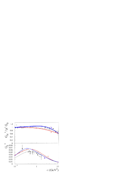
We first explore the effects coming from non-linear Regge trajectories by calculating several observable form factors and their ratios using the expressions for the $t-$dependent GPD, eq. (20). As a reference frame, we use fits from the paper [14] nicely reproducing the data. In that paper linear trajectories with the slopes $\alpha_{1}^{\prime}=1.098$ GeV² in ${\cal H}(x,t)$ and $\alpha_{2}^{\prime}=1.158$ GeV² in ${\cal E}(x,t)$ were used. The relevant intercepts come from the parton distributions (21), (22), and they are equal to $0.69$ and $0.65$ in the $u$ quark and $d$ quark distributions, respectively [44]. With these parameters (and $g_{0}=0,$ matching the model of ref. [14]) one reproduces the results of Ref. [14], some of them shown in Fig.3 in thin black line.

Figure 4: Impact-parameter distribution of the $u$ quark matter at $x=0.1$ (left panel), $x=0.5$ (middle) and $x=0.7$ (right panel). The curves on the left panel correspond (from the top) to calculations with: $\tilde{\alpha}(t)=1.098t$ (red, solid line); eq. (4) (green, dotted line) and the logarithmic trajectory eq. (5) with $\gamma=0.3,\ \beta=0.366$ and $t_{0}=4m_{\pi}^{2}$ (blue, dotted line). Curves on the middle and right panel correspond to calculations with eq. (4) (green dotted line) and the above linear trajectory (red solid line). Those with the logarithmic trajectory (5) for $x>0.3$ go off the common trend.

Next we explore the effects coming from the nonlinearity of the Regge trajectories, as well as from $g_{0}>1,$ both introduced in Sec.2. By keeping the less known ${\cal E}^{q}(x,t)$ intact we vary the trajectory in ${\cal H}^{u}(x,t)$ and the value of $g_{0}.$ The effect proves to be very large. For example, even a minor (with respect e.g. to (4)) deviation from the linear trajectory,

$$\tilde{\alpha}(t)=1.026t-0.02(\sqrt{4m_{\pi}^{2}-t}-2m_{\pi}),$$ (25)

with the forward slope $\alpha^{\prime}\approx 1.098GeV^{-2}$ matching the linear trajectory fitted in [14] to the data, gives a sizable effect, augmenting e.g. the ratio $G_{M}^{p}/\mu^{p}G_{D}$, as seen in Fig.3 (red line).

Figure 5: Longitudinal momentum distribution of the $u$ quark matter calculated with a linear trajectory $\tilde{\alpha}(t)=1.098t$ (left panel) and eq. (4) (right panel). The curves (from the top) correspond to: [$t=-0.7GeV^{2},g_{0}=1$] (red line), $[t=-0.9GeV^{2},g_{0}=2]$ (blue line), $[t=-0.7GeV^{2},g_{0}=5]$ (green line), $[t=-3GeV^{2},g_{0}=1]$ (pink line).

The effect from $g_{0}>1,$ combined with the nonlinear trajectory, is shown in Fig. 3 (blue line). In general, it compensates the rise due to the nonlinearity of the trajectory, although the interplay of these two effects is much more complicated. The use of analytic trajectories and/or $g_{0}>1$ in ${\cal E}^{q}(x,t)$ will make the situation much more complicated but, but at the same time, interesting. The use of a ”realistic” trajectory like eq. (4) changes the behavior of the observables dramatically, requiring a complete rearrangement of the model or, at least, of its parameters.

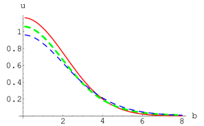
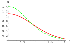
Fig. 4 shows the $u$ quark impact parameter distribution calculated from eqs. (16), (20) at three fixed values of $x=0.1,\ 0.5$ and $0.7$ and for three representative trajectories: linear, $\tilde{\alpha}(t)=1.098t$ (red (r) curves), ”square root”, eq. (4) (green (g) curves) and logarithmic, eq. (5) with $\gamma=3,\ \beta=0366GeV^{-2}$ and $t_{0}=4m_{\pi}^{2}$ (blue (b) curves). The calculated distributions depend dramatically on the form of the trajectories, especially near the endpoints $x=0$ and $1$.

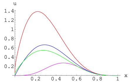
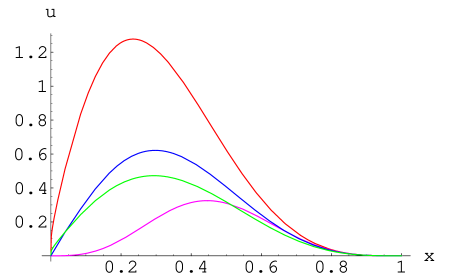
The role of the parameter $g_{0},$ combined with the variation of the trajectories, can be seen also in Fig. 5, where the $u$ quark distribution is plotted against $x$ for several fixed values of $t$ and of $g_{0}$ and two typical trajectories: a linear one, $\tilde{\alpha}(t)=1.098t,$ and (4). Here the dependence on the form of the trajectories is less pronounced then in Fig. 4, where integration in $t$ is involved.

Given the available freedom in the choice of the trajectories, the present calculations can serve only as an indication of the existing trends, rather then fits or predictions to the data.

7 Conclusions and outlook

With this paper we wish to emphasize the important role of the analytic properties of the strong interaction theory, manifest here in the form of the Regge trajectories. The wide-spread prejudice that the trajectories are linear has different sources: 1) the masses of the resonances lie on approximately linear trajectories; 2) the Veneziano and string models [19] provide a theoretical basis in favor of this behavior; 3) relevant calculations are simple. On the other hand, the theory demands that the trajectories be analytic functions of their arguments with threshold singularities imposed by unitarity, and that the asymptotic behavior be compatible with the polynomial boundedness of the amplitude. Trajectories satisfying these constraints and fitting the data both for positive (particles spectra) and negative (scattering data) values of their arguments are known from the literature (see, e.g., [16, 17]). In this paper we show that they affect considerably the calculated GPD and their moments. More work is needed to specify and quantify the role of various (parent and daughter) subleading trajectories (of poles and cuts).

Another message of this paper is that, in a certain kinematical region, the integrand of the dual amplitude with Mandelstam analyticity (DAMA) (1) can be identified with a generalized parton distribution (GPD), the integration variable being associated with the parton longitudinal momentum, as suggested in [31]. For fixed $Q^{2}$ and $s,$ the integrand of DAMA (1) (a GPD?) has the form

$$(x/g_{0})^{-\tilde{\alpha}(t(1-x))-n}((1-x)/g_{0})^{m},$$ (26)

where $g_{0}>1,$ and $n$ and $m$ are reaction-dependent constants. The first factor in (26) is the small-$x$ Regge-behaved term, while the second one is the familiar large-$x$ term. An immediate observation is the similarity between the moments of the GPD (form factors), eq. (14) and expression (13), derived from DAMA. I wonder if this could mean a bootstrap relation between the antiquark-hadron scattering amplitude (GPD) and the hadron-hadron amplitude resulting from integration (1) of a GPD ? The appearance of $x$ in the exponents of the (modified) structure functions, (or parton distributions) may have interesting consequences by itself – both for theory and phenomenology. In any case, a better understanding of the physical meaning of the variables appearing in GPD, especially with non-zero skewedness, $\xi\neq 0,$ is needed.

The approach in this paper combines elements of the analytic $S-$ matrix theory, namely Regge poles and duality, known to be efficient for ”soft” collisions at large distances, with the small-distance partonic picture. The interface and merge of these seemingly orthogonal approaches may bring new ideas about the transition form perturbative to non-perturbative physics. Much of this information is encoded in the form of the complex Regge trajectories. Recently, explicit models for deeply virtual Compton scattering amplitudes (DVCS) appeared in the literature [66]. Their imaginary part can provide additional information about GPD.

In a perspective one can think of extending the asymptotic Regge pole model to the low-energy resonance region by incorporating a dual amplitude, e.g., DAMA. The crossing-symmetric properties of dual amplitudes will make possible the inclusion of the $t>0$ region in DVCS and resulting GPD. It may also help to connect the high-energy (Regge) region with the low-energy (resonance) domain, where new data from JLab is expected.

References

- [1] D. Müller, D. Robaschik, G. Geyer, F.M. Dittes and J. Horejsi, Fortschr. Phys. 42 (1994) 101.
- [2] A.V. Radyushkin, Phys. Rev. D 56(1997) 5524.
- [3] X. Ji, J. Phys. G 24 (1998) 1181.
- [4] M. Burkardt, Phys. Rev. D 62 (2000) 071503 [Erratum-ibid. D 66 (2002) 119903] [arXiv:hep-ph/0005108].
- [5] M. Burkardt, Int. J. Mod. Phys. A 18 (2003) 173 [arXiv: hep-ph/0207047].
- [6] M. Diehl, Eur. Phys. J. C 25 (2002) 223 [Erratum-ibid. C 31 (2003) 277] [arXiv:hep-ph/0205208].
- [7] John P. Ralston and Bernard Pire, Femto-Photography of Protons in Nuclei with Deeply Virtual Compton Scattering [arXiv:hep-ph/0110075]; A.V. Belitsky, D.Muller, Nucleon Hologram with Exclusive Leptoproduction [arXiv:hep-ph/0206306]; B. Pire and L. Szymanowski, Hard Exclusive Reactions and Hadron Structure [arXiv:hep-ph/0607132].
- [8] A.V. Belitsky, X.D. Ji and F. Yuan, Phys. Rev. D 69 (2004) 074014 [arXiv:hep-ph/0307383].
- [9] A.V. Radyushkin, in the Boris Ioffe Festschrift ”At the Frontiers of Particle Physics / Handbook of QCD”, edited by M. Shifman (World Scientific, Singapore, 2001); M. Goeke, M.V. Polyakov and V. Vanderhaegen, Progr. Part. Nucl. Phys. 47 (2001) 401 [arXiv:hep-ph/0106012]; M. Diehl, Phys. Rept. 388 (2003) 41 [arXiv:hep-ph/0307382].
- [10] R. Fiore, L.L. Jenkovszky, V.K. Magas, In Proc. of Diffraction2004, Nuclear Phys. B (Proc. Suppliment) 146 (2005) 146; In Proc. of the XXXIV-th ISMD, Acta Phys. Pol. 36 (2005) 743; L. Jenkovszky, V. Magas, A. Vall, Physics of Particles and Nuclei 16 Suppl. 2 (2005) S152.
- [11] M. Burkardt, Phys. Lett. B595 (2004) 245 [arXiv:hep-ph/0401159].
- [12] A.V. Radyushkin, Phys. Rev. D 58 (1998) 114008 [arXiv9803316].
- [13] S.J. Brodsky et al., Nucl. Phys. B 596 (2001) 99.
- [14] M. Guidal, M.V. Polyakov, A.V. Radyushkin, and M. Vanderhaeghen, Phys. Rev. D 72 (2005) 054013 [arXiv:hep-ph/0410251].
- [15] M. Diehl, T. Feldmann, R. Jakob and P. Kroll, Eur. Phys. J. C 39 (2005) 1. [arXiv:hep-ph/0408173.
- [16] L.L. Jenkovszky, A.N. Shelkovenko, B.V. Struminsky, Z. Phys. C36 (1987) 1200; P. Desgrolard, M. Giffon, E.S. Martynov, and E. Predazzi, Eur. Phys. J. C18 (2001) 555.
- [17] R. Fiore, L.L. Jenkovszky, V.K. Magas, F. Paccanoni, A. Papa, Eur. Phys. J. A 10 (2001) 217; Nucl. Phys. B (Proc. Suppl.) 99 (2001) 68.
- [18] See: A.I Bugrij, G. Cohen-Tannoudji, L.L.Jenkovszky, N.A. Kobylinsky, Fortschr. Phys, 21 (1973) 427 and earlier references therein.
- [19] G. Veneziano, Nuovo Cim. 57A (1968) 199; Phys. Rep. 9 (1974) 199; for an up-do-date review see: W. Melnitchouk, R. Ent, and C.E. Keppel, Phys. Rep. 406 (2005) 127 [arXiv:hep-ph/0501217].
- [20] A. Degasperis and E. Predazzi, Nuovo Cim. A65 (1970) 764.
- [21] A.A. Trushevsky, Ukrainian Phys. J. 127 (1962) 357.
- [22] A.O. Barut and D.E. Zwanziger, Phys. Rev. 127 (1962) 974.
- [23] A.I. Bugrij and N.A. Kobylinsky, Ann. Phys. (DDR) 32 (1975) 297.
- [24] A.I. Bugrij, private communication.
- [25] M.M. Brisudova, L. Burakovsky, T.Goldman, Phys. Rev. D 61 (2000) 054013.
- [26] G. Cohen-Tannoudji et al. Lettere al Lettere Nuovo Cim., 5 (1072) 957; A. Anselm and V. Gribov, Phys. Letters 40B (1972) 487.
- [27] L.L. Jenkovszky, Z.E. Chikovani, Yad. Fizika 30 (1979) 531; A.I. Bugrij, Z.E. Chikovani, L.L. Jenkovszky, C4 (1980) 45; R. Fiore, L.Jenkovszky, V. Magas and F. Paccanoni, Phys. Rev. D60 (1999) 116003.
- [28] László L. Jenkovszky, Nucl. Phys. B (Proc. Suppl.) 12 (1990) 317.
- [29] V.A. Matveev, R.M. Muradyan and A.N. Tavkhelidze, Lettere Nuovo Cim, 7 (1973) 719; S. Brodsky, G. Farrar, Phys. Rev. Lett. 31 (1973) 1153.
- [30] M.G. Schmidt, Phys. Letters, 43B (1973).
- [31] R. Fiore and L. Jenkovszky, In: Elastic and Diffractive Scattering, Proc. of the VIII-th Blois conf., A. Prokudin and V. Petrov eds., World Scientific, 2000, p. 261.
- [32] J.F. Gunion, S.J. Brodsky, and R. Blankenbecler, Phys. Letters 39B (1972) 649.
- [33] D.D. Coon, J.F. Gunion, Tran Thanh Van, R.Blankenbecler, Phenomenlogy of High Momentum Transfer Elastic Processes, SLAC-PUB-1483, Phys. Rev. D 18 (1978) 1451.
- [34] See, e.g.: M. Gourdin, Physics Reports, 11 (1974) 30; N. Zovko, Fortschritte der Physik, 23 (1975) 185; A.I. Akhiezer and M.P. Rekalo, Electrodynamics of Hadrons, Naukova Dumka, Kiev, 1977 (in Russian).
- [35] Stanislav Dubnicka, Anna Dubnickova, and Peter Weisenpacher, J. Phys. G29 (2003) 405 [arXiv:hep-ph/0208051].
- [36] P.H. Frampton, Phys. Rev. 186 (186) 1419; P. Di Vecchia, F. Drago, Lett. Nuovo Cim. 1(1969) 917; H. Sura, Phys. Rev. Lett. 23 (1969) 551; Y. Oyanagi, Progr. Theor. Phys. 42 (1969).
- [37] V. Wataghin, Nuovo Cim., 54A (1958) 805; ibid: 54A (1968) 840.
- [38] F.B. Prognimak, Preperint ITP-76-44E, Kiev, 1976.
- [39] W. Frazer and J. Fulco, Phys. Rev. 119 (1960) 1603; ibid 119 (1960) 1420.
- [40] V. Barone, M. Genovese, N.N. Nikolaev, E. Predazzi and B.G. Zakharov, Z.Phys. C 58 (1993) 541.
- [41] S.D. Drell and T.M. Yan, Phys. Rev. Lett. 24 (1970) 181.
- [42] G.B. West, Phys. Rev. Lett. 24 (1970) 1206.
- [43] P. Desgrolard, L.L. Jenkovszky, F. Paccanoni, Eur. Phys. J. C 7 (1999) 263; L. Csernai et al. Eur. Phys. J. C 24 (2002) 205.
- [44] A.D. Martin, R.G. Roberts, W.J. Stirtling, and R.S. Thorne, Phys. Lett. B 531 (2002) 216 [arXiv: hep-ph/0201127].
- [45] A. Bugrij et al., Letter Nuovo Cim. 6 (1973) 577.
- [46] T. Janssens at al., Phys. Rev. B 142 (1966) 922.
- [47] J. Litt at al., Phys. Lett. B 31 (1970) 40.
- [48] Ch. Berger at al., Phys. Lett. B 35 (1971) 87.
- [49] W. Bartel at al., Nucl. Phys. B 58 (1973) 429.
- [50] L. Andivahis at al., Phys. Rev. D 50 (1994) 5491.
- [51] A.F. Still at al., Phys. Rev. D 48 (1993) 29.
- [52] M.K. Jones at al., [Jefferson Lab. Hall A Collab.], Phys. Ref. Lett. 84 (2000) 1398 [arXiv:nucl-ex/9910005].
- [53] O. Gajou at al., Phys. Rev. C 64 (2001) 038202.
- [54] O. Gajou at al., [Jefferson Lab. Hall A Collab.], Phys. Rev. Lett. 88 (2002) 092301 [arXiv:nucl-ex/0111010].
- [55] P. Markovitz at al., Phys. Rev. C 48 (1993) 5.
- [56] W. Xu at al., Phys. Rev. Lett. 85 (2000) [arXiv:nucl-ex/0008003].
- [57] H. Anklin at al., Phys. Lett. B 428 (1998) 248.
- [58] G. Kubon at al., Phys. Lett. B 524 (2002) 26 [arXiv:nucl-ex/0107016].
- [59] A. Lung at al., Phys. Rev. Lett. 70 (1993) 718.
- [60] S. Rock at al., Phys. Rev. Lett. 49 (1982) 1139.
- [61] C. Herberg at al., Eur. Phys. J. A. 5 (1999) 131; M. Ostrick, at al., Phys. Rev. Lett. 83 (1999) 276; J. Becker at al., Eur. Phys. J. A 6 (1999) 320; D. Rohe at al., Phys. Rev. Lett. 83 (1999) 4257.
- [62] I. Passchier at al., Phys. Rev. Lett. 82 (1999) 4988 [arXiv:nucl-ex/9907012].
- [63] H. Zhu at al., [E93026 Collab.] 87 (2003) 122002 [arXiv:nucl-ex/0105001]; G. Warren at al., [JLab E93-026 Collab.], Phys. Rev. Lett. 92 (2004) 042301[arXiv:nucl-ex/0308021]; R. Madey at al., Phys. Rev. Lett. 91 (20003) 122002 [arXiv:nucl-ex/0308007];
- [64] R. Schiavilla and I. Sick, Phys. Rev. C 64 (2001) 041002 [arXiv:nucl-ex/0107004].
- [65] Anatoly Radyushkin, QCD Sum Rules and Models for Generalized Parton Distributions, Dedicated to Klaus Goeke on his 60th birthdate [arXiv:/hep-ph/0410153].
- [66] A.P. Szczepaniak and J.T. Longedran, Exclusive Eectroproduction and Quark Structure of the Nucleon [arXiv:hep-ph/0604266]; Dieter Muller, Pomeron Dominance in Deeply Virtual Compton Scattering and Femto Holographic Image of Proton [arXiv:hep-ph/0605013]; M. Capua, F. Fazio, R. Fiore, L. Jenkovszky and F. Paccanoni, A Deeply Virtual Compton Scattering Amplitude [arXiv:hep-ph/0605319].