Determination of the Atmospheric Neutrino Fluxes from Atmospheric Neutrino Data
Abstract:
The precise knowledge of the atmospheric neutrino fluxes is a key ingredient in the interpretation of the results from any atmospheric neutrino experiment. In the standard data analysis, these fluxes are theoretical inputs obtained from sophisticated numerical calculations based on the convolution of the primary cosmic ray spectrum with the expected yield of neutrinos per incident cosmic ray. In this work we present an alternative approach to the determination of the atmospheric neutrino fluxes based on the direct extraction from the experimental data on neutrino event rates. The extraction is achieved by means of a combination of artificial neural networks as interpolants and Monte Carlo methods for faithful error estimation.
UB-ECM-PF-06/16
YITP-SB-06-31
IC/2006/064
1 Introduction and Motivation
One of the most important breakthroughs in particle physics, and the only solid evidence for physics beyond the Standard Model, is the discovery – following a variety of independent experiments [1] – that neutrinos are massive and consequently can oscillate among their different flavor eigenstates. The flavour oscillation hypothesis has been supported by an impressive wealth of experimental data, one of the most important pieces of evidence coming from atmospheric neutrinos [2, 3, 4, 5].
Atmospheric neutrinos originate in the collisions of cosmic rays with air nuclei in the Earth’s atmosphere. The collision produces mostly pions (and some kaons), which subsequently decay into electron and muon neutrinos and anti-neutrinos. These neutrinos are observed in underground experiments using different techniques [2, 3, 4, 5]. In particular, in the last ten years high precision and large statistics data has been available from the Super-Kamiokande experiment [3], which has clearly established the existence of a deficit in the -like atmospheric events with the expected distance and energy dependence from oscillations with oscillation parameters eV2 and . This evidence has also been confirmed by other atmospheric experiments such as MACRO [4] and Soudan 2 [5].
The expected number of atmospheric neutrino events depends on a variety of components: the atmospheric neutrino fluxes, the neutrino oscillation parameters and the neutrino-nucleus interaction cross section. Since the main focus of atmospheric neutrino data interpretation has been the determination of neutrino oscillation parameters, in the standard analysis the remaining components of the event rate computation are inputs taken from other sources. In particular, the fluxes of atmospheric neutrinos are taken from the results of numerical calculations, such as those of Refs. [6, 7, 8], which are based on the convolution of the primary cosmic ray spectrum with the expected yield of neutrinos per incident cosmic ray [9].
The oscillations of can also be tested in Long Baseline (LBL) experiments, using as neutrino source a controlled beam of accelerator neutrinos. The results of the first two of these LBL experiments, K2K [10] and MINOS [11], confirm, both in the observed deficit of events and in their energy dependence, that accelerator oscillate as expected from oscillations with the parameters inferred from the atmospheric neutrino data. Furthermore they already provide a competitive independent determination of the relevant , and with time either MINOS and/or other future LBL experiments [12, 13] will give a most precise determination of the mixing angle.
The attainable accuracy in the independent determination of the relevant neutrino oscillation parameters from non-atmospheric neutrino experiments [11, 12, 13] makes it possible to attempt an inversion of the strategy: to use the oscillation parameters (independently determined in non atmospheric neutrino experiments) as inputs in the atmospheric neutrino analysis in order to extract the atmospheric neutrino fluxes directly from the data. One must notice, however, that at present this independent determination of the oscillation parameters is still incomplete, since neither MINOS nor K2K have provided us with enough precision, in particular for what concerns the relevant mixing angle. Consequently such inversion of the strategy is still not possible without further assumptions. In that respect our results can be regarded as the presentation of a novel method to determine the atmospheric neutrino flux which, at present, can only be applied under the assumption that oscillation parameters will eventually be measured at LBL experiments and that they will have a value close to the present best fit value.
There are several motivations for such direct determination of the atmospheric neutrino fluxes. First of all it would provide a cross-check of the standard flux calculations as well as of the size of the associated uncertainties (which, being mostly theoretical, are difficult to quantify). Second, a precise knowledge of the atmospheric neutrino flux is of importance for high energy neutrino telescopes [14], both because they are the main background and they are used for detector calibration. Finally, such program may quantitatively expand the physics potential of future atmospheric neutrino experiments [15, 16, 17]. Technically, however, this program is challenged by the absence of a generic parametrization of the energy and angular functional dependence of the fluxes which is valid in all the range of energies where there is available data.
In this work we present the results of a first step in the direction of this alternative approach on the determination of the atmospheric neutrino fluxes: we will determine the energy dependence of the atmospheric neutrino fluxes from the data on atmospheric neutrino event rates measured by the Super-Kamiokande experiment. The present experimental accuracy of the Super-Kamiokande experiment is not enough to allow for a separate and precise determination of the energy, zenith angle and flavour dependence of the atmospheric flux. Consequently, in this work we will rely on the zenith and flavour dependence of the flux as predicted by some of the atmospheric flux calculations in Refs. [6, 7, 8], and discuss the estimated uncertainty associated with this choice. Furthermore, as discussed above, the fluxes are determined under the assumption that oscillation parameters will eventually be independently determined by non atmospheric neutrino experiments with a value close to the present best fit.
In our determination of the energy dependence of the atmospheric neutrino fluxes, the problem of the unknown functional form for the neutrino flux is bypassed by the use of neural networks as interpolants. Artificial neural networks have long been used in different fields, from biology to high energy physics, and from pattern recognition to business intelligence applications. In this work we use artificial neural networks since they are a most unbiased prior, that is, they allow us to parametrize the atmospheric neutrino flux without having to assume any functional behavior. Furthermore, the determined flux comes together with a faithful estimation of the associated uncertainties obtained using the Monte Carlo method for error estimation.
Indeed the problem of the deconvolution of the atmospheric flux from experimental data on event rates is rather close in spirit to the determination of parton distribution functions in deep-inelastic scattering from experimentally measured structure functions [18, 19]. For this reason, in this work we will apply to the determination of the atmospheric neutrino fluxes a general strategy originally designed to extract parton distributions in an unbiased way with faithful estimation of the uncertainties111This strategy has also been successfully applied with different motivations in other contexts like tau lepton decays [26] and B meson physics [27]. [20, 22, 21, 24, 25, 23].
The outline of this paper is as follows: in Section 2 we describe our general strategy that we will use including the description of the experimental data used, as well as the Monte Carlo replica generation and the neural network training procedure. In Section 3 we present the results for our reference fit, and in Section 4 we analyze the impact of various choices that define this reference. After concluding, four appendices summarize the most technical aspects of this work: the definition of several statistical estimators, an example of the Monte Carlo method for error estimation, some details of the neural networks employed, and a brief review of genetic algorithms.
2 General Strategy
The general strategy that will be used to determine the atmospheric neutrino fluxes was first presented in Ref. [20] and needs only some modifications in order to be adapted to the problem under consideration. The path from the data to the flux parametrization involves two distinct stages [20, 22]. In the first stage, a Monte Carlo sample of replicas of the experimental data on neutrino event rates (“artificial data”) is generated. These can be viewed as a sampling of the probability measure on the space of physical observables at the discrete points where data exist. In the second stage one uses neural networks to interpolate between these points. In the present case, this second stage in turn consists of two sub-steps: the determination of the atmospheric event rates from the atmospheric flux in a fast and efficient way, and the comparison of the event rates thus computed to the data in order to tune the best-fit form of input neural flux distribution (“training of the neural network”). Combining these two steps, the space of physical observables is mapped onto the space of fluxes, so the experimental information on the former can be interpolated by neural networks in the latter.
Let us now describe each stage in turn for the specific case discussed in this paper.
2.1 Experimental Data and Generation of Replicas
In the present analysis we use the complete data on atmospheric neutrino event rates from the phase-I of the Super-Kamiokande experiment [3]. Data from other atmospheric neutrino experiments [4, 5], although important as a confirmation, are not included in this work because of their lower statistical significance. Higher energy data from neutrino telescopes like Amanda are not publicly available in a format which allows for its inclusion in the present analysis and its treatment is left for future work.
The full Super-Kamiokande-I atmospheric neutrino data sample is divided in 9 different types of events: contained events in three energy ranges, Sub-GeV, Mid-GeV222In the Sub-GeV samples the lepton momentum satisfies MeV while in the Mid-GeV samples the lepton momentum satisfies MeV. and Multi-GeV electron- and muon-like, partially contained muon-like events and upgoing stopping and thrugoing muon events. Each of the above types of events is divided in 10 bins in the final state lepton zenith angle , with for contained and partially contained events and for stopping and thrugoing muon events. Therefore we have a total of experimental data points, which we label as
| (1) |
Note that each type of atmospheric neutrino event rate is sensitive to a different region of the neutrino energy spectrum. For example the expected event rate for contained events can be computed as:
| (2) |
where () is the () conversion probability for given values of the neutrino energy , the cosine of the angle between the incoming neutrino and the vertical direction, the production altitude , and the oscillation parameters . Here is the number of targets, is the experiment running time, () is the flux of atmospheric neutrinos (antineutrinos) of type , is the altitude distribution (normalized to one) of the neutrino production point and () is the charged-current neutrino- (antineutrino-) nucleon interaction cross section. The variable is the energy of the final lepton of type , while and parametrize the opening angle between the incoming neutrino and the final lepton directions as determined by the kinematics of the neutrino interaction. Finally, gives the probability that a charged lepton of type , energy and direction contributes to the given bin.
Correspondingly for upgoing muons the expected number of events in each bin can be evaluated as:
| (3) |
where is the density of targets in standard rock, is the effective muon range [28] for a muon which is produced with energy and reaches the detector with energy , and is the effective area for stopping and thrugoing muons respectively.
Thus in general
| (4) |
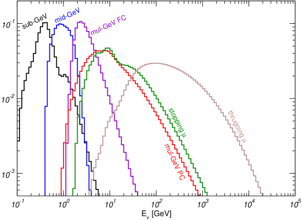
where gives the contribution of the neutrino flux of energy to the event rate after weighting with the neutrino interaction cross sections, muon propagation and detection efficiencies. In order to illustrate which part of the atmospheric neutrino spectrum is mostly determined by each event type we plot in Fig. 1 the function (normalized to one) for the Honda atmospheric fluxes [6], for each event type – Sub-GeV, Mid-GeV and Multi-GeV, partially contained, stopping and thrugoing muon events– averaged over zenith angle (assuming oscillations with eV2 and ). In particular from the figure we note that for energies larger than few TeV and smaller than GeV there is essentially no information on the atmospheric neutrino flux coming from the available event rates.
The experimental correlation matrix for the event rates is constructed in the following way:
| (5) |
where the statistical uncertainty is given by
| (6) |
and the correlated uncertainties are computed from the couplings factors, to the corresponding pull [29],
| (7) |
The couplings used in the analysis are a generalization of those given in Ref. [30] to include the separation between sub-GeV and mid-GeV and the partially contained samples, and will be described in more detail in a forthcoming publication.
In particular, we consider three different sets of correlated errors:
-
1.
Experimental systematic uncertainties (exp), like uncertainty in the detector calibration and efficiency.
-
2.
Theoretical cross-section uncertainties (cross), like cross-section normalization errors and cross section ratios errors.
-
3.
Theoretical zenith angle and flavor flux uncertainty (flx).
Note that in standard neutrino oscillation parameter global fits like [3], the flux uncertainties include on top of the above a flux normalization and a flux tilt errors, but in our case we do not have to include them because we are determining the energy dependence of the atmospheric flux (including its normalization) directly from the neutrino data. In other words, since our objective is to establish how well we can determine the normalization and energy dependence of the flux directly from the data, nothing is assumed about them: neither their values nor their theoretical uncertainties. We will go back to this point after Eq. (12).
Finally the total error is computed adding the statistical and correlated errors in quadrature
| (8) |
We summarize the characteristic values of the uncertainties in the different data samples in Table 1. From the table we see that the experimental statistical errors are more important in the high energy samples while the correlations are dominated by the cross section uncertainties.
| exp | exp+cross | exp+cross+flx | ||||||||
| Sub-GeV | 0.07 | 0.01 | 0.08 | 0.21 | 0.15 | 0.17 | 0.83 | 0.15 | 0.17 | 0.84 |
| Sub-GeV | 0.09 | 0.01 | 0.09 | 0.20 | 0.15 | 0.17 | 0.79 | 0.15 | 0.18 | 0.79 |
| Mid-GeV | 0.08 | 0.01 | 0.08 | 0.21 | 0.10 | 0.13 | 0.69 | 0.11 | 0.13 | 0.69 |
| Mid-GeV | 0.07 | 0.01 | 0.07 | 0.21 | 0.11 | 0.13 | 0.74 | 0.11 | 0.13 | 0.74 |
| Multi-GeV | 0.12 | 0.03 | 0.12 | 0.24 | 0.09 | 0.15 | 0.50 | 0.10 | 0.16 | 0.51 |
| Multi-GeV | 0.13 | 0.03 | 0.13 | 0.23 | 0.10 | 0.16 | 0.49 | 0.11 | 0.17 | 0.50 |
| PC | 0.11 | 0.06 | 0.13 | 0.40 | 0.12 | 0.16 | 0.62 | 0.12 | 0.16 | 0.68 |
| Stop | 0.16 | 0.07 | 0.17 | 0.30 | 0.10 | 0.19 | 0.41 | 0.10 | 0.19 | 0.41 |
| Thru | 0.08 | 0.02 | 0.08 | 0.23 | 0.09 | 0.12 | 0.66 | 0.10 | 0.13 | 0.67 |
| Total | 0.10 | 0.03 | 0.11 | 0.03 | 0.11 | 0.15 | 0.35 | 0.12 | 0.16 | 0.36 |
The purpose of the artificial data generation is to produce a Monte Carlo set of ‘pseudo–data’, i.e. replicas of the original set of data points:
| (9) |
such that the sets of points are distributed according to an –dimensional multi-gaussian distribution around the original points, with expectation values equal to the central experimental values, and error and covariance equal to the corresponding experimental quantities.
This is achieved by defining
| (10) |
where is the number of generated replicas of the experimental data, and where are univariate gaussian random numbers with the same correlation matrix as experimental data, that is they satisfy
| (11) |
Because [31] the distribution of the experimental data coincides (for a flat prior) with the probability distribution of the value of the event rate at the points where it has been measured, this Monte Carlo set gives a sampling of the probability measure at those points.
Note that all errors considered (including correlated systematics and theoretical uncertainties) must be treated as gaussian in this framework. However, this does not imply that the resulting flux probability density is gaussian, since the Monte Carlo method allows for a non-gaussian distribution of best-fit atmospheric neutrino flux distributions to be obtained as a result of the fitting procedure.
We can then generate arbitrarily many sets of pseudo–data, and choose the number of sets in such a way that the properties of the Monte Carlo sample reproduce those of the original data set to arbitrary accuracy. The relevant issue at this point is to determine the minimum number of replicas required to reproduce the properties of the original data set with enough accuracy.
In our particular case we have generated two different samples of replicas, each with one different set of correlated uncertainties, as described above, exp+cross, and exp+cross+flx. A fit including the exp uncertainties only is meaningless since the results of the Super-Kamiokande experiment are not consistent with the neutrino oscillation hypothesis (since the overall is too high) and with the results of K2K and MINOS (since the preferred is too low) if both flux and cross-section uncertainties are simultaneously neglected [35]. The features of the Monte Carlo generated replicas with these two types of uncertainties included in the generation are summarized in terms of several statistical estimators (see Appendix A for definitions) in Table 2.
These statistical estimators allow us to assess in a quantitative way if the Monte Carlo sample of replicas reproduces the features of the experimental data. For example, we can check that averages, variance and covariance of the pseudo-data reproduce central values and covariance matrix elements of the original data. From the table we see that for the two sets of uncertainties considered, 100 replicas are enough to reproduce the properties of the original data set with the required accuracy, namely a few percent, which is the accuracy of the experimental data while it is clear that 10 replicas fall short to reproduce the statistical properties of the experimental data.
| exp+cross | exp+cross+flx | ||
| 100 | 100 | 10 | |
| 1.5% | 1.5% | 4.7% | |
| 0.99 | 0.99 | 0.99 | |
| 10.5% | 9.6% | 10.1% | |
| 18.1 | 18.5 | 18.5 | |
| 17.5 | 18.9 | 13.8 | |
| 0.99 | 0.99 | 0.76 | |
| 0.35 | 0.36 | 0.36 | |
| 0.34 | 0.34 | 0.26 | |
| 0.94 | 0.94 | 0.36 | |
| 137.6 | 145.7 | 145.7 | |
| 122.7 | 129.2 | 53.2 | |
| 0.98 | 0.98 | 0.42 | |
2.2 Neural Network Training
The second step consists of training neural networks. In our case each neural network parametrizes a differential flux, which in principle should depend on the neutrino energy , the zenith angle and the neutrino type ( labels the the neutrino flavor: electron neutrinos and antineutrinos, and muon neutrinos and antineutrinos), and is based on all the data in one single replica of the original data set. However, the precision of the available experimental data is not enough to allow for a separate determination of the energy, zenith angle and type dependence of the atmospheric flux. Consequently in this work we will assume the zenith and type dependence of the flux to be known with some precision and extract from the data only its energy dependence. Thus the neural flux parametrization will be:
| (12) |
where is the neural network output when the input is the neutrino energy
| (13) |
and it depends on the neutrino energy333In fact the input variable is rather , since it can be shown [33] that an appropriate preprocessing of the input parameters speeds up the training process. as well as on the parameters of the neural network (see Appendix C for details). In Eq. (12) is a reference differential flux, which we take to be the most recent computations of either the Honda [6] or the Bartol [7] collaborations, extended to cover also the high-energy region by consistent matching with the Volkova fluxes [34]. Notice that in what respects the normalization and energy dependence of the fluxes, the choice of reference flux is irrelevant. Any variation on the normalization or on the energy dependence of the reference flux can be compensated by the corresponding variation of so that the output flux will be the same. The dependence of the results of the analysis on the reference flux comes because of the differences among the different flux calculations in angular and flavour dependence.
Nothing further is assumed about the function whose value is only known after the full procedure of training of the neural net is finished. There are, however, some requirements about the choice of the architecture of the neural network. As discussed in Refs. [20, 21] such choice cannot be derived from general rules and it must be tailored to each specific problem. The main requirements for an optimal architecture are first of all that the net is large enough so that the results are stable with respect small variations of the number of neurons (in this case the neural net is called redundant) and, second, that this net is not so large than the training times become prohibitive. For our problem the neural network must have a single input neuron (whose value is )) and a final output neuron (whose value is the ) and a number of hidden layers with several neurons each (see appendix C for further details). We have checked that an architecture with two hidden layers with 5 neurons each, i.e. a 1-5-5-1 network, satisfies the above requirements in the present case.
The process which determines the function which better describes each of the sets of artificial data, , is what we call training of the neural network. It involves two substeps. First for a given the expected atmospheric event rates have to be computed in a fast an efficient way. Second the neural network parameters have to be determined by minimizing some error function. We describe them next.
2.2.1 From Atmospheric Fluxes to Event Rates
The expected event rate for contained and upgoing muon events for a given set of neural network parameters , or what is the same for a given value of the neural network flux, can be obtained by substituting Eq. (12) into Eqs. (2) and (3) respectively. However, from a practical point of view the above expressions are very time-consuming to evaluate, and this is a very serious problem in our case since in the neural network approach one requires a very large number of evaluations in the training process.
The procedure can be speed up if one realizes that for a given flux the expected event rates can always be written as
| (14) |
where labels both the flavor and the chirality of the initial neutrino state. Comparing Eq. (14) with Eqs. (2) and (3) we get:
| (15) |
for contained events, and
| (16) |
for upgoing-muon events. Consequently, if one discretizes the differential fluxes in energy intervals and zenith angle intervals one can write
| (17) | |||
| (18) |
and therefore it is possible to write the theoretical predictions as a sum of the elements of the discretized flux table,
| (19) |
where the coefficients , which are the most time-consuming ingredient, need only to be precomputed once before the training, since they do not depend on the parametrization of the atmospheric neutrino flux.
In our calculations we have used energy intervals, equally spaced between and (with in GeV) and bins in zenith angle, equally spaced between and so
| (20) |
where the integrations in Eq. (20) are performed via Monte Carlo numerical integration.
2.2.2 Minimization Procedure
From each replica of artificial data an atmospheric neutrino flux parametrized with a neural network is obtained. The data points in each replica are used to determine the parameters of the associated neural net. The fit of the fluxes to each replica of the data, or what is the same, the determination of the parameters that define the neural network, its weights, is performed by maximum likelihood. This procedure, the so-called neural network training, proceeds by minimizing an error function , which coincides with the of the experimental points when compared to their theoretical determination obtained using the given set of fluxes:
| (21) |
The case corresponds to the experimental values, . The has to be minimized with respect to , the parameters of the neural network.
We perform two different type of fits which we denote by exp+cross and exp+cross+flx. To be consistent we include in each one the same correlated uncertainties that have been included in the replica generation. For example, if we want to include only the effects of the exp+cross uncertainties, in Eqs. (5) and (8) the sum includes only experimental systematic and theoretical cross section uncertainties, while in Eq. (21) one imposes for flx uncertainties.
Unlike in conventional fits with errors, however, the covariance matrices of the best–fit parameters are irrelevant and need not be computed. The uncertainty on the final result is found from the variance of the Monte Carlo sample. This eliminates the problem of choosing the value of which corresponds to a one-sigma contour in the space of parameters.
Rather, one only has to make sure that each neural net provides a consistent fit to its corresponding replica. If the underlying data are incompatible or have underestimated errors, the best fit might be worse than one would expect with properly estimated gaussian errors — for instance in the presence of underestimated errors it will have typically a value of per degree of freedom larger than one. However, neural nets are ideally suited for providing a fit in this situation, based on the reasonable assumption of smoothness: for example, incompatible data or data with underestimated errors will naturally be fitted less accurately by the neural net. Also, this allows for non-gaussian behavior of experimental uncertainties.
The minimization of Eq. (21) is performed with the use of genetic algorithms (summarized in Appendix D, see Ref. [21] and references therein for a more complete description). Because of the nonlinear dependence of the neural net on its parameters, and the nonlocal dependence of the measured quantities on the neural net (event rates are given by multi-dimensional convolutions of the initial flux distributions), a genetic algorithm turns out to be the most efficient minimization method. The use of a genetic algorithm is particularly convenient when seeking a minimum in a very wide space with potentially many local minima, because the method handles a population of solutions rather than traversing a path in the space of solutions.
The minimization is ended after a number of iterations of the minimization algorithm large enough so that of Eq. (21) stops decreasing, that is, when the fit has converged.444Note that the standard criterion to stop neural network training, the overlearning criterion, cannot be used in our case due to the scarce amount of data. Thus an important issue in the procedure is to determine the right number of iterations which should be used. In order to determine them, we define the total ,
| (22) |
with the event rates computed as an average over the sample of trained neural nets,
| (23) |
and we study its value as a function of the number of iterations used in the minimization.
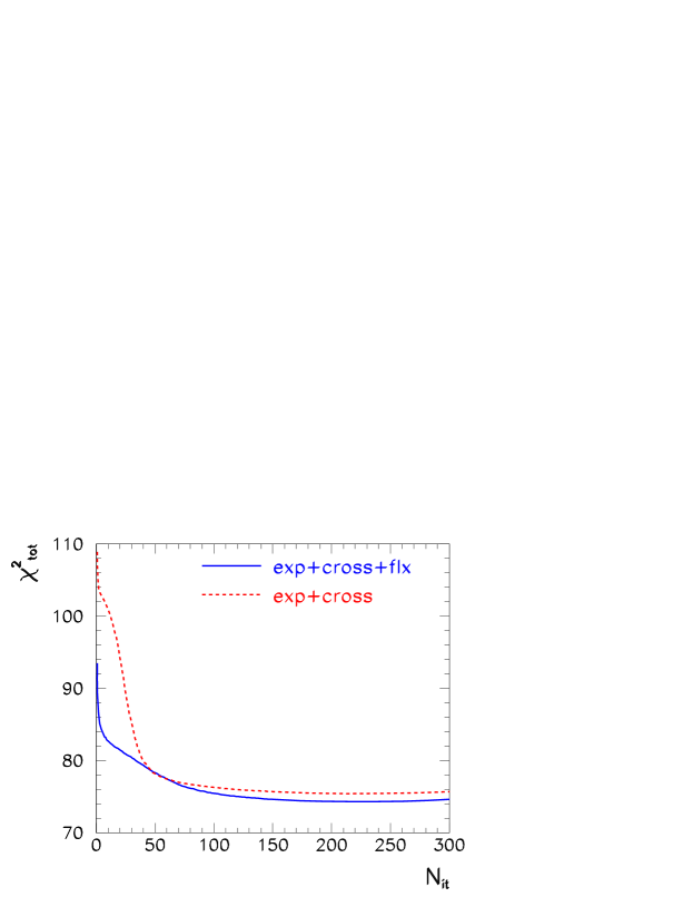
We show in Fig. 2 the dependence of on the number of minimization iterations, in the two cases considered. From the figure we see that the number of iterations needed to achieve convergence can be safely taken to be both for the in the exp+cross and exp+cross+flx fits.
Thus at the end of the procedure, we end up with fluxes, with each flux given by a neural net. The set of fluxes provide our best representation of the corresponding probability density in the space of atmospheric neutrino fluxes: for example, the mean value of the flux at a given value of is found by averaging over the replicas, and the uncertainty on this value is the variance of the values given by the replicas. Generally, we expect the uncertainty on our final result to be somewhat smaller than the uncertainty on the input data, because the information contained in several data points is combined.
There are two type of tests that can be performed on the properties of this probability measure. First, the self-consistency of the Monte Carlo sample can be tested in order to ascertain that it leads to consistent estimates of the uncertainty on the final set of fluxes, for example by verifying that the value of the flux extracted from different replicas indeed behaves as a random variable with the stated variance. This set of tests allows us to make sure that the Monte Carlo sample of neural nets provides a faithful and consistent representation of the information contained in the data on the probability measure in the space of fluxes, and in particular that the value of fluxes and their (correlated) uncertainties are correctly estimated.
Furthermore the properties of this measure can be tested against the input data by using it to compute means, variance and covariances which can be compared to the input experimental ones which have been used in the flux determination.
3 Results for the Reference Fit
In this section we discuss our results for the reference fit of the atmospheric neutrino fluxes. For this fit we use the Honda [6] flux as reference, the exp+cross+flx set of uncertainties. and we assume oscillations with oscillation parameters and . We will discuss in next section the dependence of the results on these choices.
As described in the previous section, we start by generating a set of replicas of the experimental data points according to Eq. (10) where in we include both the statistical as well as the correlated errors from experimental systematic uncertainties, theoretical cross section uncertainties and the theoretical flux uncertainties in the angular distributions and neutrino type ratios. As shown in Table 2, this Monte Carlo sample of replicas reproduces with enough precision the statistical features of the original experimental data.
After that we proceed to the training of the neural networks as described in Sec. 2.2. Once the training of the sample of neural networks has been completed, we obtain the set of fluxes which provide us with the probability density in the space of atmospheric neutrino fluxes. In particular we compute the average atmospheric neutrino flux as
| (24) |
and the standard deviation as
| (25) |
for any given value of the energy , the zenith angle and the neutrino type .
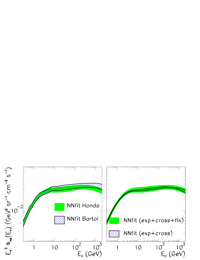
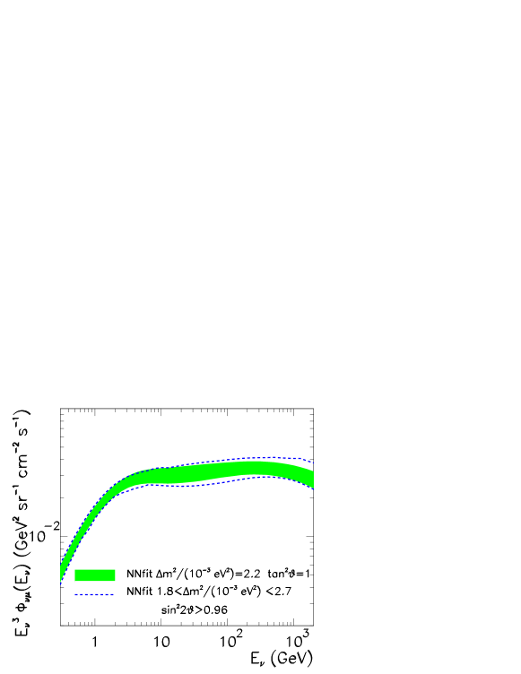
In Fig. 3 we show the results for the flux (in particular we show the angular averaged muon neutrino flux) as compared with the computations of the Honda [6] and Bartol [7] groups. The results of the neural network fit are shown as the band as a function of the neutrino energy. We see from the figure that the flux obtained from this fits is in reasonable agreement with the results from the the calculations of Honda and Bartol groups. We also see that at lower energies the present uncertainty in the extracted fluxes is larger than the range of variations between calculations while at higher energies the opposite holds. The fit also seems to prefer a slightly higher flux at higher energies.
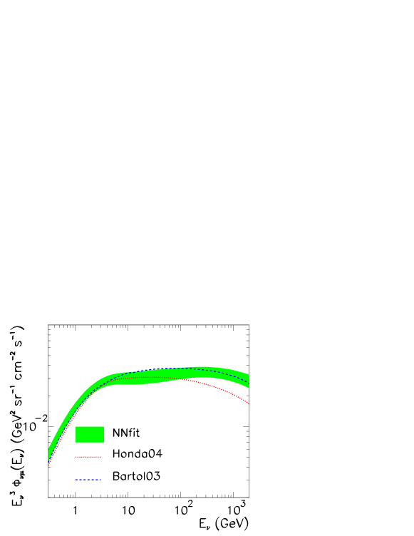
The statistical estimators for this reference training are given in the first column in Table 3, where the different estimators can be found in Appendix A. Note that errors are somewhat reduced, as expected if the neural network has found the underlying physical law, correlations increase and covariances are appropriately reproduced, a sign that the sample of trained neural networks correctly reproduces the probability measure that underlies experimental data. We will return to the discussion on error reduction in next section.
| Fit | Reference | Bartol Flux | exp+cross |
|---|---|---|---|
| 74.6 | 73.3 | 75.7 | |
| 8.9% | 9.1% | 9.0% | |
| 0.99 | 0.98 | 0.99 | |
| 18.5 | 18.5 | 18.1 | |
| 14.7 | 14.7 | 3.2 | |
| 0.97 | 0.98 | 0.81 | |
| 0.36 | 0.36 | 0.35 | |
| 0.65 | 0.66 | 0.78 | |
| 0.69 | 0.71 | 0.74 | |
| 145.7 | 145.7 | 137.6 | |
| 136.0 | 131.8 | 8,5 | |
| 0.95 | 0.97 | 0.78 |
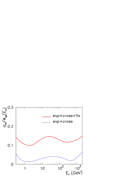
In Fig. 4, we plot the relative error as function of the energy which, as seen in the figure, grows at the lowest and highest energies. The fact that the relative error grows in the region where less data is available reflects the fact that the behavior of neural networks in those regions is not determined by its behavior in the regions where more data is available, as it would happen in fits with usual functional forms.
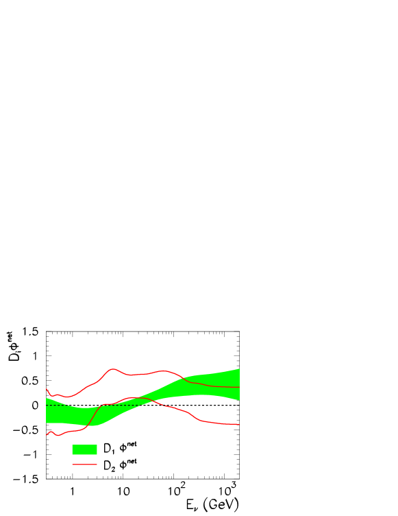
The first and second derivatives of the flux ratio with the associated uncertainties,
| (26) | ||||
| (27) |
are shown in Fig. 5. From the figure we see that, within the present errors, the first derivative is not a constant, or in other words one cannot parametrize the energy dependence of the flux uncertainty as a simple tilt correction,
| (28) |
However, we also see that the second derivative is compatible with zero within errors in almost all the energy range, which implies that the uncertainty is not a much more strongly varying function of the energy.
Finally from Eq. (19) we compute the predicted event rates for the fluxes and define their average as in Eq. (23) and their standard deviation as
| (29) |
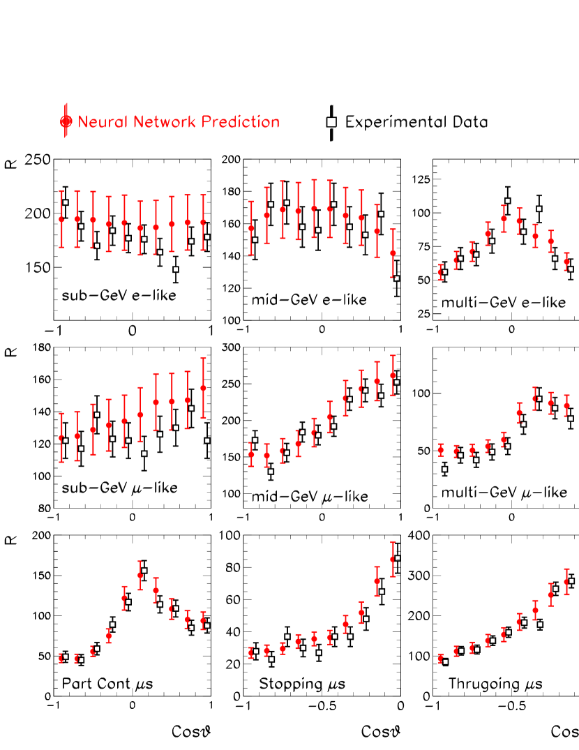
In Fig. 6 we show a comparison of the experimental data with the corresponding predictions of the neural network parametrization of the atmospheric neutrino flux. From the figure we see that the predicted rates are in good agreement with the data, but, as expected, have a smoother zenith angular dependence.
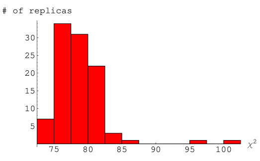
Another interesting figure of merit to verify the correct statistical behavior of the neural network training is the distribution of , defined as the of the set of neural fluxes compared to experimental data, that is
| (30) |
This distribution is shown in Fig. 7. Note that for all the fluxes . Furthermore, if we define , where is the maximum value of the set of 68% fluxes with lower ,we get that in the present analysis the 1- range of fluxes obtained from the sample of trained neural networks corresponds to , which satisfies as expected for a consistent distribution of fits.
4 Stability of the Results
In this section we discuss the stability of our results with respect to different inputs used for the reference fit, such as some of the choices in the training procedure, the assumptions made on the zenith angle and flavor dependence of the atmospheric fluxes, and the uncertainty on the neutrino oscillation parameters.
4.1 Impact of Training Choices
In order to verify the stability of the results with respect to the minimization algorithm used in the neural network training procedure first of all we have repeated the fit using genetic algorithms but with a larger number of iterations (=300). The results are shown in Fig. 8. We see that this increase in the number of iterations does not lead to any substantial variation of the allowed range of fluxes. This implies that the minimization had indeed converged well before as it was illustrated in Fig. 2.

Second, we have repeated the fit by using dynamical stopping of the training as alternative minimization strategy. In dynamical stopping, instead of training each neural net a fixed number of iterations, the training of each net is stopped independently when a certain condition on the error function is satisfied. In particular, in this training strategy one fixes a parameter and then stops the fit to each replica separately when the condition is satisfied, with as stated in Eq. (21). It can be shown [20] that the typical values for , are of the order of . Therefore each different value of will result in a different value of the total , Eq. (22). Clearly one expects that the higher the value of the larger the flux error ranges. Thus to make the comparison meaningful we must chose a value of which leads to a of comparable value of the one obtained in the reference fit. We have verified that for , which is close enough to the reference fit value . The results for this alternative fit are shown in Fig. 8. Again we see that the results obtained with both minimization strategies are very compatible. The main effect of using dynamical stopping is a slight increase of the allowed range of fluxes in the intermediate energy region.
Finally, as a consistency check, we have verified that the obtained energy dependence in a given energy range is mostly determined by the data sample which is most sensitive to that energy range. We have done so by repeating the reference fit but removing the thrugoing muon sample in the analysis. The results are shown in Fig. 8 where we see that, while the fit is unaltered at lower energies, the results get considerably different for neutrinos with energies GeV which are the ones responsible for thrugoing neutrino events as illustrated in Fig. 1. Basically once the thrugoing muon sample is removed from the fit, we have no experimental information for GeV. Consequently the results of the fit at those higher energies are just an unphysical extrapolation of the fit at lower energies as clearly illustrated in the figure where we see that there is no lower bound to the allowed flux at those higher energies.
This reflects the fact that the behavior of neural networks in the extrapolation region is not determined by its behavior where more data is available, as it would happen in fits with usual functional forms. In principle, if the neural network had found some underlying physical law which described the experimental data and which would be valid both in the region where data is available and in the extrapolation region, the value of the extrapolated fluxes could be less unconstrained. However, this is not expected in this case since it is precisely at energies of the order of GeV that the start interacting before they are able to decay which implies that the underlying physical law is different below and above those energies, and the extrapolation is therefore very much unconstrained.
4.2 Impact of Choice for Zenith Angle and Flavor Flux Dependence
As previously discussed, since the available experimental data from Super-Kamiokande are not precise enough to allow for a simultaneous independent determination of all the elements in the atmospheric neutrino fluxes, we have restricted our analysis to the determination of their energy dependence, and taken the zenith angle and flavor dependence from a previous computation [6].
In order to assess the effects of this choice we first repeat the reference fit but using as reference flux the Bartol flux [7]. In the left panel of Fig. 9 we compare the results of these two fits. We see that the results are identical for GeV as expected since both Honda and Bartol calculations give very similar angular and flavour ratios at those energies. And for any energy the difference between the results of both fits are much smaller than the differences between the reference fluxes themselves, see Fig. 3. This is what is expected since the flx uncertainties included in both fits represent the spread on the theoretical flux calculations of the angular dependence and flavour ratios.
In the second column in Table 3 we give the statistical estimators corresponding to the fit taking Bartol as a reference flux. As expected the differences with results using Honda as reference flux (first column in Table 3) are very small.
The importance of the choice of angular and flavour dependence can also be addressed by studying the effect of removing from the analysis the flx errors since those errors account for the spread of the predicted angular and flavour dependence among the different atmospheric flux calculations. In other words removing those errors we force the neural net flux to follow the angular and flavour dependence of the reference flux without allowing for any fluctuation about them. The results of this fit and its comparison with the reference fit are shown in the right panel of Fig. 9. The corresponding statistical estimators are given in the third column of Table 3 while in Fig. 10 we show the neural network predictions for the event rates in this case.
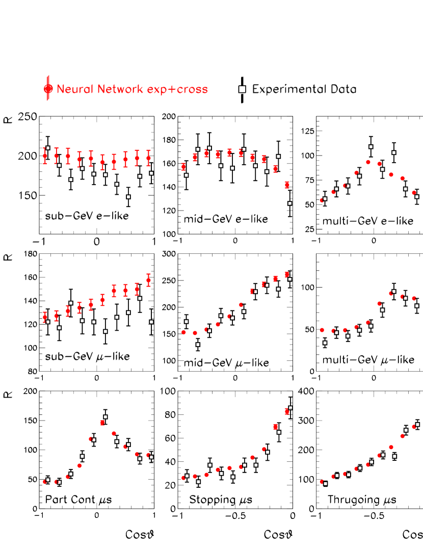
As expected, (see Table 3) is larger once the flx errors are not included in the fit, although given the small size of the flx errors this increase is very moderate (only 1.1 units for 90 data points). Equivalently from Table 3 we see the small impact that the exclusion of the flx errors makes in the evaluation of the statistical estimators of the experimental data , , and which is again a reflection of the small values of the flx compared to the experimental statistical and systematic uncertainties.
There is, however, a much more important effect in the size of the allowed range of fluxes and predicted rates in as seen in Figs. 9 and 10. As shown in Fig. 4 the relative error of the flux is reduced by a factor – in the full energy range. At first this considerable reduction of the relative flux error when removing only the relatively small flx uncertainties may seem counterintuitive. However this result is expected if the results of the fit are consistent. This is because the zenith and flavor dependence is not fitted from data. As a consequence, if no uncertainties are included associated with those, there are or binned rates of similar statistical weight (20 from the e-like and mu-like distributions for sub- mid- and multi-GeV events and 10 for partially contained, stopping and thrugoing muons) contributing to the determination of the flux in the same energy range with no allowed fluctuations among them. Thus the associated uncertainty in the determination of the energy dependence is indeed reduced by a factor –5. This is also reflected in Table 3, where we see that there is a reduction on the statistical estimators which measure the average spread of the predicted rates obtained when using the neural net fluxes, and .555Since is proportional to the square of the , the reduction in this case is a factor .
The inclusion of the flx uncertainties and their corresponding pulls allows for the angular and flavour ratio of the fitted fluxes to spread around their reference flux values. This results into an effective decoupling of the contribution of the data points to the fit at a given with the corresponding increase in the flux relative error. Furthermore once the flx uncertainties are included the range of the angular binned rate predictions are of the same order of the statistical error of the experimental points (see Fig. 1).
Finally let’s also point out that, in general, adding or removing some source of uncertainty does not only change the size of the associated errors in the parametrization but also the position of the minimum, that is, the features of the best-fit flux, although this effect is small in the present case.
4.3 Impact of Oscillation Parameters
So far the results presented for the different fits have been done assuming oscillations with oscillation parameters fixed to
| (31) |
In order to address the impact on the results of the assumed value of the oscillation parameters we repeat the fit with these parameters varying within their 1-sigma ranges as allowed by global fits to neutrino oscillations data. In particular we consider the range
| (32) |
The results are shown in Fig. 11 where we show the envelope of the results obtained varying each time one of the neutrino oscillation parameters. As we can see in Fig. 11, the contribution to the total error from the uncertainty in the neutrino oscillation parameters is rather small. Therefore we can be confident than the impact in our results of the uncertainties in the oscillation parameters is very small, and moreover this uncertainty can be systematically reduced as our knowledge of neutrino oscillation parameters increases.
5 Summary and Outlook
In this work we have presented the first results on the determination of the energy dependence of the atmospheric neutrino fluxes from the data on atmospheric neutrino event rates measured by the Super-Kamiokande experiment. In order to bypass the problem of the unknown functional form for the neutrino fluxes we have made use of artificial neural networks as unbiased interpolants. On top of this, a faithful estimation of the uncertainties of the neutrino flux parametrization has been obtained by the use of Monte Carlo methods.
In our analysis we have relied on the zenith and flavour dependence of the flux as predicted by some of the atmospheric flux calculations in Refs. [6, 7, 8]. Also, the fluxes are determined under the assumption that oscillation parameters will eventually be independently determined by non atmospheric neutrino experiments with a value close to the present best fit. We have estimated the uncertainties associate with these choices by performing alternative fits to the data where some of these assumptions were changed and/or relaxed.
Our main result is presented in Fig. 3. We have found that until about TeV we have a good understanding of the normalization of the fluxes and the present accuracy from Super-Kamiokande neutrino data is comparable with the theoretical uncertainties from the numerical calculations. The results of our alternative fits shows that if one assumes that the present uncertainties of the angular dependence have been properly estimated, it turns out that the assumed angular dependence has very little effect on the determination of the energy dependence of the fluxes. Thus the determined atmospheric neutrino fluxes could be used as an alternative of the existing flux calculations, and are available upon request to the authors.
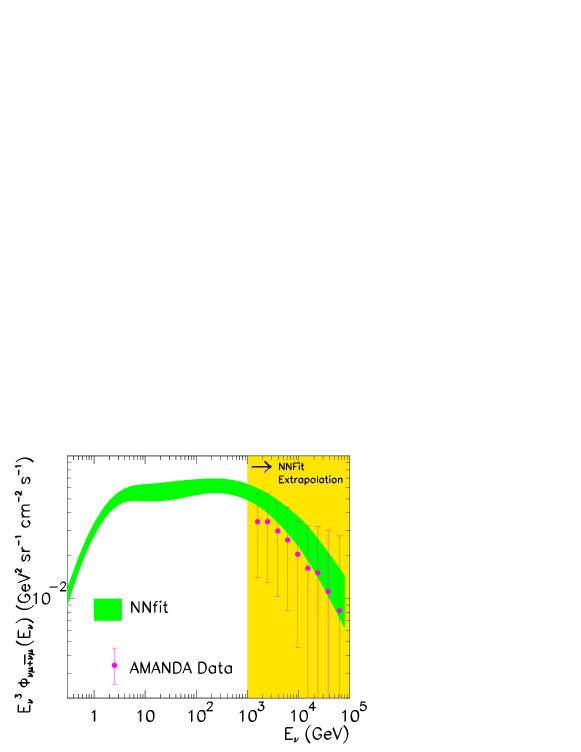
The results of this work can be extended in several directions. It would be interesting to include in the analysis the atmospheric neutrino data from detectors that probe the high energy region, like AMANDA [36, 37] or ICECUBE [38]. To illustrate the reach of the presently available statistics at those energies we show in Fig. 12 the results for the reference fit for the angular averaged muon neutrino plus antineutrino flux extrapolated to the high energy region compared to the data from AMANDA [36, 37]. Notice that, as mentioned above, the behavior of neural networks in the extrapolation region is not determined by its behavior where data is available, as it would happen in fits with usual functional forms. As a consequence the values of the extracted fluxes in the extrapolation region can be extremely unphysical as described in Sec. 4.1. To improve the extrapolation, one could use high-energy functional forms for the atmospheric neutrino flux, for example those presented in [39], which have been used in [40] to fit analytical expressions for the fluxes to the Monte Carlo simulations. The implementation of this strategy is postponed to future work, when also the AMANDA and ICECUBE atmospheric neutrino data will be incorporated in the fit.
Furthermore one could assess the effects of determining from experimental data the full energy, zenith and flavor dependence of the atmospheric neutrino fluxes together with the oscillation parameters, in particular in the context of the expected data from future megaton neutrino detectors [15, 16].
Acknowledgments.
We thank F. Halzen for comments and careful reading of the manuscript. J. R. would like to acknowledge the members of the NNPDF Collaboration: Luigi del Debbio, Stefano Forte, Jose Ignacio Latorre and Andrea Piccione, since a sizable part of this work is related to an upcoming common publication [24]. M.C. G-G would like to thank the CERN theory division for their hospitality during the weeks previous to the finalization of this work. This work is supported by National Science Foundation grant PHY-0354776 and by Spanish Grants FPA-2004-00996 and AP2002-2415.Appendix A Statistical Estimators
In this Appendix we summarize the estimators used to validate the generation of the Monte Carlo sample of replicas of the experimental data. The corresponding estimators that validate the neural network training can be straightforwardly obtained by replacing the superscript with .
-
•
Average over the number of replicas for each experimental point
(33) -
•
Associated variance
(34) -
•
Associated covariance
(35) (36) The three above quantities provide the estimators of the experimental central values, errors and correlations which one extracts from the sample of experimental data.
-
•
Mean variance and percentage error on central values over the data points.
(37) (38) We define analogously , , and , and , for errors, correlations and covariances respectively.
These estimators indicate how close the averages over generated data are to the experimental values. Note that in averages over correlations and covariances one has to use the fact that correlation and covariances matrices are positive definite, and thus one has to be careful to avoid double counting. For example, the percentage error on the correlation will be defined as
(39) and similarly for averages over elements of the covariance matrix.
-
•
Scatter correlation:
(40) where the scatter variances are defined as
(41) (42) We define analogously , and . Note that the scatter correlation and scatter variance are not related to the variance and correlation Eqs. (34)-(36). The scatter correlation indicates the size of the spread of data around a straight line. Specifically implies that is proportional to .
-
•
Average variance:
(43) We define analogously and , as well as the corresponding experimental quantities. These quantities are interesting because even if are close to 1 there could still be a systematic bias in the estimators Eqs. (34)-(36). This is so since even if all scatter correlations are very close to 1, it could be that some of the Eqs. (34)-(36) where sizably smaller than its experimental counterparts, even if being proportional to them.
The typical scaling of the various quantities with the number of generated replicas follows the standard behavior of gaussian Monte Carlo samples. For instance, variances on central values scale as , while variances on errors scale as . Also, because
| (44) |
the estimated correlation fluctuates more for small values of , and thus the average correlation tends to be larger than the corresponding experimental value.
Appendix B The Monte Carlo Approach to Error Estimation
In this Appendix we show with a simple example how the Monte Carlo approach to error estimation is equivalent to the standard approach, based on the condition for the determination of confidence levels, with the assumption of gaussian errors, up to linearized approximations. For a more detailed analysis of this statistical technique the reader is referred to [31].
Let us consider two pairs of independent measurements of the same quantity, and with gaussian uncertainties. The distribution of true values of the variable is a gaussian distribution centered at
| (45) |
and with variance determined by the tolerance criterion,
| (46) |
To obtain the above results, note that if errors are gaussianly distributed, the maximum likelihood condition implies that the mean minimizes the function
| (47) |
and the variance is determined by the condition
| (48) |
which for leads to Eq. (46). Note that these properties only hold for gaussian measurements.
An alternative way to compute the mean and the variance of the combined measurements and is the Monte Carlo method: generate replicas of the pair of values gaussianly distributed with the appropriate error,
| (49) | |||
| (50) |
where are univariate gaussian random numbers. One can then show that for each pair, the weighted average
| (51) |
is gaussianly distributed with central value and width equal to the one determined in the previous case. That is, it can be show that for a large enough value of ,
| (52) |
and for the variance
| (53) |
which is the same result, Eq. (46), as obtained from the criterion. This shows that the two procedures are equivalent in this simple case.
The generalization to gaussian correlated measurements is straightforward. Let us consider for instance that the two measurements and are not independent, but that they have correlation . To take correlations into account, one uses the same Eqs. (49) and (50) to generate the sample of replicas of the measurements, but this time the random numbers and are univariate gaussian correlated random numbers, that is, they satisfy
| (54) |
With this modification, the sample of Monte Carlo replicas of and also reproduces the experimental correlations. This can be seen with the standard definition of the correlation,
| (55) |
Therefore, the Monte Carlo approach also correctly takes into account the effects of correlations between measurements.
In realistic cases, the two procedures are equivalent only up to linearizations of the underlying law which describes the experimental data. We take the Monte Carlo procedure to be more faithful in that it does not involve linearizing the underlying law in terms of the parameters. Note that as emphasized before, the error estimation technique that is described in this thesis does not depend on whether one uses neural networks or polynomials as interpolants.
Appendix C Neural Network Details
Artificial neural networks [32, 33] provide unbiased robust universal approximates to incomplete or noisy data. An artificial neural network consists of a set of interconnected units (neurons). The activation state of a neuron is determined as a function of the activation states of the neurons connected to it. Each pair of neurons is connected by a synapses, characterized by a weight . In this work we will consider only multilayer feed-forward neural networks. These neural networks are organized in ordered layers whose neurons only receive input from a previous layer. In this case the activation state of a neuron in the (l+1)-th layer is given by
| (56) | |||
| (57) |
where is the activation threshold of the given neuron, is the number of neurons in the l-th layer, is the number of layers that the neural network has, and is the activation function of the neuron, which we will take to be a sigma function,
| (58) |
except in the last layer, where we use a linear activation function . This enhances the sensitivity of the neural network, avoiding the saturation of the neurons in the last layer. The fact that the activation function is non-linear allows the neural network to reproduce nontrivial functions.
Therefore multilayer feed-forward neural networks can be viewed as functions parametrized by weights, thresholds and activation functions,
| (59) |
It can be proved that any continuous function, no matter how complex, can be represented by a multilayer feed-forward neural network. In particular, it can be shown [32, 33] that two hidden layers suffice for representing an arbitrary function.
In our particular case the architecture of the neural network used is 1-5-5-1, which means that it has a single input neuron (whose value is the neutrino energy), two hidden layers with 5 neurons each and a final output neuron (whose value is the atmospheric neutrino flux).
Appendix D Genetic Algorithms
Genetic algorithms are the generic name of function optimization algorithms that do not suffer of the drawbacks that deterministic minimization strategies have when applied to problems with a large parameter space. This method is specially suitable for finding the global minima of highly nonlinear problems.
All the power of genetic algorithms lies in the repeated application of two basic operations: mutation and selection. The first step is to encode the information of the parameter space of the function we want to minimize into an ordered chain, called chromosome. If is the size of the parameter space, then a point in this parameter space will be represented by a chromosome,
| (60) |
In our case each bit of a chromosome corresponds to either a weight or a threshold of a neural network. Once we have the parameters of the neural network written as a chromosome, we replicate that chain until we have a number of chromosomes. Each chromosome has an associated fitness , which is a measure of how close it is to the best possible chromosome (the solution of the minimization problem under consideration). In our case, the fitness of a chromosome is given by the inverse of the function to minimize, given in Eq. (21).
Then we apply the two basic operations:
-
•
Mutation: Select randomly a bit (an element of the chromosome) and mutate it. The size of the mutation is called mutation rate , and if the k-th bit has been selected, the mutation is implemented as
(61) where is a uniform random number between 0 and 1. The optimal size of the mutation rate must be determined for each particular problem, or it can be adjusted dynamically as a function of the number of iterations.
-
•
Selection: Once mutations and crossover have been performed into the population of individuals characterized by chromosomes, the selection operation ensures that individuals with best fitness propagate into the next generation of genetic algorithms. Several selection operators can be used. The simplest method is to select simply the chromosomes, out of the total population of individuals, with best fitness.
The procedure is repeated iteratively until a suitable convergence criterion is satisfied. Each iteration of the procedure is called a generation. A general feature of genetic algorithms is that the fitness approaches the optimal value within a relatively small number of generations, as seen in Fig. 2 for the present problem.
References
- [1] M. C. Gonzalez-Garcia and Y. Nir, Developments in neutrino physics, Rev. Mod. Phys. 75 (2003) 345–402, [hep-ph/0202058].
- [2] Frejus Collaboration, Determination of the atmospheric neutrino spectra with the Frejus detector, K. Daum et al., Z. Phys. C66, 417 (1995); Nusex Collaboration, Experimental study of atmospheric neutrino flux in the NUSEX experiment , M. Aglietta et al., Europhys. Lett. 8, 611 (1989); IMB Collaboration, R. Becker-Szend et al., The Electron-neutrino and muon-neutrino content of the atmospheric flux, Phys. Rev. D46, 3720 (1992); Kamiokande Collaboration, Y. Fukuda et al., Atmospheric muon-neutrino / electron-neutrino ratio in the multi-Gev energy range Phys. Lett. B335, 237 (1994).
- [3] Super-Kamiokande Collaboration, Y. Ashie et al., A measurement of atmospheric neutrino oscillation parameters by Super-Kamiokande I, Phys. Rev. D71 (2005) 112005, [hep-ex/0501064].
- [4] MACRO Collaboration, G. Giacomelli and A. Margiotta, New Macro results on atmospheric neutrino oscillations, Phys. Atom. Nucl. 67 (2004) 1139–1146, [hep-ex/0407023].
- [5] Soudan 2 Collaboration, M. C. Sanchez et al., Observation of atmospheric neutrino oscillations in Soudan 2, Phys. Rev. D68 (2003) 113004, [hep-ex/0307069].
- [6] M. Honda, T. Kajita, K. Kasahara, and S. Midorikawa, A new calculation of the atmospheric neutrino flux in a 3- dimensional scheme, Phys. Rev. D70 (2004) 043008, [astro-ph/0404457].
- [7] G. D. Barr, T. K. Gaisser, P. Lipari, S. Robbins, and T. Stanev, A three-dimensional calculation of atmospheric neutrinos, Phys. Rev. D70 (2004) 023006, [astro-ph/0403630].
- [8] G. Battistoni, A. Ferrari, T. Montaruli and P. R. Sala, The FLUKA atmospheric neutrino flux calculation, Astropart. Phys. 19 (2003) 269, [Erratum-ibid. 19 (2003) 291] [hep-ph/0207035]; Y. Liu, L. Derome and M. Buenerd, Atmospheric muon and neutrino flux from 3-dimensional simulation, Phys. Rev. D 67 (2003) 073022, [astro-ph/0211632]; J. Wentz, I. M. Brancus, A. Bercuci, D. Heck, J. Oehlschlager, H. Rebel and B. Vulpescu, Simulation of atmospheric muon and neutrino fluxes with CORSIKA, Phys. Rev. D67, (2003) 073020, [hep-ph/0301199];
- [9] T. K. Gaisser and M. Honda, Flux of atmospheric neutrinos, Ann. Rev. Nucl. Part. Sci. 52 (2002) 153–199, [hep-ph/0203272].
- [10] K2K Collaboration, E. Aliu et al., Evidence for muon neutrino oscillation in an accelerator-based experiment, Phys. Rev. Lett. 94, 081802 (2005). [hep-ex/0411038]
- [11] MINOS Collaboration, N. Tagg, First MINOS results from the NuMI beam, [hep-ex/0605058]
- [12] T2K Collaboration, Y. Yamada, T2K Phase-I And II, Nucl. Phys. Proc. Suppl. 155 (2006) 207.
- [13] D. A. Harris, Future experiments with neutrino superbeams, beta beams, and neutrino factories, Int. J. Mod. Phys. A19, 1201 (2004).
- [14] F. Halzen, Lectures on high-energy neutrino astronomy, astro-ph/0506248.
- [15] K. Nakamura, Hyper-Kamiokande: A next generation water cherenkov detector, Int. J. Mod. Phys. A18 (2003) 4053–4063.
- [16] UNO Proto-collaboration, UNO Whitepaper: Physics Potential and Feasibility of UNO, SBHEP-01- C. K. Jung, “Feasibility Of A Next Generation Underground Water Cherenkov Detector: Uno, AIP Conf. Proc. 533, 29 (2000) [hep-ex/0005046]
- [17] INO Collaboration, D. Indumathi, India-based neutrino observatory (ino), Pramana 63 (2004) 1283–1293.
- [18] R. K. Ellis, W. J. Stirling, and B. R. Webber, Qcd and collider physics, Camb. Monogr. Part. Phys. Nucl. Phys. Cosmol. 8 (1996) 1–435.
- [19] A. M. Cooper-Sarkar, R. C. E. Devenish, and A. De Roeck, Structure functions of the nucleon and their interpretation, Int. J. Mod. Phys. A13 (1998) 3385–3586, [hep-ph/9712301].
- [20] S. Forte, L. Garrido, J. I. Latorre, and A. Piccione, Neural network parametrization of deep-inelastic structure functions, JHEP 05 (2002) 062, [hep-ph/0204232].
- [21] J. Rojo, The neural network approach to parton distributions, PhD thesis, Universitat de Barcelona, 2006.
- [22] NNPDF Collaboration, L. Del Debbio, S. Forte, J. I. Latorre, A. Piccione, and J. Rojo, Unbiased determination of the proton structure function with faithful uncertainty estimation, JHEP 03 (2005) 080, [hep-ph/0501067].
- [23] A. Piccione, J. Rojo, L. Del Debbio, S. Forte and J. I. Latorre [the NNPDF Collaboration], “Neural network determination of the non-singlet quark distribution,” arXiv:hep-ph/0607199.
- [24] NNPDF Collaboration, L. Del Debbio, S. Forte, J. I. Latorre, A. Piccione, and J. Rojo, The neural network approach to parton distribution functions: The nonsinglet case, in preparation.
- [25] M. Dittmar et al., Parton distributions: Summary report for the HERA-LHC workshop, hep-ph/0511119.
- [26] J. Rojo and J. I. Latorre, Neural network parametrization of spectral functions from hadronic tau decays and determination of QCD vacuum condensates, JHEP 01 (2004) 055, [hep-ph/0401047].
- [27] J. Rojo, Neural network parametrization of the lepton energy spectrum in semileptonic B meson decays, JHEP 05 (2006) 040, [hep-ph/0601229].
- [28] P. Lipari and T. Stanev, Propagation of multi - TeV muons, Phys. Rev. D44 (1991) 3543.
- [29] G. L. Fogli, E. Lisi, A. Marrone, D. Montanino, and A. Palazzo, Getting the most from the statistical analysis of solar neutrino oscillations, Phys. Rev. D66 (2002) 053010, [hep-ph/0206162].
- [30] M. C. Gonzalez-Garcia and M. Maltoni, Atmospheric neutrino oscillations and new physics,, Phys. Rev. bf B70, 033010 (2004), [hep-ph/0404085].
- [31] G. Cowan, Statistical data analysis, Oxford Science Publications (2002).
- [32] B. Muller, J. Reinhardt, and M. T. Strickland, Neural networks: an introduction, Springer (1995).
- [33] S. Gomez, Multilayer neural networks: learning models and applications. PhD thesis, Universitat de Barcelona, 1994.
- [34] L. V. Volkova, Energy spectra and angular distributions of atmospheric neutrinos, Sov. J. Nucl. Phys. 31 (1980) 784–790.
- [35] M. C. Gonzalez-Garcia, Sub-Leading Effects In Atmospheric Neutrino Oscillations, Proceedings of Kashiwa 2004, Sub-dominant oscillation effects in atmospheric neutrino experiments 1-18 (see also talk transparencies at http://www-rccn.icrr.u-tokyo.ac.jp/rccnws04/).
- [36] AMANDA Collaboration, H. Geenen, Atmospheric neutrino and muon spectra measured with the amanda-ii detector, prepared for 28th International Cosmic Ray Conferences (ICRC 2003), Tsukuba, Japan, 31 Jul - 7 Aug 2003.
- [37] IceCube Collaboration, A. Achterberg et al., Contributions to the 29th international cosmic ray conference (icrc 2005), pune, india, aug. 2005, astro-ph/0509330.
- [38] M. C. Gonzalez-Garcia, F. Halzen, and M. Maltoni, Physics reach of high-energy and high-statistics icecube atmospheric neutrino data, Phys. Rev. D71 (2005) 093010, [hep-ph/0502223].
- [39] T. K. Gaisser, Cosmic rays and particle physics, Cambridge, UK, Camb. Univ. Press (1990) 279 p.
- [40] D. Chirkin, Fluxes of atmospheric leptons at 600 GeV - 60-TeV, hep-ph/0407078.