Extraction of Spectral Functions from Dyson-Schwinger Studies via the Maximum Entropy Method

Abstract

It is shown how to apply the Maximum Entropy Method (MEM) to numerical Dyson-Schwinger studies for the extraction of spectral functions of correlators from their corresponding Euclidean propagators. Differences to the application in lattice QCD are emphasized and, as an example, the spectral functions of massless quarks in cold and dense matter are presented.

1 Introduction

For the investigation of QCD in the strongly coupled regime, non-perturbative numerical methods such as lattice QCD and truncated Dyson-Schwinger equations can be employed. Similar to lattice QCD, numerical Dyson-Schwinger studies of QCD n-point functions are usually performed in Euclidean space (for recent reviews see [1, 2, 3]). Although Dyson-Schwinger studies rely on truncation schemes, they have the great advantage, that they can in principle be solved in the continuum limit and with much higher numerical accuracy.

An extraction of dynamical properties, in particular the spectral functions of propagators, is however highly desirable. In quantum Monte Carlo simulations, the Maximum Entropy Method (MEM) turns out to be an especially suited tool and has been successfully applied in condensed matter physics (see [4] for a review), lattice QCD in the vacuum (see [5] for a review), as well as at finite temperatures [6]. In this work we show, that it can also successfully be employed for the extraction of spectral functions in Dyson-Schwinger studies.

The starting point for the MEM is the linear relation between the spectral function and numerically determined Euclidean correlation functions via generalized Källen-Lehmann representations. Since the inversion of the latter is in general ill-posed due to the spectral properties of the linear operator, further knowledge has to be implemented non-linearly. This can be done from a regularization point of view leading to the “historical maximum entropy” [7] or in a Bayesian approach leading to the “classic maximum entropy” [8, 9] and to “Bryan’s method” [10].

The key idea in the latter case is the interpretation of the spectral function as a probability distribution due to its special properties and a proper consideration of the numerical error. As a result, the MEM determines the most plausible or expected spectral function for a given Euclidean correlator with known errors and some prior knowledge. It does not rely on a special form of the function and should, with decreasing errors, converge towards the exact solution.

For numerical Dyson-Schwinger studies, the method seems especially reliable, since the calculations can usually be performed with much higher numerical accuracy and for much more momentum points of the correlators than in lattice QCD.

This paper is organized as follows: In section 2 we collect those properties of spectral functions for fermions and bosons, which make them suitable for the application of the MEM. In section 3 we discuss the MEM procedure itself, in particular its adaptation to Dyson-Schwinger studies and to fermions. In section 4 we sketch the numerical implementation. After this we show in section 5 some results for massless color-superconducting fermions in dense quark-gluon matter. Finally we summarize and conclude in section 6.

2 Spectral functions and their properties

Performing calculations for propagators in Euclidean space or rather within the imaginary time formalism means the determination of Matsubara propagators. These are related to spectral functions in Minkowski space via the generalized Källen-Lehmann representation (see e.g. [11]). Using the Euclidean conventions of [1] we have

$$S(\vec{p},p_{4}) = \int_{-\infty}^{\infty}\frac{d\omega}{2\pi}\frac{\rho(\omega,\vec{p})}{-ip_{4}+\mu-\omega},$$ (1)

for a Dirac fermion propagator, where $p_{4}=\omega_{n}$ denotes a given Matsubara frequency and $\mu$ is the chemical potential. The spectral function is given by

$$\rho(\omega,\vec{p})_{\alpha\beta} = \frac{(2\pi)^{4}}{Z(\beta)}\sum_{l,n}e^{-\beta(E_{l}-\mu N_{l})}(1+e^{-\beta\omega})\langle l|\psi_{\alpha}|n\rangle\langle n|\bar{\psi}_{\beta}|l\rangle\times$$ (2)

$$\phantom{\frac{2\pi}{Z(\beta)}\sum_{l,n}}\times\delta\left(\omega+E_{l}-E_{n}\right)\delta^{3}\left(\vec{p}+\vec{p}_{l}-\vec{p}_{n}\right).$$

Therefore $\rho(\omega,\vec{p})\gamma_{4}$ is hermitian and has only positive eigenvalues in a given Hilbert space. Furthermore it has to fulfill the sum rule

$$\gamma_{4} = \frac{Z_{2}}{2\pi}\int_{-\infty}^{\infty}\!\!\!d\omega\,\,\,\rho(\omega,\vec{p}),$$ (3)

as a consequence of the (anti-)commutation relations. Thus $\rho(\omega,\vec{p})\gamma_{4}$/4 can be identified with a probability distribution, which is the key property for motivating the use of the MEM.

For a massive relativistic fermion in an isotropic, even parity and $T$-symmetric phase, we can parameterize

$$\rho(\omega,\vec{p}) = 2\pi\left(\omega\gamma_{4}\,\rho_{e}(\omega,\vec{p})-i\vec{p}\cdot\vec{\gamma}\,\rho_{v}(\omega,\vec{p})+\rho_{s}(\omega,\vec{p})\right)$$ (4)

and knowing that all eigenvalues have to be positive, we get

$$\omega\rho_{e}(\omega,\vec{p})\geq\sqrt{\vec{p}^{2}\rho_{v}(\omega,\vec{p})^{2}+\rho_{s}(\omega,\vec{p})^{2}}\geq 0$$ (5)

and furthermore the sum rules

$$1 = Z_{2}\int_{-\infty}^{\infty}\!\!\!d\omega\,\,\,\omega\,\rho_{e}(\omega,\vec{p}),$$

$$0 = \phantom{Z_{2}}\int_{-\infty}^{\infty}\!\!\!d\omega\,\,\,\rho_{v}(\omega,\vec{p}),$$

$$0 = \phantom{Z_{2}}\int_{-\infty}^{\infty}\!\!\!d\omega\,\,\,\rho_{s}(\omega,\vec{p}).$$ (6)

For the application discussed in section 5, we will for simplicity restrict ourself to the chiral limit, i.e. massless fermions (the case of massive fermions is discussed at the end of section 3). In this case, we can rewrite the propagators by using the energy projectors $\Lambda^{\pm}=\frac{1}{2}\left(1\pm i\gamma_{4}\frac{\vec{p}\cdot\vec{\gamma}}{|\vec{p}|}\right)$ and obtain

$$\rho(\omega,\vec{p}) = 2\pi\left(\rho^{+}(\omega,\vec{p})\Lambda^{+}\gamma_{4}+\rho^{-}(\omega,\vec{p})\Lambda^{-}\gamma_{4}\right).$$ (7)

The spectral functions $\rho^{\pm}$ then fulfill

$$\rho^{\pm}(\omega,\vec{p}) > 0,$$

$$Z_{2}\int_{-\infty}^{\infty}\!\!\!d\omega\,\,\,\rho^{\pm}(\omega,\vec{p}) = 1,$$ (8)

with

$$S^{\pm}(\vec{p},p_{4}) = \int_{-\infty}^{\infty}\!\!\!d\omega\,\,\,\frac{\rho^{\pm}(\omega,\vec{p})}{-ip_{4}+\mu-\omega}.$$ (9)

For completeness we also wish to show, how the solutions of the inhomogeneous Bethe-Salpeter equation (BSE) can be used to determine the spectral functions of mesons or diquarks. For a given current $J^{a}(x)=\bar{\psi}(x)T^{a}\psi(x)$, the solution for the corresponding Bethe-Salpeter amplitude $\Gamma^{a}(q;P)$ in momentum space (see e.g. [1]) determines the time-ordered product

$$\langle T\,J^{a}(x)\psi(y)\bar{\psi}(z)\rangle_{\beta} = {\int\!\!\frac{d^{4}P}{(2\pi)4}}{\int\!\!\frac{d^{4}q}{(2\pi)4}}\,\,e^{-iP(x-\frac{y+z}{2})+iq(z-y)}\times$$ (10)

$$\phantom{{\int\!\!\frac{d^{4}P}{(2\pi)4}}}\times\,\,S(q+\frac{P}{2})\Gamma^{a}(q;P)S(q-\frac{P}{2}),$$

such that the current-current correlator is given by

$$\langle T\,J^{a}(x)J^{b}(y)\rangle_{\beta} = \lim_{z\rightarrow y}\mathrm{Tr}\left(\langle T\,J^{a}(x)\psi(y)\bar{\psi}(z)\rangle_{\beta}T^{b}\right)$$ (11)

$$= {\int\!\!\frac{d^{4}P}{(2\pi)4}}\,\,e^{-iP(x-y)}\,D_{ab}(P),$$

with

$$D_{ab}(P) = {\int\!\!\frac{d^{4}q}{(2\pi)4}}\mathrm{Tr}\left(S(q+\frac{P}{2})\Gamma^{a}(q;P)S(q-\frac{P}{2})T^{b}\right).$$ (12)

Again $D_{ab}(P)$ possesses a generalized Källen-Lehmann representation and the spectral function has to fulfill positivity conditions.

3 Maximum Entropy Method (MEM)

The Maximum Entropy Method is a numerical tool for the inversion of potentially ill-posed linear equations by the implementation of additional information, i.e. constraints. It can be easily viewed from a standpoint of regularization as adding some non-linear auxiliary conditions, leading to the so-called “historical maximum entropy” [7]. This is known to underfit the data by overestimating the effective number of degrees of freedom, thus leading to solutions that are closer to the prior estimate. Usually, the somewhat converse Bayesian viewpoint is considered, since it essentially adjusts the number of effective degrees of freedom and also allows for an error estimation [4, 5]. We briefly review this here, emphasizing the adaption to our problem.

Given a (numerically evaluated) Euclidean correlator, which is treated as ’data’ $D$, the objective is to determine the most plausible (related to “classic maximum entropy” [8, 9]) or the most expected (related to “Bryan’s method” [10]) spectral function $\rho_{\mathrm{MEM}}$ by taking into account prior knowledge $H(m)$ of the solution, regulated by the prior estimate $m$ to be defined below. The key entity is the plausibility functional $P[\rho|DH(m)]$ for the spectral function $\rho$ under given $D$ and $H(m)$. With help of the so called “Bayesian theorem” for conditional plausibilities

$$P[XY]=P[X|Y]P[Y]=P[Y|X]P[X],$$ (13)

this can be brought into the form

$$P[\rho|DH(m)] = \frac{P[D|\rho H(m)]P[\rho|H(m)]}{P[D|H(m)]}$$ (14)

$$\propto P[D|\rho H(m)]P[\rho|H(m)].$$

Here, we have introduced the “likelihood function” $P[D|\rho H(m)]$ for the plausibility of the data $D$ under given $\rho$ and $H(m)$ and the “prior probability” $P[\rho|H(m)]$ for the plausibility of $\rho$ under the prior knowledge $H(m)$. The constant plausibility $P[D|H(m)]$ of the data $D$ under the prior knowledge $H(m)$ can be dropped, since we normalize the plausibility functional at the end.

Considering the function (or sequence at finite temperature) $D$ in an interval $[a,b]$ as uncorrelated data points obeying a Gaussian distribution functional, we have

$$P[D|\rho H(m)] = \exp\left(-L\left[\rho\right]\right),$$ (15)

with the likelihood

$$L\left[\rho\right] = \frac{1}{b-a}\,\int_{a}^{b}\!dp_{4}\frac{|D(p_{4})-D[\rho](p_{4})|^{2}}{2\sigma(p_{4})^{2}}$$ (16)

$$\simeq \frac{1}{b-a}\sum_{i}\Delta p_{4,i}\frac{|D_{i}-D[\rho]_{i}|^{2}}{2\sigma_{i}^{2}},$$

where $D[\rho]$ is given by the generalized Källen-Lehmann representation and a measure $\mathcal{D}D$ for the discretized integral

$$\mathcal{D}D = \prod_{i}\sqrt{\frac{\Delta p_{4,i}}{2\pi(b-a)\sigma_{i}^{2}}}\,dD_{i}\,\,\,.$$ (17)

The prior probability $P[\rho|H(m)]$ is usually somewhat arbitrary and essentially implements the positivity conditions non-linearly, at least from the regularization point of view. It can be motivated by the law of large numbers or axiomatically constructed (see e.g.[4, 5]). The key idea in the latter case is to consider the spectral function as a probability distribution and derive the most general functional, fulfilling the requirements of subset independence, coordinate invariance, system independence and scaling. It is then of the form

$$P[\rho|H(m)] = \int_{0}^{\infty}\!\!\!d\alpha\,\,\,P[\rho|H(\alpha m)]P[\alpha|H(m)],$$ (18)

with the scaling factor $\alpha$ for the prior estimate $m$ and the plausibility for the scaled prior estimate

$$P[\rho|H(\alpha m)] = \exp\left(\alpha S\left[\rho\right]\right),$$ (19)

where $S\left[\rho\right]$ is the negative semi-definite entropy

$$S\left[\rho\right] = \int_{-\infty}^{\infty}\!\!\!d\omega\,\,\,\left(\rho(\omega)-m(\omega)-\rho(\omega)\ln\left(\frac{\rho(\omega)}{m(\omega)}\right)\right)$$ (20)

$$\simeq \sum_{i}\Delta\omega_{i}\left(\rho_{i}-m_{i}-\rho_{i}\ln\left(\frac{\rho_{i}}{m_{i}}\right)\right)$$

$$= -\sum_{i}2\Delta\omega_{i}\left(\sqrt{\rho_{i}}-\sqrt{m_{i}}\right)^{2}+O\left((\sqrt{\rho_{i}}-\sqrt{m_{i}})^{3}\right)$$

with the measure

$$\mathcal{D}\rho_{\alpha} \simeq \prod_{i}d\sqrt{\frac{2\alpha\Delta\omega_{i}\rho_{i}}{\pi}}$$ (21)

in the saddle point approximation around the prior estimate. The scaling factor $\alpha$ basically scales the maximum of the entropy and will be balanced by the likelihood. Furthermore we will assume, that the plausibility $P[{\alpha}|H(m)]$ can be dropped, which is called Laplace’s rule and can be justified a posteriori, as discussed in our example in section 5.

From Eq. (14) we therefore finally get

$$P[\rho|DH(m)] = \frac{1}{Z}\exp\left(Q\left[\rho\right]\right),$$ (22)

with the negative semi-definite functional $Q\left[\rho\right]=\alpha S\left[\rho\right]-L\left[\rho\right]$, $Z$ determined by normalization and the measure

$$\mathcal{D}\rho \simeq d\alpha\,\prod_{i}d\sqrt{\frac{2\alpha\Delta\omega_{i}\rho_{i}}{\pi}}.$$ (23)

It is worth noting, that the “historic maximum entropy” [7] simply determines the maximum, which is unique if it exists [5], of the functional $Q\left[\rho\right]$ with $\alpha$ chosen, such that $L=1$. We will however follow “Bryan’s method” [10], aiming at the most expected spectral function, by computing

$$\rho_{\mathrm{MEM}} = \int\!\!\mathcal{D}\rho\,\,\rho\,\,P[\rho|DH(m)]$$ (24)

$$\simeq \int_{0}^{\infty}\!\!\!d\alpha\,\rho_{\alpha}\,\,\,\frac{1}{Z}\int\!\!\mathcal{D}\rho\,\,\exp\left(Q\left[\rho\right]\right),$$

where it is assumed that $P[\rho|DH(m)]$ is sharply peaked around its maximum $\rho_{\alpha}$. We therefore define

$$P[\alpha|DH(m)] = \frac{1}{Z}\int\!\!\mathcal{D}\rho\,\,\exp\left(Q\left[\rho\right]\right)$$ (25)

$$\simeq \frac{1}{Z}\exp\left(Q\left[\rho_{\alpha}\right]+\frac{1}{2}\sum_{k}\ln\left(\frac{\alpha\Delta\omega_{k}}{\lambda_{k}}\right)\right),$$

with $\{\lambda_{k}\}$ being the eigenvalues of

$$M_{ij} = \alpha\Delta\omega_{i}\delta_{ij}+\sqrt{\rho_{i}}\,\frac{\partial^{2}L}{\partial\rho_{i}\partial\rho_{j}}\,\sqrt{\rho_{j}}$$ (26)

and finally get the most expected spectral function via

$$\rho_{\mathrm{MEM}} = \int_{0}^{\infty}\!\!\!d\alpha\,\rho_{\alpha}\,\,P[\alpha|DH(m)].$$ (27)

It should be noted, that $P[\alpha|DH(m)]$ is formally not integrable due to the saddle point approximation. However, this becomes only relevant for very large values of $\alpha$. In any numerically considered interval the function decreases exponentially for precise enough and many data points. For consistency, the choice for the upper cutoff for $\alpha$ should always be quoted. In the “classical maximum entropy”, the most plausible spectral function $\rho_{\hat{\alpha}}$ is determined by maximizing $Q\left[\rho\right]$ and $P[\alpha|DH(m)]$ simultaneously. In our case, due to (in principle) arbitrarily many data points, this turns out and is known [4] to agree with the most expected spectral function $\rho_{\mathrm{MEM}}$.

In comparison to previous applications, we have formulated the MEM for arbitrarily discretized functions $D$ and $\rho_{\alpha}$, since we want to deal with (in principle) continuous functions from truncated Dyson-Schwinger calculations. Therefore, the single-value decomposition as proposed in the Bryan algorithm [10] for the numerical determination of $\rho_{\alpha}$ does not work. However, our new treatment of the spectral function opens the possibility of a better suited discretization, which can be adopted to the specific form of $\rho_{\alpha}$. In this way, we are also able to significantly reduce the number of points, which are needed for the numerically discretized spectral function.

As already mentioned, the Bayesian approach offers the possibility of an error estimation. If we consider an interval $I=[\omega_{1},\omega_{2}]$ of the spectral function, the expectation value of $\rho_{a}$ for fixed $\alpha$ in this interval for constant weighting is given by

$$\langle\rho_{\alpha}\rangle_{I} = \frac{1}{\omega_{2}-\omega_{1}}\int_{I}d\omega\,\,\rho_{\alpha}(\omega)$$ (28)

and, hence, for the most plausible function by

$$\langle\rho_{\mathrm{MEM}}\rangle_{I} = \int_{0}^{\infty}\!\!\!d\alpha\,\langle\rho_{\alpha}\rangle_{I}P[\alpha|DH(m)].$$ (29)

For the variance around this value, we first consider [8, 9]

$$\langle\delta\rho_{\alpha}(\omega_{i})\delta\rho_{\alpha}(\omega_{j})\rangle \simeq 4\sqrt{\rho_{\alpha}(\omega_{i})\rho_{\alpha}(\omega_{j})}\left\langle\delta\sqrt{\rho_{\alpha}(\omega_{\phantom{j}\!\!i})}\delta\sqrt{\rho_{\alpha}(\omega_{j})}\right\rangle$$ (30)

$$\simeq -\sqrt{\rho_{\alpha}(\omega_{i})\rho_{\alpha}(\omega_{j})}\left(M^{-1}\right)_{ij}$$

$$\simeq -\left.\frac{\partial^{2}Q}{\partial\rho_{i}\partial\rho_{j}}\right|_{\rho=\rho_{\alpha}},$$

with fixed $\alpha$ and $\delta\rho_{\alpha}(\omega)=\rho(\omega)-\rho_{\alpha}(\omega)$. Therefore in the given interval $I$, we get

$$\left\langle\left(\delta\rho_{\alpha}\right)^{2}\right\rangle_{I} \simeq -\frac{1}{(\omega_{2}-\omega_{1})^{2}}\int_{I\times I}d\omega d\omega^{\prime}\,\left.\left(\frac{\delta^{2}Q}{\delta\rho(\omega)\delta\rho(\omega^{\prime})}\right)^{-1}\right|_{\rho=\rho_{\alpha}}$$ (31)

and

$$\langle(\delta\rho_{\mathrm{MEM}})^{2}\rangle_{I} = \int_{0}^{\infty}\!\!\!d\alpha\,\left\langle\left(\delta\rho_{\alpha}\right)^{2}\right\rangle_{I}P[\alpha|DH(m)].$$ (32)

At the end of this section, we want to indicate, how the MEM can be applied for massive fermions. For $\rho_{e}(\omega,\vec{p})$, the upper procedure can be performed analogously due to the properties given in Eqs. (5) and Eqs.(2). On the other hand, we would need to extend the procedure for the whole propagator by utilizing that $\rho(\omega,\vec{p})\gamma_{4}/4$ can be considered as a probability distribution. With the propagator again denoted as data $D$, we generalize

$$L\left[\rho\right] \rightarrow \frac{1}{b-a}\,\int_{a}^{b}\!dp_{4}\frac{\mathrm{Tr}\left((D(p_{4})-D[\rho](p_{4}))^{\dagger}(D(p_{4})-D[\rho](p_{4}))\right)}{2\sigma(p_{4})^{2}},$$

$$S\left[\rho\right] \rightarrow \int_{-\infty}^{\infty}\!\!\!d\omega\,\,\,\mathrm{Tr}\left(\left(\rho(\omega)-m(\omega)-\ln\left(\rho(\omega)m(\omega)^{-1}\right)\rho(\omega)\right)\gamma_{4}\right),$$ (33)

where the prior estimate $m$ is now matrix-valued. Since $\rho(\omega,\vec{p})\gamma_{4}/4$ is hermitian and positive, it can be written as $g^{\dagger}\rho_{D}g$, with $g\in\mathrm{U(4)}$ and $\rho_{D}$ a diagonal matrix with positive eigenvalues. The unconstrained measure $\mathcal{D}\rho$ then becomes

$$\mathcal{D}\rho \rightarrow d\alpha\,\prod_{i,a}d\sqrt{\frac{2\alpha\Delta\omega_{i}\rho_{i,a}}{\pi}}\,\,d\lambda_{i},$$ (34)

where $\rho_{i,a}$ is the $a$-th eigenvalue and $d\lambda_{i}$ the Haar measure for the group $\mathrm{U(4)}$ at an energy $\omega_{i}$. However, the path integral is usually constrained by symmetries, i.e. $\rho(\omega,\vec{p})\gamma_{4}=h^{\dagger}\rho(\omega,\vec{p})\gamma_{4}h$ for $h\in\mathcal{H}$. It can be easily seen that the group needs to be only integrated over the factor group of $\mathrm{U(4)}$ and the conjugate closure of $\mathcal{H}$ and that only the independent eigenvalues need to be considered. For the case given by Eq. (4), we obtain with

$$\rho(\omega,\vec{p}) = \rho^{+}(\omega,\vec{p})\,\Lambda_{\omega,\vec{p}}^{+}\,\gamma_{4}+\rho^{-}(\omega,\vec{p})\,\Lambda_{\omega,\vec{p}}^{-}\,\gamma_{4}\,\,,$$ (35)

where $\Lambda_{\omega,\vec{p}}^{\pm}=\frac{1}{2}(1\pm(i\cos\theta(\omega,\vec{p})\gamma_{4}\frac{\vec{p}\cdot\vec{\gamma}}{|\vec{p}|}-\sin\theta(\omega,\vec{p})\gamma_{4}))$, simply

$$\mathcal{D}\rho \rightarrow d\alpha\,\prod_{i}d\sqrt{\frac{2\alpha\Delta\omega_{i}\rho^{+}_{i}}{\pi}}\,\,d\sqrt{\frac{2\alpha\Delta\omega_{i}\rho^{-}_{i}}{\pi}}\,\,\frac{d\theta_{i}}{\pi}.$$ (36)

In the approximation of setting the integrand of the $\theta$-integration to be constant and equal to the value $\theta_{i}$ given by the maximization of the functional $Q[\rho]$, the practical MEM procedure again becomes similar to the upper case.

4 Numerical implementation

For the numerical determination of the most plausible spectral function, we first need the data $D$ with errors $\sigma$ on an interval $[a,b]$. Furthermore we have to choose a suitable interval $[\omega_{1},\omega_{2}]$ for the considered part of the spectral function and a prior estimate $m$. The interval $[\omega_{1},\omega_{2}]$ is usually suggested by the involved scales and can be chosen to be rather large. The prior estimate $m$ is in our case taken as a constant and can be estimated from the sum rules (Eqs. (2)), if the spectral function varies only in a certain interval $\Delta I$. It can also be adopted to the knowledge from other methods. Since the main purpose is the implementation of positivity, the results turn out to be comparatively insensitive to its choice. The advantage of our method is that, after an eventual test calculation, we can choose the discretization, i.e. the abscissas and weights, of the spectral function, such that it is interpolated by a small number of points.

We summarize the procedure as follows:

• Take the data $D$ with errors $\sigma$ on an interval $[a,b]$ and choose a prior estimate $m$ on an interval $[\omega_{1},\omega_{2}]$.

• Determine the maximum of the functional $Q[\rho]=L[\rho]-\alpha S[\rho]$ for a fixed value of $\alpha$. Due to its simple form, the Marquardt-Levenberg method [7] is very well suited.

• Choose a discretized interval for $\alpha$, such that $P[\alpha|DH(m)]$ is strongly peaked. $Z$ is determined by normalization. For consistency, the choice for the upper cutoff for $\alpha$ should always be quoted.

• Calculate $\rho_{\mathrm{MEM}}$ and eventually $\langle\rho_{\mathrm{MEM}}\rangle_{I}$ and $\langle(\delta\rho_{\mathrm{MEM}})^{2}\rangle_{I}$ for a chosen interval $I$.

5 Spectral functions of quarks in cold dense matter

5.1 Color-superconducting quark matter

As an example, we now want to present results for spectral functions of massless quarks in dense matter at vanishing temperature, as they have been determined in [12]. We consider the gapped channel in the color-superconducting $2SC$ phase at a quark chemical potential of $\mu=1\mathrm{GeV}$. The propagator is then of the form

$$S(p_{4},\vec{p}) = S^{+}(p_{4},\vec{p})\Lambda_{\vec{p}}^{+}\gamma_{4}+S^{-}(p_{4},\vec{p})\Lambda_{\vec{p}}^{-}\gamma_{4}$$ (37)

and $S^{+}(p_{4},\vec{p})$ is related to $\rho^{+}(\omega,\vec{p})$ by Eq. (9). For the bare normal quark propagator with a constant gap $\Delta$, the spectral function is then given by

$$\rho^{+}(\omega,\vec{p}) = \phantom{+}\left(\frac{1}{2}+\frac{\mu-p}{2E_{\Delta}}\right)\delta\left(\omega+E_{\Delta}-\mu\right)$$ (38)

$$+\left(\frac{1}{2}-\frac{\mu-p}{2E_{\Delta}}\right)\delta\left(\omega-E_{\Delta}-\mu\right),$$

with $p=|\vec{p}|$ and $E_{\Delta}=\sqrt{\left(p-\mu\right)^{2}+\Delta^{2}}$. We will see below, how a non-trivial $p_{4}$-dependence generates a finite width.

5.2 Input data and error estimate

As described in section 3, the main input for the MEM is the data with a proper error estimate. In Dyson-Schwinger studies, these are obtained by self-consistent solutions of truncated integral equations. To lowest order, the error of $S^{+}$ therefore scales with the error of the numerical integrals, which determine the normal and anomal self energies $\Sigma^{+}$ and $\Phi^{+}$ (see [12] for details). In our case, we have chosen a simple Riemann quadrature for the multidimensional integrals, due to the principle-value-type behavior around the Fermi surface for ungapped channels. The error is therefore of order $O(h)$, where $h$ is a scaling factor of the integration mesh. For the error estimation, we therefore calculate the propagator for two different $h$ and extrapolate linearly to $h=0$. The data are then taken as the result for the smaller scaling factor $h$ and the error as the difference between these data and the extrapolated result. In addition, the errors around nearest neighbors are averaged in order to avoid (artifically appearing) vanishing errors.

We also have to justify, that correlations between the data points are negligible for the likelihood in the form given in Eq. (16). Since our numerical integrals for different values of $p_{4}$ are in principle independent, this is assumed to be true, at least when the discretized data is coarser than the numerical integral of the self energies.

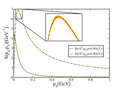
The input data for $S^{+}(p_{4},\vec{p})$ for the following example is chosen on an interval $[0\mathrm{GeV},1\mathrm{GeV}]$ for the gapped channel in the $2SC$ phase at a quark chemical potential of $\mu=1\mathrm{GeV}$. As an illustration, the input for momentum $p=0.9\mathrm{GeV}$ is shown in Fig. 1. We consider the input as continuous due to our many data points and it has small errors of less than $1\%$ in absolute value above $30\mathrm{MeV}$.

Figure 1: Real and imaginary part of the quasiparticle propagator $S^{+}$ in the gapped channel of the $2SC$ phase at a chemical potential of $\mu=1\mathrm{GeV}$ and momentum $p=0.9\mathrm{GeV}$ as a function of the Euclidean energy $p_{4}$. The errors are given as shaded regions around the lines and are of the order of their thickness.

5.3 Choice of the prior estimate

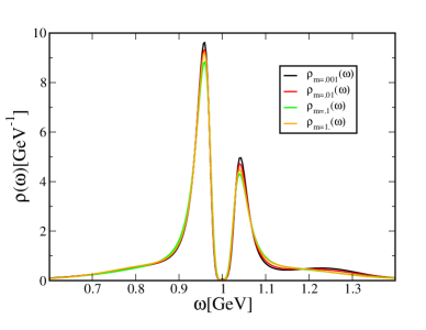
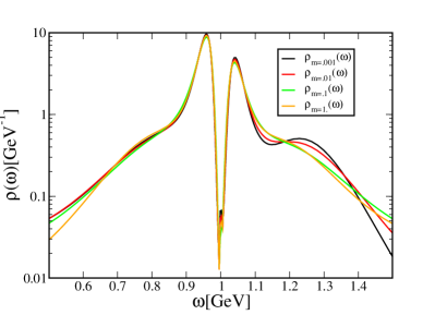
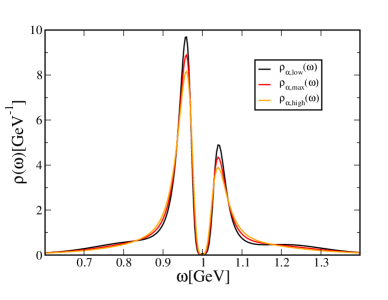
For the data input with given errors, we now need to choose an interval for the spectral function and a non-vanishing prior estimate. We take the comparatively large interval $[-1.5\mathrm{GeV},2\mathrm{GeV}]$. Furthermore we choose an interval for $P[\alpha|DH(m)]$ as discussed in the following subsection. For different prior estimates $m=0.001,0.01,0.1$ and $1.0\,\mathrm{GeV}^{-1}$ at momentum $p=0.9\mathrm{GeV}$, we then obtain the most expected spectral functions as shown in Fig. 2. It turns out, that the extracted spectral function is remarkably insensitive on the variation of the prior estimate, even when varying it by more than three orders of magnitude. This is mainly related to the small errors of our data. We therefore fix $m=0.1\mathrm{GeV}^{-1}$ in the following.

Figure 2: The most expected spectral function $\rho^{+}(\omega)$ in the gapped channel of the $2SC$ phase at momentum $p=0.9\mathrm{GeV}$ for constant prior estimates $m=0.001,0.01,0.1$ and $1.0\,\mathrm{GeV}^{-1}$ in linear (left) and logarithmic (right) presentation.

5.4 The $\alpha$-dependence

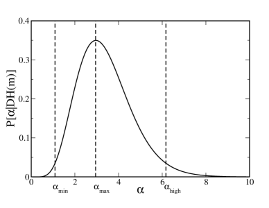
It is also interesting to investigate the $\alpha$-dependence of the maximum of the functional $Q[\rho]$ as well as of $P[\alpha|DH(m)]$. Since $P[\alpha|DH(m)]$ shows a pronounced maximum at $\alpha_{max}$, we choose the interval $I=[\alpha_{low},\alpha_{high}]$ for $P[\alpha|DH(m)]$ to be non-vanishing and normalized, such that $P[\alpha|DH(m)]>10^{-1}\times P[\alpha_{max}|DH(m)]$ for $\alpha\in I$.

Again, for momentum $p=0.9\mathrm{GeV}$, the results are shown in Fig. 3. On the left-hand side, we show $P[\alpha|DH(m)]$, normalized on $I$. On the right-hand side, we present the maximum of $Q[\rho]$ for $\alpha=\alpha_{min},\alpha_{max}$ and $\alpha_{high}$. They are only weakly varying, even when comparing the border of the interval $I$ to the maximum. This also substantiates Laplace’s rule for $P[\alpha|H(m)]$ a posteriori, assuming that its $\alpha$-dependence is weaker.

Apart from this, in Fig. 3, the most expected spectral function is equal to the most probable spectral function given at $\alpha_{max}$ and therefore not shown. Thus the “classic maximum entropy” gives very similar results as “Bryan’s method” in our case of “many” data points and small errors.

Figure 3: The function $P[\alpha|DH(m)]$ normalized between $\alpha_{min}$ and $\alpha_{high}$ (see text) with maximum $\alpha_{max}$ (left) and the maxima $\rho_{\alpha,low/max/high}$ of the functional $Q[\rho]$ for given $\alpha$ (right). Both for the gapped channel of the $2SC$ phase at momentum $p=0.9\mathrm{GeV}$.

5.5 Error estimate and final result

Finally we are able to perform an error estimation around the expected value of a given interval. Since we have two pronounced peaks for quasiparticles and quasiparticle-holes in the spectral function, we choose the intervals associated to their full width at half maximum (FWHM). The result for momentum $p=0.9\mathrm{GeV}$ is shown on the right in Fig. 4. Again, the errors turn out to be very small.

On the left-hand side we show a contour plot of the spectral density as a function of the energy $\omega$ and momentum $p$. The light (online yellow) line shows the maxima of the quasiparticle and quasiparticle-hole branches. For fixed momentum $p$, the difference between the dark (online blue) lines below and above the light (online yellow) line gives the FWHM of the corresponding peak. The latter is neglected in BCS-type spectral functions as given in Eq. (38).

Figure 4: A contour plot of most expected spectral density of the gapped $2SC$ phase at $\mu=1\mathrm{GeV}$ as described in the text (left) and the spectral function for momentum $p=0.9\mathrm{GeV}$ with the expectation value within the FWHM and its error estimate as shaded background (right).

6 Summary and conclusions

In this paper we have outlined, how the MEM can be adapted to numerical Dyson-Schwinger studies, in particular to fermions. It turns out, that the extracted spectral functions are much more reliable and stable against variation, than in applications of the MEM in lattice QCD. Reasons for this are the comparatively small errors on the input functions and the almost arbitrary large number of data points. Comparing however to the systematic error, coming from necessary truncations in Dyson-Schwinger studies, this error is negligible. Therefore this method can be useful for further applications in mesons or diquarks investigations, since currently all calculations have to be extended to complex momenta (see [13, 14]). Avoiding this and reducing the numerical effort drastically, the MEM might help to improve or extent known truncation schemes.

References

- [1] R. Alkofer and L. von Smekal, Phys. Rept. 353, 281 (2001) [arXiv:hep-ph/0007355].
- [2] C. D. Roberts and S. M. Schmidt, Prog. Part. Nucl. Phys. 45, S1 (2000) [arXiv:nucl-th/0005064].
- [3] C. S. Fischer, J. Phys. G 32, R253 (2006) [arXiv:hep-ph/0605173].
- [4] M. Jarrell, J. E. Gubernatis, Phys. Rep. 269, 133 (1996).
- [5] M. Asakawa, T. Hatsuda and Y. Nakahara, Prog. Part. Nucl. Phys. 46, 459 (2001) [arXiv:hep-lat/0011040].
- [6] F. Karsch et. al., Phys. Lett. B 530, 147 (2002) [arXiv:hep-lat/0110208]; S. Datta et. al., Phys. Rev. D 69, 094507 (2004) [arXiv:hep-lat/0312037].
- [7] W. H. Press et. al., Numerical Recipes in C, (Cambridge Univ. Press, Cambridge, 1992).
- [8] J. Skilling, in Maximum Entropy and Bayesian Methods edited by J. Skilling (Kluwer Academic Publishers, Dordrecht, 1989), p. 45.
- [9] S. F. Gull, in Maximum Entropy and Bayesian Methods edited by J. Skilling (Kluwer Academic Publishers, Dordrecht, 1989), p. 53.
- [10] R. K. Bryan, Eur. Biophys. J. 18, 165 (1990).
- [11] M. Le Bellac, Thermal Field Theory, (Cambridge Univ. Press, Cambridge, 1996).
- [12] D. Nickel, J. Wambach and R. Alkofer, Phys. Rev. D 73, 114028 (2006) [arXiv:hep-ph/0603163].
- [13] R. Alkofer, P. Watson and H. Weigel, Phys. Rev. D 65, 094026 (2002) [arXiv:hep-ph/0202053].
- [14] R. Alkofer, W. Detmold, C. S. Fischer and P. Maris, Phys. Rev. D 70, 014014 (2004) [arXiv:hep-ph/0309077].