May 2006

We consider modifications of the standard non-linear QCD evolution in an attempt to account for some of the missing ingredients discussed recently, such as correlations, discreteness in gluon emission and Pomeron loops. The evolution is numerically performed using the Balitsky-Kovchegov equation on individual configurations defined by a given initial value of the saturation scale, for reduced rapidities $y=(\alpha_{s}N_{c}/\pi)\,Y<10$. We consider the effects of averaging over configurations as a way to implement correlations, using three types of Gaussian averaging around a mean saturation scale. Further, we heuristically mimic discreteness in gluon emission by considering a modified evolution in which the tails of the gluon distributions are cut-off. The approach to scaling and the behavior of the saturation scale with rapidity in these modified evolutions are studied and compared with the standard mean-field results. For the large but finite values of rapidity explored, no strong quantitative difference in scaling for transverse momenta around the saturation scale is observed. At larger transverse momenta, the influence of the modifications in the evolution seems most noticeable in the first steps of the evolution. No influence on the rapidity behavior of the saturation scale due to the averaging procedure is found. In the cut-off evolution the rapidity evolution of the saturation scale is slowed down and strongly depends on the value of the cut-off. Our results stress the need to go beyond simple modifications of evolution by developing proper theoretical tools that implement such recently discussed ingredients.

1 Introduction

The B-JIMWLK  equations, derived over the last decade as a result of the concerted effort of several groups [1, 2, 3, 4, 5, 6, 7, 8, 10, 9, 11, 12, 13, 14, 15], build upon the original ideas on gluon saturation set out in [16] to provide the contemporary description of the evolution of QCD scattering amplitudes at high energy. Unfortunately, these are complicated equations and their complete solution is unknown. A combination of numerical [17, 18, 19, 20, 21, 22, 23, 24, 25] and analytical [26, 27, 28, 29, 30, 31, 32] studies has established the asymptotic properties of the B-JIMWLK equations. Most of these studies have focused on the mean field limit of the equations, where the B-JIMWLK set reduces to a single closed equation [12, 33] - the Balitsky-Kovchegov (BK) equation. Nevertheless, the results obtained for the BK equation are known to deviate at the most $\sim 10$% from those obtained numerically for the full B-JIMWLK [25].

In obtaining this set of equations, the gluonic density in the target was assumed to be large, and the projectile was taken as a dilute object. The strict validity of the resulting evolution scheme is, therefore, restricted to this physical domain. Further, it has become clear that the physical region of interest - i.e. that within reach of accelerators that are currently operating and those that will be operational in the near future - lies within the pre-asymptotic region of the evolution and that in this region the evolution is dominated by the, as yet poorly understood, initial conditions [34, 24, 35].

In the last two years, there has been a spurt of activity in this domain triggered by the crucial observation that important effects for the evolution are absent from the currently available evolution scheme [36, 37, 38, 39]. These new contributions stem from the understanding of the importance of gluon fluctuations and have been variably referred to as ’Pomeron loops’ [39, 42, 40, 41, 43, 44, 45, 46], ’fluctuations’ [38] or ’wave function saturation effects’. A particularly important development has been the finding of a duality transformation connecting the high and low density regimes [45, 46]. This duality places strict constraints on the form of the evolution kernel in the intermediate region. Nonetheless, the evolution in this intermediate domain is not completely understood.

Until now all analysis of the effect of these new ingredients have been addressed, both analytically and numerically, through the analogy of high-energy QCD evolution to a reaction-diffusion process [38]. These discussions are based on the study of the stochastic Fisher-Kolmogorov-Petrovsky-Piscounov (sFKPP) equation [39, 42, 47, 48, 49, 50]. The main conclusions extracted from these studies are: i) at small rapidities, mean field evolution through the BK equation remains approximately valid, but the rapidity evolution of the saturation scale is slowed down and the domain of geometric scaling is restricted, in comparison with the results of pure BK evolution; ii) at large rapidities, geometric scaling is destroyed, being replaced by a new type of scaling, sometimes referred to as diffusive [51].

At this stage, and while efforts towards the derivation of the complete evolution take place, it appears possible to attempt to implement some of the effects as effective modifications of the BK equation, and to examine whether the results agree qualitatively or not with our current knowledge and expectations from the results of the, previously mentioned, full high-energy QCD evolution. In this paper, we assess the impact of some of the proposed new contributions. In particular, we address the effect of correlations by introducing an averaging procedure for the initial conditions for the evolution. Further, we model possible effects due to the discreteness in gluon emission by considering the BK evolution of gluon distributions with cut-off tails.

The paper is organized as follows. In Section 2 we outline the numerical method used to implement the BK equation, and the procedures adopted to introduce modifications in the evolution intended to mimic the effects of correlations and gluon discreteness. Our results are presented in Section 3 and discussed in Section 4.

2 Numerical method

Non-linear QCD evolution is implemented using the BK equation [12, 33] in momentum space in the local approximation (i.e. neglecting the impact parameter dependence). This approximation should be valid for a large nucleus in the region far from its periphery. The evolved object is the unintegrated gluon distribution $\phi(k,b)\equiv\phi(k)$ with $k$ the transverse momentum, $b$ the impact parameter and where the dependence on rapidity $Y$ is implicitly understood. The unintegrated gluon distribution is related to the scattering probability of a $q\bar{q}$ dipole of transverse size $r$ on a hadronic target, $N(r,b)\equiv N(r)$, through

$$\phi(k)=\int{d^{2}r\over 2\pi r^{2}}\,e^{-ik\cdot r}N(r).$$ (1)

For the azimuthally independent piece of the solution, which gives the dominant contribution at large rapidities, the BK equation reads

$${\partial\phi(k)\over\partial y}=\int{dk^{\prime 2}\over k^{\prime 2}}\left[{k^{\prime 2}\phi(k^{\prime})-k^{2}\phi(k)\over\left|k^{\prime 2}-k^{2}\right|}+{k^{2}\phi(k)\over\sqrt{4k^{\prime 4}+k^{4}}}\right]-\phi(k)^{2},$$ (2)

with the reduced rapidity $y=(\alpha_{s}N_{c}/\pi)\,Y$. In this equation $\alpha_{s}$ is fixed. For $\alpha_{s}=0.2$, the maximum $y=10$ considered in this paper corresponds to large physical rapidities $Y\sim 50$.

The equation is solved using a 4th-order Runge-Kutta algorithm with step $\Delta y=0.025$. The integral is evaluated in the domain $-15<\ln{k}<35$ using a Gauss-Chebyshev quadrature with 400 points. Henceforth units of transverse momenta will be GeV, with the units corresponding to other quantities to be read from the respective equations. By varying the integration limits, the number of points, the step $\Delta y$, and by comparison with previous algorithms [17, 19, 23], the accuracy of the computations can be estimated to be better than 1 % in a wide region excluding one order of magnitude from the limits of the domain. It is usually much better than that. The size of this domain allows us to safely study the evolution up to $y=10$.

2.1 Initial conditions

We will use Eq. (2) to evolve individual configurations at initial rapidity $y=0$, characterized by some functional form and by a given value of the saturation scale $Q_{s0}\equiv Q_{s}(y=0)$. The first functional form (GBW) essayed is motivated by the Golec-Biernat-Wüsthoff model [52],

$$\phi_{GBW}(k)=-{1\over 2}\ {\rm Ei}\left({k^{2}\over Q_{s0}^{2}}\right),$$ (3)

with Ei the exponential-integral function. The second functional form (MF) reads

$$\phi_{MF}(k)=\gamma_{E}+\Gamma(0,\xi)+\ln{\xi},\ \ \xi=\left(Q_{s0}^{2}\over k^{2}\right)^{\delta},$$ (4)

with $\gamma_{E}$ the Euler constant and $\Gamma$ the incomplete gamma function. This form is motivated by phenomenological studies of geometric scaling in $\gamma^{*}$-nucleon and nucleus collisions [34]. It behaves $\propto\xi$ ($\ln{\xi}$) for $k\gg(\ll)Q_{s0}$. The parameter $\delta$ in this functional form acts as one minus the anomalous dimension governing the behavior of $\phi$ for large $k$. We take  $\delta=1$.

Values of the saturation scale in the region $10^{-2}\leq Q_{s0}^{2}\leq 10^{2}$ have been explored for both initial conditions. This region defines our averaging domain and has been sampled in 284 points which are roughly equidistant in logarithmic scale.

2.2 Averaging procedure and cut-off

After evolving up to a given rapidity $y$, we compute the average of $\phi(k)$ as proposed in [53] i.e.

$$\langle\phi(k)\rangle_{y}={\int_{10^{-2}}^{10^{2}}dQ_{s0}^{2}W(Q_{s0}^{2})\phi(k)\over\int_{10^{-2}}^{10^{2}}dQ_{s0}^{2}W(Q_{s0}^{2})}$$ (5)

is performed. Two different averaging procedures have been considered: the linear averaging [53]

$$W_{1}(Q_{s0}^{2})=\exp{\left[-{(Q_{s0}^{2}-\langle Q_{s0}^{2}\rangle)^{2}\over\Delta}\right]}$$ (6)

and a logarithmic averaging procedure given by

$$W_{2}(Q_{s0}^{2})={1\over Q_{s0}^{2}}\,\exp{\left[-{(\ln{Q_{s0}^{2}}-\ln\langle Q_{s0}^{2}\rangle)^{2}\over\Delta_{l}}\right]},$$ (7)

with $\langle Q_{s0}^{2}\rangle=1$. Values of $\Delta,\Delta_{l}=0.01$, 0.1, 1, 10 and 100 have been explored. Let us note that for both for the linear and the logarithmic case, $\Delta,\Delta_{l}=0.01$ is almost equivalent to a $\delta$-function, while for $\Delta,\Delta_{l}=100$ roughly 50 % of the normalization of the function is contained in the region we study, $10^{-2}\leq Q_{s0}^{2}\leq 10^{2}$. Finally, $W_{2}$ with $\Delta_{l}=100$ is essentially a flat function, with a variation $\sim 20$ % in the considered region - thus it is our model case for a wide averaging. Let us also indicate that although the practical relevance of such large values of $\Delta,\Delta_{l}$ may be questionable, our aim in this paper is to examine whether such a modification of standard BK evolution has any effect or not - thus our attitude of taking extreme values of the parameters characterizing the width of the weight functions for the averaging.

Finally, motivated by the results obtained in the framework of the sFKPP equation [38, 39, 42, 47, 48, 49, 50] which indicate that at large rapidities the dispersion of a set of initial conditions becomes linearly dependent on the rapidity, we will examine the effects of a logarithmic averaging procedure $W_{2}(Q_{s0}^{2})$ but with a rapidity dependent value of the dispersion $\Delta_{l}=y$. Again, the choice of this value is motivated not by phenomenological considerations but by the requirements of visibility of the proposed modification in our limited space of sampled initial configurations, see below.

On the other hand, and following the suggestion about the discreteness of the evolution in [38], see also [47, 48], we have introduced what we call a cut-off evolution: at every step in the evolution in Eq. (2), values of $\phi(k)<\kappa$ in the r.h.s. of this equation have been set to 0:

$${\partial\phi(k)\over\partial y} = \int{dk^{\prime 2}\over k^{\prime 2}}\left[{k^{\prime 2}\phi(k^{\prime})\theta[\phi(k^{\prime})-\kappa]-k^{2}\phi(k)\theta[\phi(k)-\kappa]\over\left|k^{\prime 2}-k^{2}\right|}+{k^{2}\phi(k)\theta[\phi(k)-\kappa]\over\sqrt{4k^{\prime 4}+k^{4}}}\right]$$ (8)

$$- \phi(k)^{2}\theta[\phi(k)-\kappa],$$

with $\theta[x]$ the step function. Values of the cut-off $\kappa=0.002$, 0.01 and 0.05 have been used, for evolution starting from a given initial condition with $Q_{s0}=\langle Q_{s0}\rangle=1$. In principle, such cut-off is proportional to the inverse of the coupling constant, but with an unknown proportionality constant which prevents us from making such connection with the value of $\alpha_{s}$ in the definition of $y$.

3 Results

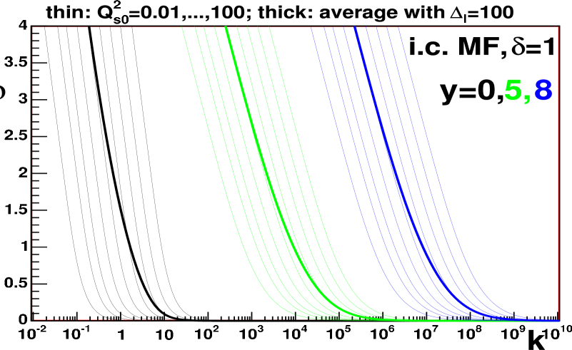
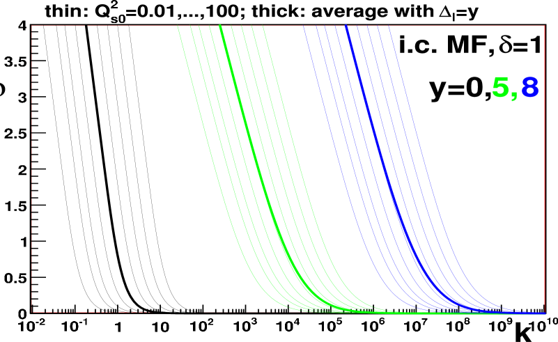
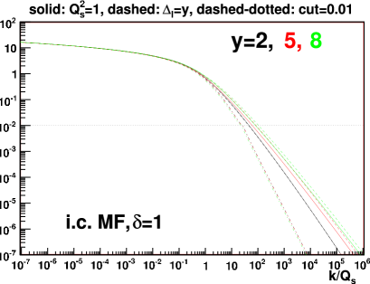
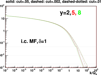
We have performed the evolution (2) starting from the initial conditions indicated in Subsection 2.1. In Fig. 1 the evolution for both initial conditions GBW and MF, for 9 given individual configurations with $Q_{s0}^{2}=0.01$, 0.04, 0.1, 0.31, 1, 3.31, 10, 30 and 100, for linear and logarithmic averages, and for the cut-off evolution, are shown. The development of traveling waves [30] can be seen in all cases and for both initial conditions. For this reason, hereon we will present results only for MF, the results for GBW being in agreement.

Figure 1: BK evolution starting from GBW (upper-left plot) and MF (the other four plots) initial conditions, all for individual configurations with $Q_{s0}^{2}=0.01$, 0.04, 0.1, 0.31, 1, 3.31, 10, 30 and 100 (thin lines left to right), for linear ($\Delta=100$, upper plots) and logarithmic averages ($\Delta_{l}=100$, middle-left plot, and $\Delta_{l}=y$, middle-right plot) using thick lines, and for cut-off evolution (thin lines, lower plot) for $\kappa=0.05$, 0.01 and 0.002 (left to right). In this last plot, horizontal dotted lines indicate the values of $\kappa$. Results are shown for $y=0$, 2, 5 and 8 in black, red, green and blue respectively (sets of lines from left to right).

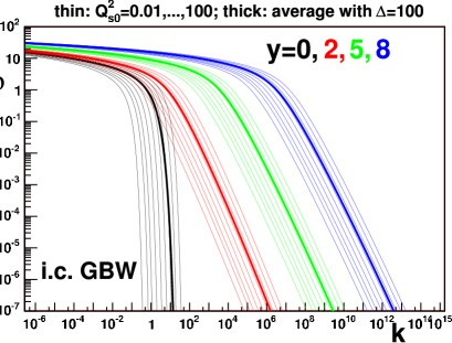
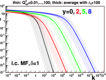
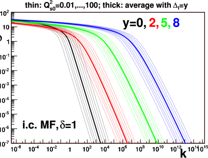
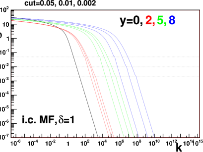
In these plots no dramatic effect of the averaging can be observed, the large-$k$ behavior appearing very similar to that of the individual configurations. This fact could be expected from the power-like behavior of the solutions of BK [27, 28, 30, 23] at large $k$. In order to see the details of the effect of the averaging we show in Fig. 2 zoomed versions of Fig. 1 in linear vertical scale. The pictures clearly show the mixing of individual configurations attained by the averaging procedure, substantiating for BK evolution the picture in [38]. It can also be seen that the effect of the averaging with a fixed dispersion is more evident in the initial condition and becomes less evident with increasing rapidities, in disagreement with present expectations from the sFKPP equation as commented previously (see e.g. [51]), while for a dispersion linearly dependent on $y$, the effect becomes, in agreement with sFKPP predictions, more and more evident with increasing rapidities.

In the next two Subsections we will examine in more detail two features of evolution, namely the approach to a universal scaling form and the evolution of the saturation scale with rapidity.

Figure 2: Details of Fig. 1 (middle-left, upper plot here, and middle-right, lower plot here) in vertical linear scale. Results for $y=2$ overlap with those for $y=0$ and are not shown for reasons of clarity.

3.1 Approach to scaling

BK evolution is known [19, 21, 23, 27, 30] to approach asymptotically a scaling function, $\phi(y,k)\to\phi(k/Q_{s}(y))$ for $y\to\infty$, independent of the initial condition for evolution. On the other hand, attempts [37, 38] to go beyond the mean field approximation underlying the BK equation predict a violation of the scaling behavior, leading to what has been called diffusive scaling [51]. Here we try to explore this aspect within our framework of modified BK evolution. For the function $\phi$ or the average of individual configurations, obtained by evolution up to a given $y$, we compute the saturation scale as the position of the maximum of the function $h(k)=k^{2}\nabla_{k}^{2}\phi(k)$, in line with previous works [17, 19, 23]. In standard BK evolution, this function shows a Gaussian-like shape which is preserved in the evolution, and the velocity of the evolution with $y$ of this soliton-like form is given by the saturation scale.

In Fig. 3 we show the results for evolution of function $\phi$ when plotted versus $k/Q_{s}(y)$. Curves for an individual configuration with $Q_{s0}=1$, and for linear and logarithmic averages and for cut-off evolution, are shown. The violation of scaling due to averaging does not look dramatic, the scaling curves being relatively close and getting closer for increasing rapidities. Only the very wide logarithmic averages seem to induce some visible violation of scaling, see below. On the other hand, scaling is achieved very quickly in the cut-off evolution (only for the largest cut-off and rapidity some departure is visible). This fact could be expected as it is known [27, 30, 24] that violations of scaling come from the tails of large $k$, which are cut in the cut-off evolution.

Figure 3: Scaling forms $\phi(k/Q_{s}(y))$ for evolution starting from MF initial conditions, for $y=2$, 5 and 8 (black, red and green lines respectively). Upper-left plot: results of an individual configuration with $Q_{s0}=1$ (solid lines), of linear ($\Delta=100$, dashed lines) averaging and with cut-off ($\kappa=0.01$, dashed-dotted lines). Upper-right plot: idem but for logarithmic ($\Delta_{l}=100$) averaging. Lower-left plot: idem but for logarithmic ($\Delta_{l}=y$) averaging. Lower-right plot: comparison of the scaling forms for different cut-offs $\kappa=0.05$ (solid lines), 0.01 (dashed lines) and 0.002 (dashed-dotted lines). In this last plot, horizontal dotted lines indicate the values of $\kappa$.

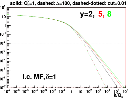
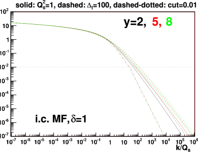
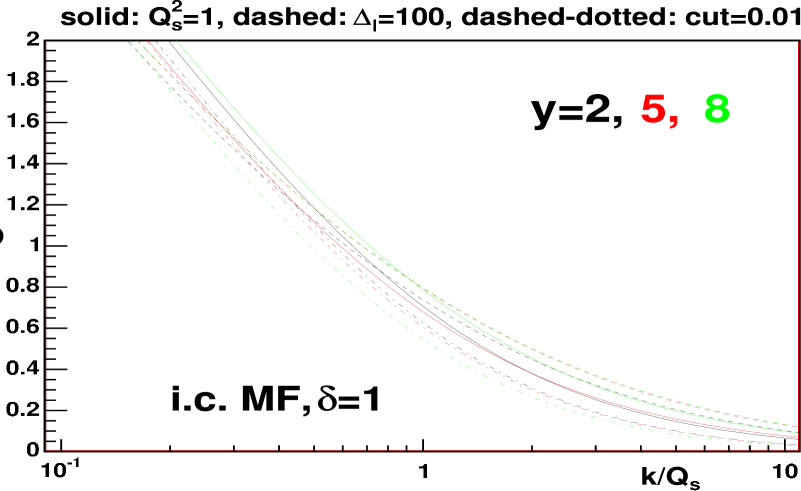
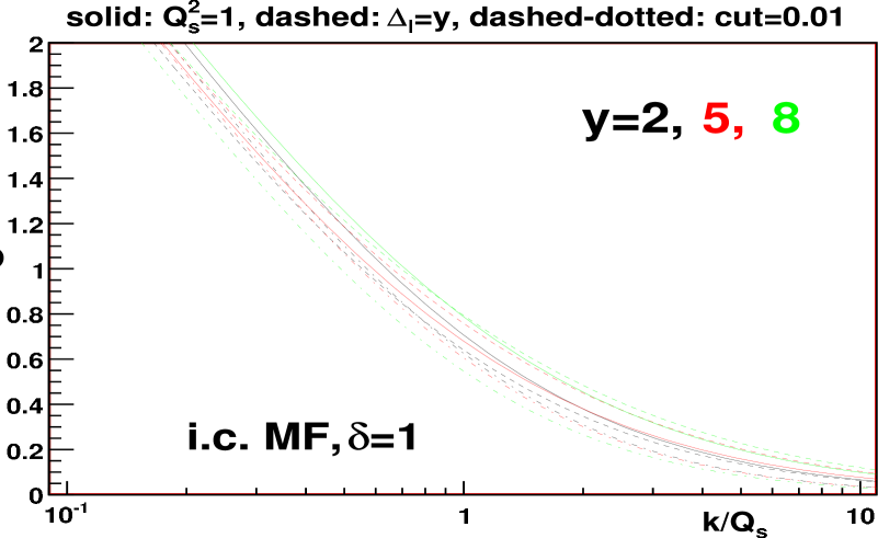
To analyze in more detail the effect of averaging on scaling, in Fig. 4 zoomed versions in linear scale of the Fig. 3 for the logarithmic averages are shown. It is well known from standard BK evolution [19, 21, 23, 27, 30] that individual configurations tend towards a universal scaling shape for the largest $y$, but violations of scaling of order $\sim 10$ % around $Q_{s}$ persist until large rapidities $y\sim 10$ [23]. The cut-off evolution shows some scaling violation, smaller than the standard BK results, and which tends to disappear with increasing $k/Q_{s}(y)$, see comments above. Besides, the averaged solutions for $\Delta_{l}=100$ show violations of scaling similar those of the individual solutions at the same $y$. But a dispersion increasing with rapidity, $\Delta_{l}=y$, produces larger violations of scaling than the case of standard BK evolution.

At first sight it looks odd that a smaller, varying dispersion creates larger violations of scaling than a larger, fixed dispersion. This is due to the fact that we sample a limited space of initial conditions, which for a very wide averaging gets immediately saturated, thus making the effect of the averaging less noticeable. So we conclude that the effect on scaling of our cut-off evolution seems to contradict the results from sFKPP evolution (it should be noted that our cut-off is applied to an evolution performed on averages, not to the evolution of individual configurations), while the effect on scaling of our averaging procedure with a dispersion increasing with rapidity agrees qualitatively with the results from sFKPP.

Figure 4: Details of Fig. 3 (upper-right, upper plot here, and lower-left, lower plot here) in vertical linear scale, for values of $k$ around $Q_{s}(y)$.

3.2 Rapidity evolution of the saturation scale

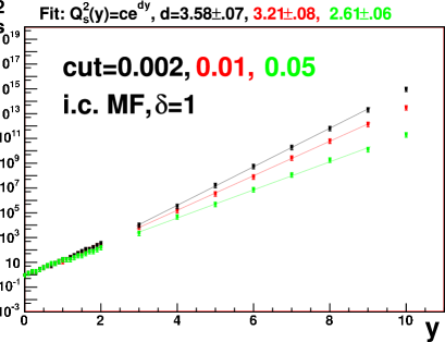
To study the rapidity evolution of the saturation scale, we determine it as indicated in the previous Subsection. An error, corresponding to the distance between neighbors in the grid at the saturation scale, is assigned to every value of the saturation scale. In Fig. 5 we show the results for the evolution of the saturation scale with reduced rapidity $y$. In order to quantify eventual differences, we have performed a fit to an exponential form $Q_{s}^{2}(y)=ce^{dy}$ in the region $3<y<9$.

Figure 5: $Q_{s}^{2}$ versus $y$ for evolution starting from MF initial conditions. In the upper and lower-left plots, the results for the evolution of individual configurations are shown for $Q_{s0}^{2}=0.01$, 1 and 100 in black, red and green respectively, while in blue the results for linear ($\Delta=100$, upper-left plot) and logarithmic ($\Delta_{l}=100$, upper-right plot, and $\Delta_{l}=y$, lower-left plot) are presented. In the lower-right plot, results of the cut-off evolution for $\kappa=0.002$ (black), 0.01 (red) and 0.05 (green) are presented. In the plots, straight lines correspond to fits to $Q_{s}^{2}(y)=ce^{dy}$ in the region $3<y<9$, with the values of $d$ indicated in the plots.

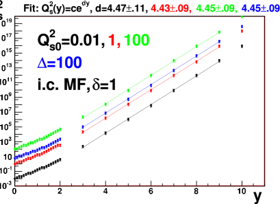
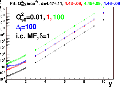
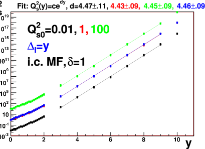
The averaging procedure shows no sizable effect, a fact which contradicts the expectations from sFKPP but can be easily understood as BK evolution is known [19, 21, 23, 27, 30] to lead asymptotically to a universal wave front moving with universal velocity (for ‘supercritical’ initial conditions, see the footnote in Subsection 2.1). Thus, asymptotically every individual configuration (even those arising from initial conditions not only with different initial saturation scale but also with different functional shape) will move with the same velocity, and the average will be characterized by this common velocity.

On the other hand, the cut-off evolution shows a strong influence on the $y$-evolution of the saturation scale in agreement with expectations from sFKPP: the larger the value of the cut-off parameter $\kappa$, the slower the evolution. This corresponds to the fact that the evolution is driven [23, 27, 30] by the large-$k$ regions, as discussed previously in Subsection 3.1.

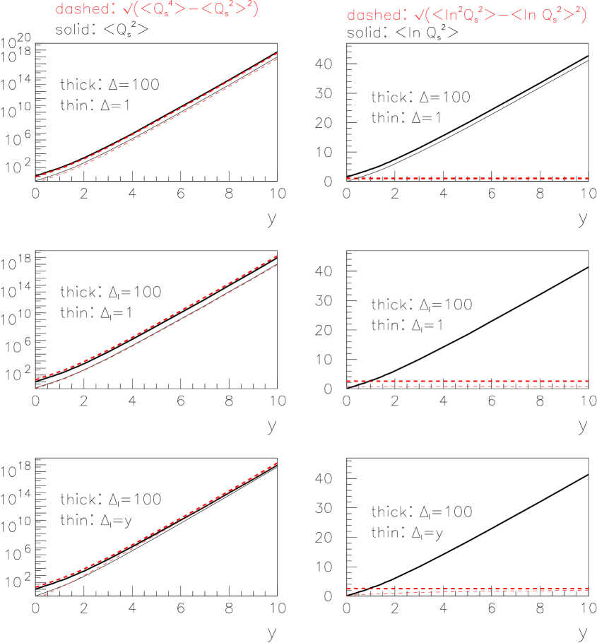
Other interesting quantity which we can examine is not the saturation scale of the averaged solution, but the average saturation scale. In the language of [30, 31, 32], the evolution of the saturation scale with rapidity shows the speed of the wave front in its movement towards higher transverse momenta. Thus the dispersion of the saturation scale at a given rapidity will reflect the spread of the ensemble of wave fronts coming through evolution from a given ensemble of initial conditions. It is then a very good quantity to characterize the effect of the evolution on a possible transition from geometric to diffusive scaling [51].

We define the average of any observable $\langle{\cal O}(y)\rangle$ by substituting $\phi(k)$ by ${\cal O}(y)$ in Eq. (5). In Fig. 6 we plot the average values $\langle Q_{s}^{2}(y)\rangle$ and $\langle\ln Q_{s}^{2}(y)\rangle$ and the corresponding dispersions, versus rapidity, for linear and logarithmic weight functions, for two different fixed values of $\Delta,\Delta_{l}$, and also for $\Delta_{l}=y$. In the case of fixed $\Delta,\Delta_{l}$ both the average $Q_{s}^{2}(y)$ and its dispersion show the same dependence with $y$, so the width of the ensemble of wave fronts gets wider and wider with increasing rapidity. On the other hand, the dispersion of $\ln Q_{s}^{2}(y)$ stays constant (within our numerical accuracy) during evolution - a behavior opposite to the linear $y$-dependence found in sFKPP [38, 48, 49, 47, 50]. Besides, smaller initial widths result in smaller widths after evolution. We expect these characteristics to remain true for large enough rapidity even if the weight functions for averaging are more involved, or even for initial ensembles containing different shapes. This is due to the fact that BK evolution eventually leads to a universal shape which, once roughly built, will evolve with the characteristics we have discussed. On the other hand, for $\Delta_{l}=y$ the dispersion of $\ln Q_{s}^{2}(y)$ increases with increasing rapidity roughly linearly in agreement with expectations from sFKPP, though with a coefficient smaller than expected from the dispersion introduced in the weight function.

Figure 6: $\langle Q_{s}^{2}(y)\rangle$ (black solid lines in the plots on the left), $\langle\ln Q_{s}^{2}(y)\rangle$ (black solid lines in the plots on the right), and their corresponding dispersions (red dashed lines in the plots on the left and right respectively) versus $y$, for linear (upper plots) and Gaussian (middle and lower plots) averaging with $\Delta,\Delta_{l}=100$ (thick lines), and $\Delta=1$, $\Delta_{l}=1$ and $\Delta_{l}=y$ (thin lines in the upper, middle and lower plots respectively), for evolution starting from MF, $\delta=1$, initial conditions. The difference between thick and thin red dashed lines in the upper-right plot, and between thick and thin black solid lines in the middle- and lower-right plots, is numerically very small and hardly visible.

4 Discussion

Much theoretical effort has been directed recently to go beyond the standard JIMWLK framework to study the small-$x$ structure of hadrons: the role of correlations [36, 55, 56, 38, 53, 50], of discreteness in gluon emissions [57, 38, 58, 59] and the relevance of Pomeron loops [37, 39, 40, 41, 42, 60, 43, 44, 45, 46, 61, 62, 63, 64]. Numerical studies are just starting [25, 47, 48, 65, 59].

In this paper we contribute to this subject through an attempt to quantify numerically the relevance of two of these aspects, namely correlations through averaging [53] and discreteness of gluon emissions [38], on standard BK evolution. The averaging of individual configurations results in scaling violations, but their size around the saturation scale is not much larger than the violations already present in standard evolution at a large but finite rapidity. On the other hand, the evolution of the saturation scale with rapidity, and the large-$k$ behavior of the solutions, seem to be hardly affected. Finally, the dispersion in the saturation scale of the individual solutions increases with rapidity at least as fast as the corresponding average, indicating that the width of the ensemble of evolved solutions gets wider and wider with increasing rapidity.

The implementation of discreteness in the evolution through a cut-off does not induce any further scaling violation. On the other hand, the saturation scale evolves slower with rapidity with increasing value of the cut-off, and the solutions at large $k$ become steeper than in the standard BK evolution.

When compared with the expectations from the sFKPP equation [39, 42, 47, 48, 49, 50], we conclude than none of the proposed modifications is able to reproduce all the features found there. The implementation of a cut-off slows down the evolution in accordance with expectations, but results in a better fulfillment of scaling, at variance with sFKPP. The averaging procedure, when implemented through a dispersion increasing with rapidity, leads to ’diffusive’ wave fronts [51], but the rapidity evolution of the saturation scale is not affected, contrary to expectations.

In view of the differences among the effects of different modifications on standard BK evolution and with the results of sFKPP, of the fact that the experimentally accessible regions of rapidity are pre-asymptotic and dominated by the initial conditions [34, 24, 35], and of the additional uncertainties on the form of the averaging weight function and/or size of the cut-off, any claim on phenomenological implications of our study looks premature. Besides, our implementation of these modifications of BK evolution is simplistic, so their results could only be taken as hints of the possible effects of a proper application of such modifications. Nevertheless, we find their effects large and diverse enough to justify the further investigations, both on the analytical and on the numerical side, currently under development to rigorously develop and implement all these new ideas. Work in this direction is in progress.

Acknowledgments: We thank M. A. Braun, J. Jalilian-Marian, A. H. Mueller, K. Tuchin and U. A. Wiedemann for useful discussions. Special thanks are given to J. L. Albacete, E. Iancu, A. Kovner and M. Lublinsky for many fruitful discussions and suggestions, and a critical reading of the manuscript. N.A. acknowledges financial support of Ministerio de Educación y Ciencia of Spain under a contract Ramón y Cajal, and of CICYT of Spain under project FPA2002-01161. J.G.M. acknowledges the partial financial support from the Fundação para a Ciência e a Tecnologia of Portugal under contract SFRH/BPD/12112/2003. N.A. also thanks IST, and J.G.M. Departamento de Física de Partículas at the Universidade de Santiago de Compostela, for warm hospitality while part of this work was done.

References

- [1] L. D. McLerran and R. Venugopalan, Phys. Rev. D 49, 2233 (1994).
- [2] L. D. McLerran and R. Venugopalan, Phys. Rev. D 49, 3352 (1994).
- [3] L. D. McLerran and R. Venugopalan, Phys. Rev. D 50, 2225 (1994).
- [4] J. Jalilian-Marian, A. Kovner, L. D. McLerran and H. Weigert, Phys. Rev. D 55, 5414 (1997).
- [5] J. Jalilian-Marian, A. Kovner, A. Leonidov and H. Weigert, Phys. Rev. D 59, 014014 (1999).
- [6] J. Jalilian-Marian, A. Kovner and H. Weigert, Phys. Rev. D 59, 014015 (1999).
- [7] A. Kovner and J. G. Milhano, Phys. Rev. D 61, 014012 (2000).
- [8] A. Kovner, J. G. Milhano and H. Weigert, Phys. Rev. D 62, 114005 (2000).
- [9] E. Iancu, A. Leonidov and L. D. McLerran, Nucl. Phys. A 692, 583 (2001).
- [10] E. Iancu, A. Leonidov and L. D. McLerran, Phys. Lett. B 510, 133 (2001).
- [11] E. Ferreiro, E. Iancu, A. Leonidov and L. McLerran, Nucl. Phys. A 703, 489 (2002).
- [12] I. Balitsky, Nucl. Phys. B 463, 99 (1996).
- [13] A. H. Mueller, Phys. Lett. B 523, 243 (2001).
- [14] J. P. Blaizot, E. Iancu and H. Weigert, Nucl. Phys. A 713, 441 (2003).
- [15] H. Weigert, Nucl. Phys. A 703, 823 (2002).
- [16] L. V. Gribov, E. M. Levin and M. G. Ryskin, Phys. Rept. 100, 1 (1983).
- [17] M. Braun, Eur. Phys. J. C 16, 337 (2000).
- [18] M. A. Kimber, J. Kwiecinski and A. D. Martin, Phys. Lett. B 508, 58 (2001).
- [19] N. Armesto and M. A. Braun, Eur. Phys. J. C 20, 517 (2001).
- [20] E. Levin and M. Lublinsky, Nucl. Phys. A 696, 833 (2001).
- [21] M. Lublinsky, Eur. Phys. J. C 21, 513 (2001).
- [22] K. Golec-Biernat, L. Motyka and A. M. Stasto, Phys. Rev. D 65, 074037 (2002).
- [23] J. L. Albacete, N. Armesto, A. Kovner, C. A. Salgado and U. A. Wiedemann, Phys. Rev. Lett. 92, 082001 (2004).
- [24] J. L. Albacete, N. Armesto, J. G. Milhano, C. A. Salgado and U. A. Wiedemann, Phys. Rev. D 71, 014003 (2005).
- [25] K. Rummukainen and H. Weigert, Nucl. Phys. A 739, 183 (2004).
- [26] E. Levin and K. Tuchin, Nucl. Phys. B 573, 833 (2000).
- [27] E. Iancu, K. Itakura and L. McLerran, Nucl. Phys. A 708, 327 (2002).
- [28] A. H. Mueller and D. N. Triantafyllopoulos, Nucl. Phys. B 640, 331 (2002).
- [29] A. H. Mueller, Nucl. Phys. A 724, 223 (2003).
- [30] S. Munier and R. Peschanski, Phys. Rev. Lett. 91, 232001 (2003).
- [31] S. Munier and R. Peschanski, Phys. Rev. D 69, 034008 (2004).
- [32] S. Munier and R. Peschanski, Phys. Rev. D 70, 077503 (2004).
- [33] Y. V. Kovchegov, Phys. Rev. D 60, 034008 (1999).
- [34] N. Armesto, C. A. Salgado and U. A. Wiedemann, Phys. Rev. Lett. 94, 022002 (2005).
- [35] J. L. Albacete, N. Armesto, J. G. Milhano, C. A. Salgado and U. A. Wiedemann, Eur. Phys. J. C 43, 353 (2005).
- [36] E. Levin and M. Lublinsky, Nucl. Phys. A 730, 191 (2004).
- [37] A. H. Mueller and A. I. Shoshi, Nucl. Phys. B 692, 175 (2004).
- [38] E. Iancu, A. H. Mueller and S. Munier, Phys. Lett. B 606, 342 (2005).
- [39] E. Iancu and D. N. Triantafyllopoulos, Nucl. Phys. A 756, 419 (2005).
- [40] A. H. Mueller, A. I. Shoshi and S. M. H. Wong, Nucl. Phys. B 715, 440 (2005).
- [41] E. Levin and M. Lublinsky, Nucl. Phys. A 763, 172 (2005).
- [42] E. Iancu and D. N. Triantafyllopoulos, Phys. Lett. B 610, 253 (2005).
- [43] C. Marquet, A. H. Mueller, A. I. Shoshi and S. M. H. Wong, Nucl. Phys. A 762, 252 (2005).
- [44] A. Kovner and M. Lublinsky, Phys. Rev. D 71, 085004 (2005).
- [45] A. Kovner and M. Lublinsky, Phys. Rev. Lett. 94, 181603 (2005).
- [46] A. Kovner and M. Lublinsky, Phys. Rev. D 72, 074023 (2005).
- [47] G. Soyez, Phys. Rev. D 72, 016007 (2005).
- [48] R. Enberg, K. Golec-Biernat and S. Munier, Phys. Rev. D 72, 074021 (2005).
- [49] E. Brunet, B. Derrida, A. H. Mueller and S. Munier, arXiv:cond-mat/0512021.
- [50] C. Marquet, R. Peschanski and G. Soyez, arXiv:hep-ph/0512186.
- [51] Y. Hatta, E. Iancu, C. Marquet, G. Soyez and D. N. Triantafyllopoulos, arXiv:hep-ph/0601150.
- [52] K. Golec-Biernat and M. Wusthoff, Phys. Rev. D 59, 014017 (1999).
- [53] A. Kovner and M. Lublinsky, JHEP 0503, 001 (2005).
- [54] K. Golec-Biernat, arXiv:hep-ph/0408255.
- [55] R. A. Janik, arXiv:hep-ph/0409256.
- [56] E. Levin and M. Lublinsky, Phys. Lett. B 607, 131 (2005).
- [57] G. P. Salam, Nucl. Phys. B 461, 512 (1996).
- [58] D. Kharzeev and K. Tuchin, Phys. Lett. B 626, 147 (2005).
- [59] C. Marquet, R. Peschanski, G. Soyez and A. Bialas, Phys. Lett. B 633, 331 (2006).
- [60] J. P. Blaizot, E. Iancu, K. Itakura and D. N. Triantafyllopoulos, Phys. Lett. B 615, 221 (2005).
- [61] Y. Hatta, E. Iancu, L. McLerran and A. Stasto, Nucl. Phys. A 762, 272 (2005).
- [62] Y. Hatta, E. Iancu, L. McLerran, A. Stasto and D. N. Triantafyllopoulos, Nucl. Phys. A 764, 423 (2006).
- [63] A. I. Shoshi and B. W. Xiao, arXiv:hep-ph/0512206.
- [64] E. Iancu, G. Soyez and D. N. Triantafyllopoulos, Nucl. Phys. A 768, 194 (2006).
- [65] V. A. Abramovsky and N. V. Prikhod’ko, arXiv:hep-ph/0512343.