Neural network approach to parton distributions fitting

Abstract

We will show an application of neural networks to extract information on the structure of hadrons. A Monte Carlo over experimental data is performed to correctly reproduce data errors and correlations. A neural network is then trained on each Monte Carlo replica via a genetic algorithm. Results on the proton and deuteron structure functions, and on the nonsinglet parton distribution will be shown.

1 Introduction

The requirements of precision physics at hadron colliders have recently led to a rapid improvement in the techniques for the determination of the structure of the nucleon. Playing this game factorization is a crucial issue. Indeed, it ensures that we can extract the parton structure of the nucleon from a process with only one initial proton (say, Deep Inelastic Scattering at HERA), and then we can use this as an input for a process where two initial protons are involved (Drell-Yan at LHC). In the QCD improved parton model the DIS structure function of the nucleon can be written as

$$F_{2}(x,\,Q^{2}) = x\left[\sum_{q=1}^{n_{f}}e_{q}^{2}\,{\cal C}^{q}\otimes q_{q}(x,Q^{2})\right.$$

$$+ \left.2n_{f}\,{\cal C}^{g}\otimes g(x,Q^{2})\right]\,$$

where $Q^{2}=-q^{2}=-(k-k^{\prime})^{2}$, $x=Q^{2}/2p\cdot q$, and $p$, $k$ and $k^{\prime}$ are the momenta of the initial nucleon, the incoming lepton, and the scattered lepton respectively; ${\cal C}^{i}$ are the coefficient functions pertubatively calculable, $q_{q}(x,Q^{2})$ and $g(x,Q^{2})$ the quarks and the gluon distributions that describe the non pertubative dynamics, the so called Parton Distribution Functions (PDFs).

The extraction of a PDF from experimental data is not trivial, even if it is a well estabilished task. In order to do that we have to evolve the PDFs to the scale of data, perform the $x$-convolution, add theoretical uncertainties (resummation, nuclear corrections, higher twist, heavy quark thresholds, $\ldots$), and then deconvolute in order to have a function of $x$ at a common scale $Q^{2}$.

Recently it has been pointed out that the uncertainty associated with a PDFs set is crucial [1, 2, 3]. The uncertainty on a PDF is given by the probability density $\mathcal{P}\left[f\right]$ in the space of functions $f(x)$, that is the measure we use to perform the functional integral that gives us the expectation value

$$\left\langle\mathcal{F}\left[f(x)\right]\right\rangle=\int\mathcal{D}f\mathcal{F}\left[f(x)\right]\mathcal{P}\left[f(x)\right]\,,$$ (2)

where $\mathcal{F}\left[f\right]$ is an arbitrary function of $f(x)$. Thus, when we extract a PDF we want to determine an infinite-dimensional object (a function) from finite set of data points, and this is a mathematically ill-posed problem.

The standard approach is to choose a simple functional form with enough free parameters ($q(x,Q_{0}^{2})=x^{\alpha}(1-x)^{\beta}P(x)$), and to fit parameters by minimizing $\chi^{2}$. Some difficulties arise: errors and correlations of parameters require at least fully correlated analysis of data errors; error propagation to observables is difficult: many observables are nonlinear/nonlocal functional of parameters; theoretical bias due to choice of parametrization is difficult to assess (effects can be large if data are not precise or hardly compatible).

Here we present an alternative approach to this problem. First we will show our technique applied to the determination of the Structure Functions. This is the easiest case, since no evolution is required, but only data fitting, thus it is a good application to test the technique. Then, we will show how this approach can be extended for the determination of the PDFs.

2 Structure functions

The strategy presented in [4, 5] to address the problem of parametrizing deep inelastic structure functions $F(x,Q^{2})$ is a combination of two techniques: a Monte Carlo sampling of the experimental data and a neural network training on each data replica.

The Monte Carlo sampling of experimental data is performed generating $N_{\mathrm{rep}}$ replicas of the original $N_{\mathrm{dat}}$ experimental data,

$$F_{i}^{(\mathrm{art})(k)} = \left(1+r_{N}^{(k)}\sigma_{N}\right)\Big{[}F_{i}^{(\mathrm{exp})}+r_{i}^{s,(k)}\sigma^{stat}_{i}$$ (3)

$$+ \sum_{l=1}^{N_{sys}}r^{l,(k)}\sigma_{i}^{sys,l}\Big{]}\,,$$

where $i=1,\ldots,N_{\mathrm{dat}}$, $\,r$ are gaussian random numbers with the same correlation as the respective uncertainties, and $\sigma^{stat},\sigma^{sys},\sigma_{N}$ are the statistical, systematic and normalization errors. The number of replicas $N_{\mathrm{rep}}$ has to be large enough so that the replica sample reproduces central values, errors and correlations of the experimental data.

The second step is to train a neural network on each data replica. A neural network [6] is a highly nonlinear mapping between input and output patterns as a function of its parameters. We choose an architecture with 4 inputs ($x$, $\log x$, $Q^{2}$, $\log Q^{2}$), two hidden layers with 5 and 3 neurons respectively, and one output, $F(x,Q^{2})$. The training on each replica is performed in two steps. First, we use the Back Propagation technique to minimize

$${\chi^{2\,(k)}_{\rm diag}}=\frac{1}{N_{\mathrm{dat}}}\sum_{i=1}^{N_{\mathrm{dat}}}\frac{\left(F_{i}^{(\mathrm{art})(k)}-F_{i}^{(\mathrm{net})(k)}\right)^{2}}{(\sigma_{i}^{\it stat})^{2}}\,;$$ (4)

then, we use the Genetic Algorithm [7] to minimize

$$\chi^{2\,(k)} = \frac{1}{N_{\mathrm{dat}}}\sum_{i,j=1}^{N_{\mathrm{dat}}}\left(F_{i}^{(\mathrm{art})(k)}-F_{i}^{(\mathrm{net})(k)}\right)$$ (5)

$$\times \mathrm{cov}^{-1}_{ij}\left(F_{j}^{(\mathrm{art})(k)}-F_{j}^{(\mathrm{net})(k)}\right)\,.$$

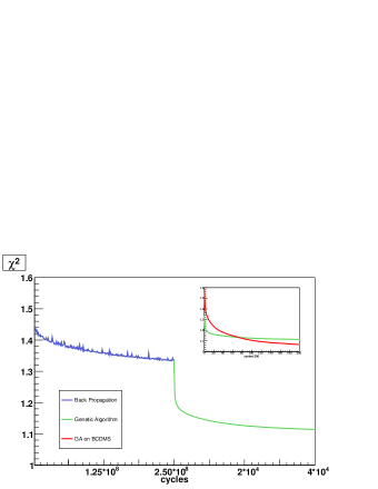
The Back Propagation technique allows for a fast minimization, but it always oscillates, while the Genetic Algorithm is always decreasing, and it is more suitable for the last part of the training where the stability of the $\chi^{2}$ is needed, see Fig. 1.

Figure 1: Dependence of the $\chi^{2}$ on the length of training: (big pad) total training (small pad), detail of the GA training.

Once we have trained all the neural networks on data replicas, we have a probability density in the space of structure functions, $\mathcal{P}\left[F(x,Q^{2})\right]$, which contains all information from experimental data, including correlations. Expectation values over this probability measure are then evaluated as averages over the trained network sample,

$$\left\langle\mathcal{F}\left[F(x,Q^{2})\right]\right\rangle=\frac{\sum_{k=1}^{N_{\mathrm{rep}}}\mathcal{F}\left(F^{(\mathrm{net})(k)}(x,Q^{2})\right)}{N_{\mathrm{rep}}}\,.$$ (6)

In Fig. 2 we show our results for the deuteron structure function $F_{2}^{d}(x,Q^{2})$ [4], and for the proton structure function $F_{2}^{p}(x,Q^{2})$ [5] compared to a polynomial parametrization [8].

Figure 2: Neural networks fit (NNPDF) compared to a polynomial fit (SMC) for the deuteron and the proton structure function.

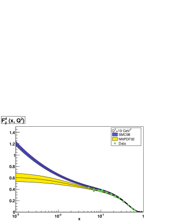
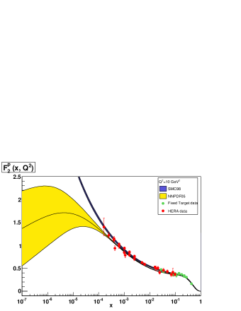
We observe that in the data range the two fits agree within errors. In the extrapolation region the error band of the polynomial fit has the same narrow width as in the data range, while the error band of the neural networks grows indicating that we are in a region where the error is underterminate since there are no data.

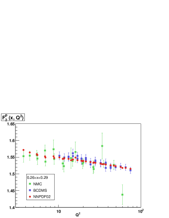
Neural networks turn to be a suitable tool also in the presence of uncompatible data. Indeed, once a good fit is obtained, say a stable value of $\chi^{2}\sim 1$, the neural networks infer a natural law by following the regularity of data, and uncompatible data are discarded without any hypotesis on the shape of the parametrization (see Fig. 3).

Figure 3: Fixed target proton data and predictions for an $x$-bin.

3 Parton distributions

The strategy presented in the above section can be used to parametrize parton distributions as well, provided one now takes into account Altarelli-Parisi QCD evolution.

Now neural networks are used to parametrize the PDF at a reference scale. We choose an architecture with 2 inputs ($x$, $\log x$), two hidden layers with 2 neurons each, and one output, $q(x,Q_{0}^{2})$. The training on each replica is performed only with the Genetic Algorithm, since we have a non local function to be minimized (see eqs. 1 and 5).

Once the fit is done, the expectation value and the error of an arbitrary function $\mathcal{F}$ of a PDF, or the correlation between different PDFs can be computed in the following way:

$$\left\langle\mathcal{F}\left[q(x)\right]\right\rangle=\frac{\sum_{k=1}^{N_{\rm rep}}\mathcal{F}\left(q^{({\rm net})(k)}(x)\right)}{N_{\rm rep}}$$

$$\sigma_{\mathcal{F}\left[q(x)\right]}=\sqrt{\left\langle\mathcal{F}\left[q(x)\right]^{2}\right\rangle-\left\langle\mathcal{F}\left[q(x)\right]\right\rangle^{2}}$$ (7)

$$\left\langle u(x_{1})d(x_{2})\right\rangle=\frac{\sum_{k=1}^{N_{\rm rep}}u^{({\rm net})(k)}(x_{1})d^{(net)(k)}(x_{2})}{N_{\rm rep}}$$

As a first application of our method, we extract the nonsinglet parton distribution $q_{NS}(x,Q^{2}_{0})=\frac{1}{6}\left(u+\bar{u}-d-\bar{d}\right)(x,Q^{2}_{0})$ from the nonsinglet structure function $F_{2}^{NS}(x,Q^{2})$ measured by the NMC [9] and BCDMS [10, 11] collaborations. The very preliminary results of a NLO fit with fully correlated uncertainties can be seen in Fig. 4 (only 25 replicas are used instead of 1000). The initial evolution scale is $Q_{0}^{2}=2\mathrm{GeV}^{2}$, and the kinematical cuts in order to avoid higher twist effects are $Q^{2}=3\,\mathrm{GeV}^{2}$ and $W^{2}=6.25\,\mathrm{GeV}^{2}$. Our result is consistent within the error bands with the results from other global fits [12, 13], but in the small-$x$ range where data are poor, differences become more sizeable. This effect will be further investigated, however, a larger number of data in the small-$x$ range for the deuteron will help in cleaning this picture.

Figure 4: Comparison of the prediction for $F_{2}^{NS}(x,Q^{2})$ with different PDF sets.

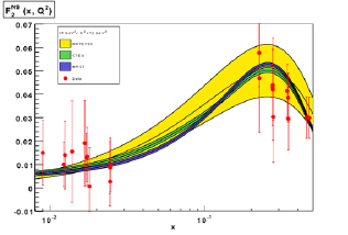
Summarizing, we have described a general technique to parametrize experimental data in an bias-free way with a faithful estimation of their uncertainties, which has been successfully applied to structure functions and that now is being implemented in the context of global parton distribution fits.

References

- [1] A. Djouadi and S. Ferrag, Phys. Lett. B 586 (2004) 345.
- [2] S. Frixione and M. L. Mangano, JHEP 0405 (2004) 056.
- [3] W. K. Tung, AIP Conf. Proc. 753 (2005) 15.
- [4] S. Forte, L. Garrido, J. I. Latorre and A. Piccione, JHEP 0205, 062 (2002).
- [5] L. Del Debbio, S. Forte, J. I. Latorre, A. Piccione and J. Rojo [NNPDF Collaboration], JHEP 0503, 080 (2005).
- [6] C. Peterson and T. Rognvaldsson, LU-TP-91-23. Lectures given at 1991 CERN School of Computing, Ystad, Sweden.
- [7] J. Rojo and J. I. Latorre, JHEP 0401 (2004) 055.
- [8] B. Adeva et al. [Spin Muon Collaboration], Phys. Rev. D 58 (1998) 112001.
- [9] M. Arneodo et al. [New Muon Collaboration], Nucl. Phys. B 483 (1997) 3.
- [10] A. C. Benvenuti et al. [BCDMS Collaboration], Phys. Lett. B 223 (1989) 485.
- [11] A. C. Benvenuti et al. [BCDMS Collaboration], Phys. Lett. B 237 (1990) 592.
- [12] A. D. Martin, R. G. Roberts, W. J. Stirling and R. S. Thorne, Eur. Phys. J. C 28 (2003) 455.
- [13] D. Stump, J. Huston, J. Pumplin, W. K. Tung, H. L. Lai, S. Kuhlmann and J. F. Owens, JHEP 0310 (2003) 046.