Study of $B\to K^{*}\rho,~{}K^{*}\omega$ Decays with Polarization in Perturbative QCD Approach

Abstract

The $B\to K^{*}\rho$, $K^{*}\omega$ decays are useful to determine the CKM angle $\phi_{3}=\gamma$. Their polarization fractions are also interesting since the polarization puzzle of the $B\to\phi K^{*}$ decay. We study these decays in the perturbative QCD approach based on $k_{T}$ factorization. After calculating of the non-factorizable and annihilation type contributions, in addition to the conventional factorizable contributions, we find that the contributions from the annihilation diagrams are crucial. They give dominant contribution to the strong phases and suppress the longitudinal polarizations. Our results agree with the current existing data. We also predict a sizable direct CP asymmetries in $B^{+}\to K^{*+}\rho^{0}$, $B^{0}\to K^{*+}\rho^{-}$, and $B^{+}\to K^{*+}\omega$ decays, which can be tested by the oncoming measurements in the B factory experiments.

PACS: 13.25.Hw, 11,10.Hi, 12,38.Bx,

1 Introduction

The hadronic $B$ decays have been studied for many years since they offer an excellent place to study the CP violation and search for new physics hints [1]. The hadronization of the final states is nonperturbative in nature, and the essential problem in handling the decay processes is the separation of different energy scales, namely, the so-called factorization assumption. Many factorization approaches have been developed to calculate the $B$ meson decays, such as the naive factorization [2], the generalized factorization [3, 4], the QCD factorization [5], as well as the perturbative QCD approach (PQCD) based on $k_{T}$ factorization [6, 7]. Most factorization approaches are based on heavy quark expansion and light-cone expansion, only the leading power or part of next to leading power contributions are calculated to compare with the experiments. Nevertheless for the penguin-dominated decay channels, the power corrections and the nonperturbative contributions may be large, since the theoretical predictions for some channels cannot fit the data quite well. There are some problems, such as the $\sin{2\beta}$ problem in penguin dominated modes [8], which suggests that more dynamics of penguin dominating B decays should be studied.

Recently, with more and more data, the B factories have measured some decays that the final state contains two vector mesons [9, 10, 11]. In the $B\to VV$ modes, both the longitudinal and the transverse polarization can contribute to the decay width, and the polarization fractions can be measured by the experiments. The naive counting rules based on the factorization approaches predict that the longitudinal polarization dominates the decay ratios and the transverse polarizations are suppressed [12] due to the helicity flips of the quark in the final state hadrons. But some data shown in table 1 are quite different from the theoretical predictions for the penguin dominated modes.

Table 1: Longitudinal Polarization fractions of some $B\to VV$ modes.

Process	Belle	Babar	QCDF [14, 24]	QCDF+FSI[17]
$B^{0}\to\phi K^{*0}$	$0.45\pm 0.05\pm 0.02$	$0.52\pm 0.05\pm 0.02$	0.91	$0.43^{+0.13}_{-0.09}$
$B^{+}\to\phi K^{*+}$	$0.52\pm 0.8\pm 0.03$	$0.46\pm 0.12\pm 0.03$	0.91	$0.43^{+0.13}_{-0.09}$
$B^{+}\to\rho^{0}K^{*+}$		$0.96^{+0.04}_{-0.15}\pm 0.04$	0.94	$0.49^{+0.11}_{-0.08}$
$B^{+}\to\rho^{+}K^{*0}$	$0.43\pm 0.11^{+0.05}_{-0.07}$	$0.79\pm 0.08\pm 0.04\pm 0.02$	0.95	$0.57^{+0.16}_{-0.14}$

The small longitudinal polarization fraction in $B\to\phi K^{\ast}$ decays has been considered as a puzzle, many theoretical efforts have been performed to explain it [13, 14, 15, 16, 17, 18, 19, 20]. In PQCD approach, the coefficients of penguin operators have been evolved to the scale of about $\sqrt{\Lambda M_{B}}$, so these coefficients become larger compared to the factorization approach, in which the hard scale are at the scale of $M_{B}$, so that the penguins’ contribution are enhanced in PQCD approach. Besides, the annihilation diagrams, which is power suppressed in QCD factorization, are also included. Thus the PQCD approach can give a larger branching ratio and fits the experiments well in $B\to PP,PV$ case. For $B\to\phi K^{\ast}$, the annihilation diagram with the $(S+P)(S-P)$ type operators will break the naive counting rules [15], the transverse polarization is enhanced to about $0.25$. But the branching ratios calculated in the PQCD approach [21] are too large if we adopt the old $K^{\ast}$ meson’s parton distribution amplitudes derived from QCD sum rules. As mentioned in [22], things will get better (59% of longitudinal polarization) if we adopt the asymptotic form of the $K^{\ast}$ meson’s parton distribution amplitudes.

In this paper, we will perform the leading order PQCD calculation of penguin dominated processes $B\to\rho K^{\ast}$ and $B\to\omega K^{\ast}$. The branching ratios have been measured by the B factories [23] which are given in table 2. And the measured CP asymmetries are: ${\cal A}_{CP}(B^{+}\to\rho^{+}K^{*0})=-0.14\pm 0.17\pm 0.4$ and ${\cal A}_{CP}(B^{+}\to\rho^{0}K^{*+})=0.20^{+0.32}_{-0.29}\pm 0.04$. These channels have been studied within the QCD factorization framework, but the predictions are not quite consistent with the data, especially the polarization fractions [24]. We hope the PQCD approach could give a better theoretical prediction.

Table 2: Branching ratios ($10^{-6}$) of $B\to\rho K^{\ast}$ measured by the B factories

Process	BaBar	Belle	world average
$B^{0}\to\rho^{-}K^{*+}$	$<24$		$<24$
$B^{+}\to\rho^{0}K^{*+}$	$10.6^{+3.0}_{-2.6}\pm 2.4$		$10.6^{+3.8}_{-3.5}$
$B^{+}\to\rho^{+}K^{*0}$	$17.0\pm 2.9^{+2.0}_{-2.8}$	$8.9\pm 1.7\pm 1.0$	$10.5\pm 1.8$
$B^{0}\to\rho^{0}K^{*0}$		$<2.6$	$<2.6$
$B^{+}\to\omega K^{*+}$	$<7.4$		$<7.4$
$B^{0}\to\omega K^{*0}$	$<6.0$		$<6.0$

The paper is organized as follows: In Sect. 2 we will present the framework for three scale PQCD factorization theorem. Next we will give the perturbative calculation result for the hard part. In Sect. 4, numerical calculation for branching ratio and CP violation are given. Final section is devoted to summary.

2 The Theoretical Framework

The PQCD factorization theorem has been developed for non-leptonic heavy meson decays [25], based on the formalism by Brodsky and Lepage [26], and Botts and Sterman [27]. In the two body hadronic $B$ decays, the $B$ meson is heavy, sitting at rest. It decays into two light mesons with large momenta. Therefore the light mesons are moving very fast in the rest frame of $B$ meson.

To form the fast moving final state light meson, in which the two valence quarks should be collinear, there must be a hard gluon to kick off the light spectator quark $d$ or $u$ in the $B$ meson (at rest). So the contribution from the hard gluon exchange between the spectator quark and the quarks which form the four quark operator dominates the matrix element of the four quark operator between hadron states. This process can be calculated perturbatively, but the endpoint singularity will appear if we drop the transverse momentum carried by the quarks. After introducing the parton’s transverse momentum, the singularity is regularized, and additional energy scale is present in the theory, then the perturbative calculation will produce large double logarithm terms, these terms are then resummed to the Sudakov form factor. The uncancelled soft and collinear divergence should be absorbed into the definition of the meson’s wave functions, then the decay amplitude is infrared safe and can be factorized as the following formalism:

$$C(t)\times H(t)\times\Phi(x)\times\exp\left[-s(P,b)-2\int_{1/b}^{t}\frac{d\bar{\mu}}{\bar{\mu}}\gamma_{q}(\alpha_{s}(\bar{\mu}))\right],$$ (1)

where $C(t)$ are the corresponding Wilson coefficients of four quark operators, $\Phi(x)$ are the meson wave functions and the variable $t$ denotes the largest energy scale of hard process $H$, it is the typical energy scale in PQCD approach and the Wilson coefficients are evolved to this scale. The exponential of $S$ function is the so-called Sudakov form factors, which can suppress the contribution from the nonperturbative region, making the perturbative region give the dominated contribution. The “$\times$” here denotes convolution, i.e., the integral on the momentum fractions and the transverse intervals of the corresponding mesons. Since logarithm corrections have been summed by renormalization group equations, the factorization above formula does not depend on the renormalization scale $\mu$ explicitly.

In the resummation procedures, the $B$ meson is treated as a heavy-light system. In general, the $B$ meson light-cone matrix element can be decomposed as [28, 5]

$$\int_{0}^{1}\frac{d^{4}z}{(2\pi)^{4}}e^{i\bf{k_{1}}\cdot z}\langle 0|\bar{b}_{\alpha}(0)d_{\beta}(z)|B(p_{B})\rangle$$ (2)

$$= -\frac{i}{\sqrt{2N_{c}}}\left\{(\not p_{B}+m_{B})\gamma_{5}\left[\phi_{B}({\bf k_{1}})-\frac{\not n_{+}-\not n_{-}}{\sqrt{2}}\bar{\phi}_{B}({\bf k_{1}})\right]\right\}_{\beta\alpha},$$

where $n_{+}=(1,0,{\bf 0_{T}})$, and $n_{-}=(0,1,{\bf 0_{T}})$ are the unit vectors pointing to the plus and minus directions, respectively. As pointed out in ref.[29], this kind of definition will provide light-cone divergence, and more involved studies have been performed [30, 31]. Here we only use it phenomenologically to fit the data, so we still use the old form. From the above equation, one can see that there are two Lorentz structures in the $B$ meson distribution amplitudes. They obey the following normalization conditions

$$\int\frac{d^{4}k_{1}}{(2\pi)^{4}}\phi_{B}({\bf k_{1}})=\frac{f_{B}}{2\sqrt{2N_{c}}},~{}~{}~{}\int\frac{d^{4}k_{1}}{(2\pi)^{4}}\bar{\phi}_{B}({\bf k_{1}})=0.$$ (3)

In general, one should consider both of these two Lorentz structures in calculations of $B$ meson decays. However, it can be argued that the contribution of $\bar{\phi}_{B}$ is numerically small [32, 33], thus its contribution can be neglected. Therefore, we only consider the contribution of Lorentz structure

$$\Phi_{B}=\frac{1}{\sqrt{2N_{c}}}(\not\!p_{B}+m_{B})\gamma_{5}\phi_{B}({\bf k_{1}}),$$ (4)

in our calculation. Note that we use the same distribution function $\phi_{B}(k_{1})$ for the $\not\!p_{B}$ term and the $m_{B}$ term in the heavy quark limit. For the hard part calculations in the next section, we use the approximation $m_{b}\simeq m_{B}$, which is the same order approximation neglecting higher twist of $(m_{B}-m_{b})/m_{B}$. Throughout this paper, we take light-cone coordinates, then the four momentum $p^{\pm}=(p^{0}\pm p^{3})/\sqrt{2}$, and ${\bf p}_{T}=(p^{1},p^{2})$. We consider the $B$ meson at rest, the momentum is $p_{B}=(m_{B}/\sqrt{2})(1,1,{\bf 0}_{T})$. The momentum of the light valence quark is written as ($k_{1}^{+},k_{1}^{-},{\bf k}_{1T}$), where the ${\bf k}_{1T}$ is a small transverse momentum. It is difficult to define the function $\phi_{B}(k_{1}^{+},k_{1}^{-},{\bf k}_{1T})$. However, the hard part isn’t always dependent on $k_{1}^{+}$ if we make some approximations. This means that $k_{1}^{+}$ can be simply integrated out for the function $\phi_{B}(k_{1}^{+},k_{1}^{-},{\bf k}_{1T})$ as

$$\phi_{B}(x,{\bf k}_{1T}) = \int dk_{1}^{+}\phi_{B}(k_{1}^{+},k_{1}^{-},{\bf k}_{1T})$$ (5)

where $x=k_{1}^{-}/p_{B}^{-}$ is the momentum fraction. Therefore, in the perturbative calculations, we do not need the information of all four momentum $k_{1}$. The integration above can be done only when the hard part of the subprocess is independent on the variable $k_{1}^{+}$.

The $K^{*}$ and $\rho$ mesons are treated as a light-light system. At the $B$ meson rest frame, they are moving very fast. We define the momentum of the $K^{*}$ as $P_{2}=(m_{B}/\sqrt{2})(1-r_{3}^{2},r_{2}^{2},{\bf 0}_{T})$. The $\rho$ has momentum $P_{3}=(m_{B}/\sqrt{2})(r_{3}^{2},1-r_{2}^{2},{\bf 0}_{T})$, with $r_{2}=M_{K^{*}}/M_{B}$ and $r_{3}=M_{\rho(\omega)}/M_{B}$. The light spectator quark in $K^{*}$ meson has a momentum $(k_{2}^{+},0,{\bf k}_{2T})$. The momentum of the other valence quark in this final meson is thus $(P_{2}^{+}-k_{2}^{+},0,-{\bf k}_{2T})$. The longitudinal polarization vectors of the $K^{*}$ and $\rho$ are given as:

$$\epsilon_{2}(L)=\frac{P_{2}}{M_{K^{*}}}-\frac{M_{K^{*}}}{P_{2}\cdot n_{-}}n_{-}\;,\epsilon_{3}(L)=\frac{P_{3}}{M_{\rho}}-\frac{M_{\rho}}{P_{3}\cdot n_{+}}n_{+}\;,\;\;\;\;$$ (6)

which satisfy the normalization $\epsilon_{2}^{2}(L)=\epsilon_{3}^{2}(L)=-1$ and the orthogonality $\epsilon_{2}(L)\cdot P_{2}=\epsilon_{3}(L)\cdot P_{3}=0$ for the on-shell conditions $P_{2}^{2}=M_{K^{*}}^{2}$ and $P_{3}^{2}=M_{\rho}^{2}$. We first keep the full dependence on the light meson masses $M_{K^{*}}$ and $M_{\rho}$ with the momenta $P_{2}$ and $P_{3}$. After deriving the factorization formulas, which are well-defined in the limit $M_{K^{*}},M_{\rho}\to 0$, we drop the terms proportional to $r^{2}_{\rho},\ r_{K^{*}}^{2}\sim 0.04$. The transverse polarization vectors can be adapted directly as

$$\epsilon(+)=\frac{1}{\sqrt{2}}(0,0,1,i)\;,\;\;\;\;\epsilon(-)=\frac{1}{\sqrt{2}}(0,0,1,-i)\;.$$ (7)

If the ${K^{*}}$ meson (so as to other vector mesons) is longitudinally polarized, we can write its wave function in longitudinal polarization [32, 34]

$$<{K^{*}}^{-}(P,\epsilon_{L})|\overline{s}_{\alpha}(z)u_{\beta}(0)|0>$$ (8)

$$= \frac{1}{\sqrt{2N_{c}}}\int_{0}^{1}dxe^{ixP\cdot z}\left\{\not\!\epsilon\left[\not\!p_{K^{*}}\phi_{K^{*}}^{t}(x)+m_{K^{*}}\phi_{K^{*}}(x)\right]+m_{K^{*}}\phi_{K^{*}}^{s}(x)\right\}.$$

The second term in the above equation is the leading twist wave function (twist-2), while the first and third terms are sub-leading twist (twist-3) wave functions. If the $K^{*}$ meson is transversely polarized, its wave function is then

$$<{K^{*}}^{-}(P,\epsilon_{T})|\overline{s}_{\alpha}(z)u_{\beta}(0)|0> = \frac{1}{\sqrt{2N_{c}}}\int_{0}^{1}dxe^{ixP\cdot z}\left\{\not\!{\epsilon}\left[\not\!p_{K^{*}}\phi_{K^{*}}^{T}(x)+m_{K^{*}}\phi_{K^{*}}^{v}(x)\right]\right.$$ (9)

$$\left.+im_{K^{*}}\epsilon_{\mu\nu\rho\sigma}\gamma_{5}\gamma^{\mu}\epsilon^{\nu}n^{\rho}v^{\sigma}\phi_{K^{*}}^{a}(x)\right\}.$$

Here the leading twist wave function for the transversely polarized $K^{*}$ meson is the first term which is proportional to $\phi_{K^{*}}^{T}$.

The transverse momentum ${\bf k}_{iT}$ is usually converted to the $b$ parameter by Fourier transformation. The initial conditions of $\phi_{i}(x),i=B,K^{*},\rho$, are of nonperturbative origin, satisfying the normalization

$$\int_{0}^{1}\phi_{i}(x,b=0)dx=\frac{1}{2\sqrt{2N_{c}}}f_{i},$$ (10)

with $f_{i}$ the meson decay constants.

3 Perturbative Calculations

With the above brief discussion, the only thing left is to compute the hard part $H$ . We use the notation $M_{\lambda}=<V_{1}(\lambda)V_{2}(\lambda)|H^{eff}_{wk}|B>$ for the helicity matrix element, $\lambda=0,\pm 1$. For decays of $B$ to two vector mesons, the amplitude can be expressed by three invariant helicity amplitudes, defined by the decomposition

$$M_{\lambda}=M^{(1)}\epsilon^{*}_{K^{*}}(\lambda)\cdot\epsilon^{*}_{\rho}(\lambda)+M^{(2)}\epsilon^{*}_{K^{*}}(\lambda)\cdot P_{\rho}\epsilon^{*}_{\rho}(\lambda)\cdot P_{K^{*}}+M^{(3)}i\varepsilon_{\mu\nu\omega\sigma}\epsilon_{K^{*}}^{*\mu}(\lambda)\epsilon_{\rho}^{*\nu}(\lambda)P^{\omega}_{K^{*}}P_{\rho}^{\sigma}.$$ (11)

According to the naive counting rules mentioned before, we can estimate that polarization fractions satisfy the relation: $|M_{0}|^{2}\gg|M_{-}|^{2}\gg|M_{+}|^{2}$. These three helicity amplitudes can be expressed as another set of helicity amplitudes,

$$M_{0}=M_{B}^{2}M_{L},~{}M_{\pm}=M_{B}^{2}M_{N}{\mp}M_{K^{*}}^{2}\sqrt{r^{\prime}-1}M_{T}$$ (12)

where the $M_{L}$, $M_{N}$ and $M_{T}$ can be extracted directly from calculation of the Feynman diagrams, and $r^{\prime}=\frac{P_{2}\cdot P_{3}}{M_{K^{*}}M_{\rho}}$. The formula for the decay width is

$$\Gamma=\frac{p}{8\pi M_{B}^{2}}\sum M_{(\sigma)}^{\dagger}M_{(\sigma)}.$$ (13)

Here $p$ is the absolute value of the 3-momentum of the final state mesons. And we have

$$\sum M_{(\sigma)}^{\dagger}M_{(\sigma)} =|M_{0}|^{2}+|M_{+}|^{2}+|M_{-}|^{2}..$$

The weak Hamiltonian ${\cal H}_{{\it eff}}$ for the $\Delta B=1$ transitions at the scale smaller than $m_{W}$ is given as [35]

$${\cal H}_{{\it eff}}=\frac{G_{F}}{\sqrt{2}}\,\left[V_{ub}V_{us}^{*}\left(C_{1}O_{1}^{u}+C_{2}O_{2}^{u}\right)-V_{tb}V_{ts}^{*}\,\left(\sum_{i=3}^{10}C_{i}\,O_{i}+C_{g}O_{g}\right)\right]\quad.$$ (14)

We specify below the operators in ${\cal H}_{{\it eff}}$ for $b\to s$:

$$\begin{array}[]{llllll}O_{1}^{u}&=&\bar{s}_{\alpha}\gamma^{\mu}Lu_{\beta}\cdot\bar{u}_{\beta}\gamma_{\mu}Lb_{\alpha}\ ,&O_{2}^{u}&=&\bar{s}_{\alpha}\gamma^{\mu}Lu_{\alpha}\cdot\bar{u}_{\beta}\gamma_{\mu}Lb_{\beta}\ ,\\ O_{3}&=&\bar{s}_{\alpha}\gamma^{\mu}Lb_{\alpha}\cdot\sum_{q^{\prime}}\bar{q}_{\beta}^{\prime}\gamma_{\mu}Lq_{\beta}^{\prime}\ ,&O_{4}&=&\bar{s}_{\alpha}\gamma^{\mu}Lb_{\beta}\cdot\sum_{q^{\prime}}\bar{q}_{\beta}^{\prime}\gamma_{\mu}Lq_{\alpha}^{\prime}\ ,\\ O_{5}&=&\bar{s}_{\alpha}\gamma^{\mu}Lb_{\alpha}\cdot\sum_{q^{\prime}}\bar{q}_{\beta}^{\prime}\gamma_{\mu}Rq_{\beta}^{\prime}\ ,&O_{6}&=&\bar{s}_{\alpha}\gamma^{\mu}Lb_{\beta}\cdot\sum_{q^{\prime}}\bar{q}_{\beta}^{\prime}\gamma_{\mu}Rq_{\alpha}^{\prime}\ ,\\ O_{7}&=&\frac{3}{2}\bar{s}_{\alpha}\gamma^{\mu}Lb_{\alpha}\cdot\sum_{q^{\prime}}e_{q^{\prime}}\bar{q}_{\beta}^{\prime}\gamma_{\mu}Rq_{\beta}^{\prime}\ ,&O_{8}&=&\frac{3}{2}\bar{s}_{\alpha}\gamma^{\mu}Lb_{\beta}\cdot\sum_{q^{\prime}}e_{q^{\prime}}\bar{q}_{\beta}^{\prime}\gamma_{\mu}Rq_{\alpha}^{\prime}\ ,\\ O_{9}&=&\frac{3}{2}\bar{s}_{\alpha}\gamma^{\mu}Lb_{\alpha}\cdot\sum_{q^{\prime}}e_{q^{\prime}}\bar{q}_{\beta}^{\prime}\gamma_{\mu}Lq_{\beta}^{\prime}\ ,&O_{10}&=&\frac{3}{2}\bar{s}_{\alpha}\gamma^{\mu}Lb_{\beta}\cdot\sum_{q^{\prime}}e_{q^{\prime}}\bar{q}_{\beta}^{\prime}\gamma_{\mu}Lq_{\alpha}^{\prime}~{}.\end{array}$$ (15)

Here $\alpha$ and $\beta$ are the $SU(3)$ color indices; $L$ and $R$ are the left- and right-handed projection operators with $L=(1-\gamma_{5})$, $R=(1+\gamma_{5})$. The sum over $q^{\prime}$ runs over the quark fields that are active at the scale $\mu=O(m_{b})$, i.e., $(q^{\prime}\epsilon\{u,d,s,c,b\})$.

The diagrams for these decays are completely the same as ones in the decay $B\to K\pi$. Here we take the decay $B\to\rho^{0}K^{*+}$ as an example, whose diagrams are shown in Figure 1. These are all single hard gluon exchange diagrams, containing all leading order PQCD contributions. The analytic calculation is performed through the contraction of these hard diagrams and the Lorenz structures of the mesons’ wave functions. The first row and the third row in Figure 1 are called emission diagrams, with the $\rho$ meson or $K^{*}$ meson emitted. The analytic formulae for the $K^{*}$ meson emission diagram is exactly the same as the emission diagrams of $B\to K^{*+}\phi$ with $f_{\phi}\to f_{K^{*}},\,\,f_{K^{*}}\to f_{\rho}$, and we can get the formulae for the $\rho$ emission diagrams through the change $f_{\phi}\to f_{\rho},\,\,x_{3}\to x_{2}$ from $B\to K^{*+}\phi$. As to the annihilation diagrams, we make the same change as the $K^{*}$ emission diagrams for the corresponding diagrams of $B\to K^{*+}\phi$, then we can get the right analytic formulae.

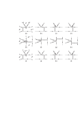
Figure 1: Diagrams contributing to the $B^{+}\to K^{*+}\rho^{0}$ decays

In PQCD approach, only Wilson coefficients are channel dependent. There are six different decay channels in $B^{+}(B^{0})\to\rho(\omega)K^{*}$ decays, and the $B^{-}\bar{(B^{0})}$ decays are their CP conjugation. All these decays are included in the twelve diagrams, the only changes needed are external quarks and the Wilson coefficients. We summarize the Wilson coefficients for each channels in table 3. In this table the coefficients are defined as

$$a_{1}=C_{1}+C_{2}/N_{c},~{}~{}~{}~{}~{}a_{2}=C_{2}+C_{1}/N_{c},$$

$$a^{q}_{3}=C^{q}_{3}+C^{q}_{4}/N_{c}+\frac{3}{2}e_{q}(C_{9}+C_{10}/N_{c}),$$

$$a^{q}_{4}=C^{q}_{4}+C^{q}_{3}/N_{c}+\frac{3}{2}e_{q}(C_{10}+C_{9}/N_{c}),$$

$$a^{q}_{5}=C^{q}_{5}+C^{q}_{6}/N_{c}+\frac{3}{2}e_{q}(C_{7}+C_{8}/N_{c}),$$

$$a^{q}_{6}=C^{q}_{6}+C^{q}_{5}/N_{c}+\frac{3}{2}e_{q}(C_{8}+C_{7}/N_{c}),$$ (16)

and

$$a^{\prime q}_{3}=C^{q}_{3}+\frac{3}{2}e_{q}C_{9},$$ (17)

$$a^{\prime q}_{4}=C^{q}_{4}+\frac{3}{2}e_{q}C_{10},$$

$$a^{\prime q}_{5}=C^{q}_{5}+\frac{3}{2}e_{q}C_{7},$$

$$a^{\prime q}_{6}=C^{q}_{6}+\frac{3}{2}e_{q}C_{8}.$$ (18)

Table 3: Wilson coefficients (the characters in the first row stand for the diagrams in figure 1 )

Process	(a)(b)	(c)(d)	(g)(h)	(e)(f)	(i)(j)	(k)(l)
$B^{0}\to\rho^{-}K^{*+}$			$a^{(d)}_{4},a^{(d)}_{6}$	$a^{\prime(d)}_{3},a^{\prime(d)}_{5}$	$a_{2},a^{(u)}_{4}$	$C_{1},a^{\prime(u)}_{3},a^{\prime(u)}_{5}$
$B^{+}\to\rho^{0}K^{*+}$	$a_{1},a^{(u-d)}_{3},a^{(u-d)}_{5}$	$C_{2},a^{\prime(u-d)}_{4},a^{\prime(u-d)}_{6}$	$a_{2},a^{(u)}_{4},a^{(u)}_{6}$	$C_{1},a^{\prime(u)}_{3},a^{\prime(u)}_{5}$	$a_{2},a^{(u)}_{4}$	$C_{1},a^{\prime(u)}_{3},a^{\prime(u)}_{5}$
$B^{+}\to\rho^{+}K^{*0}$			$a_{2},a^{(u)}_{4},a^{(u)}_{6}$	$C_{1},a^{\prime(u)}_{3},a^{\prime(u)}_{5}$	$a^{(d)}_{4}$	$a^{\prime(d)}_{3},a^{\prime(d)}_{5}$
$B^{0}\to\rho^{0}K^{*0}$	$a_{1},a^{(u-d)}_{3},a^{(u-d)}_{5}$	$C_{2},a^{\prime(u-d)}_{4},a^{\prime(u-d)}_{6}$	$a^{(d)}_{4},a^{(d)}_{6}$	$a^{\prime(d)}_{3},a^{\prime(d)}_{5}$	$a^{(d)}_{4}$	$a^{\prime(d)}_{3},a^{\prime(d)}_{5}$
$B^{0}\to\omega K^{*0}$	$a_{1},a^{(u+d)}_{3},a^{(u+d)}_{5}$	$C_{2},a^{\prime(u+d)}_{4},a^{\prime(u+d)}_{6}$	$a^{(d)}_{4},a^{(d)}_{6}$	$a^{\prime(d)}_{3},a^{\prime(d)}_{5}$	$a^{(d)}_{4}$	$a^{\prime(d)}_{3},a^{\prime(d)}_{5}$
$B^{+}\to\omega K^{*+}$	$a_{1},a^{(u+d)}_{3},a^{(u+d)}_{5}$	$C_{2},a^{\prime(u+d)}_{4},a^{\prime(u+d)}_{6}$	$a_{2},a^{(u)}_{4},a^{(u)}_{6}$	$C_{1},a^{\prime(u)}_{3},a^{\prime(u)}_{5}$	$a_{2},a^{(u)}_{4}$	$C_{1},a^{\prime(u)}_{3},a^{\prime(u)}_{5}$

4 Numerical Calculations and Discussions of Results

In the numerical calculations we use [36]

$$f_{B}=190MeV, m_{K^{*}}=0.892\mbox{ GeV}, m_{\rho}=0.77\mbox{ GeV},$$

$$M_{B}=5.28{GeV}, f_{K^{*}}=217{MeV}, f_{K^{*}}^{T}=160MeV,$$

$$M_{W}=80.41{GeV}, f_{\rho}=205{MeV}, f_{\rho}^{T}=155MeV,$$

$$m_{\omega}=0.782\mbox{ GeV}, f_{\omega}=195{MeV}, f_{\omega}^{T}=140MeV,$$

$$\tau_{B^{\pm}}=1.671\times 10^{-12}\mbox{ s,} \tau_{B^{0}}=1.536\times 10^{-12}\mbox{ s}, \Lambda_{\overline{\mathrm{MS}}}^{(f=4)}=250{MeV}.$$ (19)

The distribution amplitudes $\phi_{\rho}^{i}(x)$ ($\phi_{\omega}^{i}(x)$) and $\phi_{K^{*}}^{i}(x)$ of the light mesons used in the numerical calculation are listed in Appendix A.

For $B$ meson, the wave function is chosen as

$$\phi_{B}(x,b) = N_{B}x^{2}(1-x)^{2}\exp\left[-\frac{M_{B}^{2}\ x^{2}}{2\omega_{b}^{2}}-\frac{1}{2}(\omega_{b}b)^{2}\right],$$ (20)

with $\omega_{b}=0.4$ GeV [37], and the normalization constant $N_{B}=91.784$ GeV. We would like to point out that the choice of the meson wave functions and the parameters above is the result of a global fitting for $B\to\pi\pi$ and $B\to\pi K$ decays [6, 7].

For the CKM matrix elements, we use $|V_{us}V_{ub}^{*}|=0.00078$, $|V_{ts}V_{tb}^{*}|=0.0395$. We leave the CKM angle $\phi_{3}$ as a free parameter, which is defined as

$$V_{ub}=|V_{ub}|exp(-i\phi_{3}).$$ (21)

The decay amplitude of $B\to K^{*}\rho$ can be written as

$${\cal M}^{(i)} = V_{ub}^{*}V_{us}T^{(i)}-V_{tb}^{*}V_{ts}P^{(i)}$$ (22)

$$= V_{ub}^{*}V_{us}T^{(i)}\left[1-z^{(i)}e^{i(-\phi_{3}+\delta^{(i)})}\right],~{}~{}i=1,2,3,$$

where $z^{(i)}=\left|\frac{V_{tb}^{*}V_{ts}}{V_{ub}^{*}V_{us}}\right|\left|\frac{P^{(i)}}{T^{(i)}}\right|$, and $\delta^{(i)}$ is the relative strong phase between tree (T) diagrams and penguin diagrams (P). $z^{(i)}$ and $\delta^{(i)}$ can be calculated perturbatively. Here in PQCD approach, the strong phases come from the non-factorizable diagrams and annihilation type diagrams (see (c) $\sim$ (h) in Figure 1). The internal quarks and gluons can be on mass shell, and then poles appear in the propagators, which can provide the strong phases. The predominant contribution to the relative strong phase $\delta$ comes from the annihilation diagrams, (g) and (h) in Figure 1.

This mechanism of producing strong phase is very different from the so-called Bander-Silverman-Soni (BSS) mechanism [38], where the strong phase comes from the perturbative charm penguin diagrams. The contribution of BSS mechanism to the direct CP violation in $B\to K^{*}\rho$ is only in the higher order corrections ($\alpha_{s}$ suppressed) in our PQCD approach. Therefore we can safely neglect this contribution.

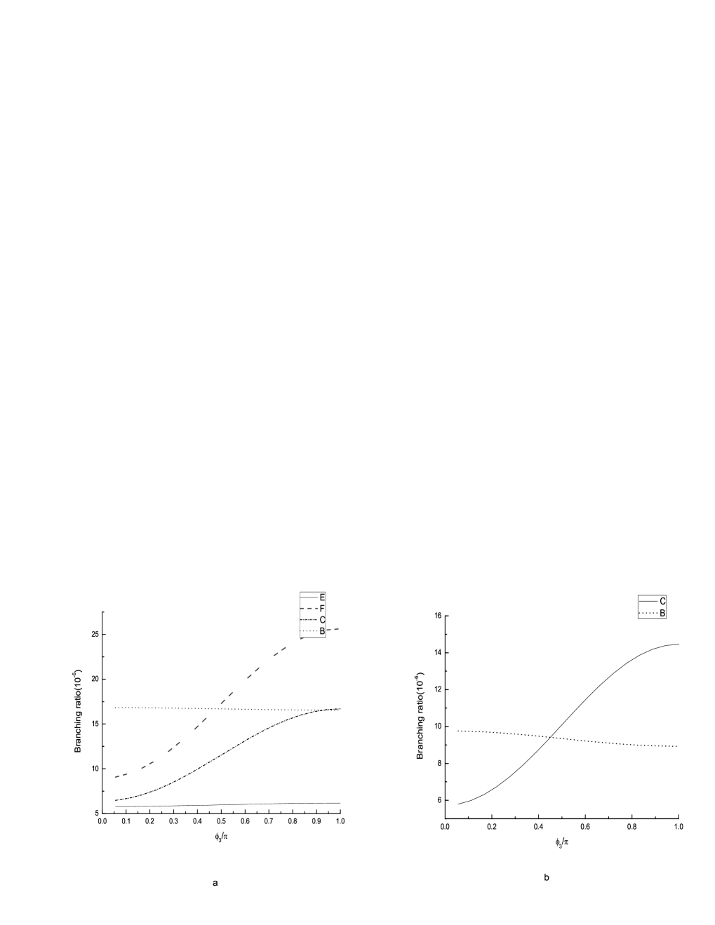
Figure 2: Averaged branching ratios ($10^{-6}$) of $B\to K^{*}\rho$ and $B\to K^{*}\omega$ as a function of CKM angle $\phi_{3}$, where the lines B,C,E,F in diagram (a) represent $B^{+}\to\rho^{+}K^{*0}$,$B^{+}\to\rho^{0}K^{*+}$, $B^{0}\to\rho^{0}K^{*0}$, $B^{0}\to\rho^{-}K^{*+}$ respectively, and in diagram (b), B denotes $B^{0}\to\omega K^{*0}$, C denotes $B^{+}\to\omega K^{*+}.$

The corresponding charge conjugate $\bar{B}$ decay is

$${\cal M}^{(i)} = V_{ub}V_{us}^{*}T^{(i)}-V_{tb}V_{ts}^{*}P^{(i)}$$ (23)

$$= V_{ub}V_{us}^{*}T^{(i)}\left[1-z^{(i)}e^{i(\phi_{3}+\delta^{(i)})}\right].$$

In contrast to the decay of $B$ to pseudoscalar mesons like $B\to K\pi$, where the decay widths can be expressed in terms of $\delta$ and $\phi_{3}$ in a simple way, here for $B$ decay to two vector mesons, there are 3 types of amplitudes, and this makes the dependence of decay widths on $\delta$ and $\phi_{3}$ very complicated. The averaged decay width for $B$ and its CP conjugation decays can be expressed as a function of a CKM phase angle $\phi_{3}$.

$$\Gamma=\frac{p}{8\pi M_{B}^{2}}|V_{ub}^{*}V_{us}|^{2}[T_{L}^{2}(1+z_{L}^{2}+2z_{L}cos\phi_{3}\cos\delta_{L})+2\sum_{i=N,T}T_{i}^{2}(1+z_{i}^{2}+2z_{i}cos\phi_{3}\cos\delta_{i})].$$ (24)

From this formula we can know that when contribution from the penguin diagrams are much larger than that from the tree diagrams, i.e., $z_{i}\gg 1,i=L,N,T$, then the branching ratios are insensitive to the angle, but when they are comparable, the dependence on $\phi_{3}$ will be strong. We show the branching ratios of these decays in Figure 2, from which we can see that the penguin dominant decays $B^{+}\to\rho^{+}K^{*0}$,$B^{0}\to\rho^{0}K^{*0}$, and $B^{0}\to\omega K^{*0}$ are almost independent on $\phi_{3}$, but the dependence on $\phi_{3}$ of the other three channels is strong, because of the tree and penguin interference.

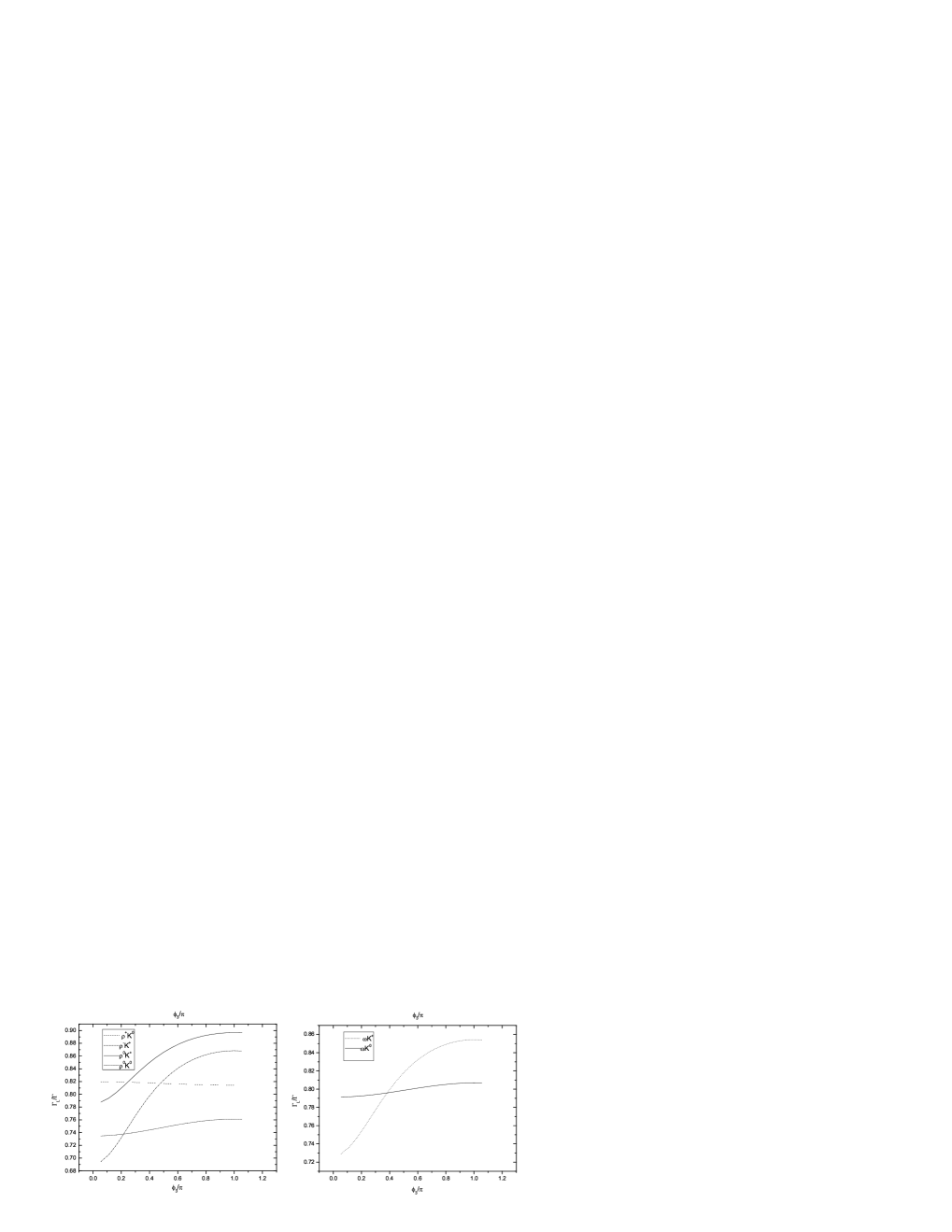
Figure 3: Longitudinal polarization fraction of $B\to K^{*}\rho$ and $B\to K^{*}\omega$ as a function of CKM angle $\phi_{3}$

In Figure 3, we plot the dependence of longitudinal polarization fractions $\Gamma_{L}/\Gamma$ on the CKM angle $\phi_{3}$. We find that this quantity is not very sensitive to $\phi_{3}$ in all decay channels. If we fix $\phi_{3}$ at about $60^{\circ}$, we find that for the decays $B^{+}\to K^{*+}\rho^{0}$ and $B^{+}\to K^{*0}\rho^{+}$, the longitudinal fractions are 0.89 and 0.82 respectively. As mentioned before, we calculate the annihilation type diagrams in PQCD approach. If the four quark operator has the Dirac structure like $(S-P)(S+P)$, there is no helicity flip suppression to the transverse polarization, so that the longitudinal fractions are considerably suppressed. One can see that our results for $B^{+}\to K^{*0}\rho^{+}$ are consistent with BaBar, but different from Belle (we hope more efforts from experimental side to test our prediction). As to $B^{+}\to K^{*+}\rho^{0}$, our result is a little smaller, but still agree with the data within the 1$\sigma$ error bar.

The new analysis of the $K^{*}$ meson wave function from QCD sum rules [39] shows that the leading twist distribution amplitude $\phi_{K^{*}}(x)$ of longitudinal polarization should be very close to the asymptotic one. According to Li’s suggestion [22], we test our result using the asymptotic wave functions for the longitudinal polarization part. The numerical results are given in table 4. We find that the longitudinal fraction and the branching ratios for all the channels are reduced. Note that Figure 2 shows that the branching ratios of $B^{o}\to K^{*0}\omega$ and $B^{+}\to K^{*+}\omega$ are larger than the experimental limits where we use the wave functions given in the appendix. But if we adopt the asymptotic form, the branching ratios decrease. Comparing the table with the experimental data, it seems that the asymptotic form is more convincing. More study of the vector meson’s wave functions are required.

Table 4: Branching ratios ($10^{-6}$) and polarization fractions using different type of light meson wave functions (the CKM phase angle $\phi_{3}$ is fixed as $60^{\circ}$; the w.f. stands for $wave\,function$)

Quantity	w.f. in the appendix	asymptotic w.f.
$Br(B^{0}\to\rho^{-}K^{*+})$	13	9.8
$Br(B^{+}\to\rho^{+}K^{*0})$	$17$	$13$
$Br(B^{+}\to\rho^{0}K^{*+})$	9.0	6.4
$Br(B^{0}\to\rho^{0}K^{*0})$	$5.9$	$4.7$
$Br(B^{+}\to\omega K^{*+})$	7.9	5.5
$Br(B^{0}\to\omega K^{*0})$	$9.6$	$6.6$
$R_{L}(B^{0}\to\rho^{-}K^{*+})$	$0.78$	$0.71$
$R_{L}(B^{+}\to\rho^{+}K^{*0})$	$0.82$	$0.76$
$R_{L}(B^{+}\to\rho^{0}K^{*+})$	$0.85$	$0.78$
$R_{L}(B^{+}\to\omega K^{*+})$	$0.81$	$0.73$
$R_{L}(B^{0}\to\rho^{0}K^{*0})$	$0.74$	$0.68$
$R_{L}(B^{0}\to\omega K^{*0})$	$0.82$	$0.74$

It has been confirmed that there is big direct CP violation in $B\to\pi K$ and $B\to\pi\pi$ decays [23], and the PQCD approach can give right predictions from the annihilation topology [40] rather than the BSS mechanism. Here we take the definition (note that our definition has opposite sign when comparing with the definition used in [23])

$$A_{CP}=\frac{\Gamma(B\to f)-\Gamma(\bar{B}\to\bar{f})}{\Gamma(B\to f)+\Gamma(\bar{B}\to\bar{f})}.$$ (25)

The direct CP violation parameters as a function of $\phi_{3}$ are shown in Figure 4. Since CP asymmetry is sensitive to many parameters, the line should be broadened by uncertainties. The direct CP violation parameter of $B^{+}\to K^{*+}\rho^{0}$, $B^{0}\to K^{*+}\rho^{-}$ and $B^{+}\to K^{*+}\omega$ can be large as $15-20\%$ when $\phi_{3}$ is near $60^{\circ}$, but for $B^{+}\to K^{*0}\rho^{+}$, the direct CP violation is very small for the very tiny tree diagram contribution. The final state is not the CP eigenstate, so the mixing induced CP violation is more complicated, and we do not give it here.

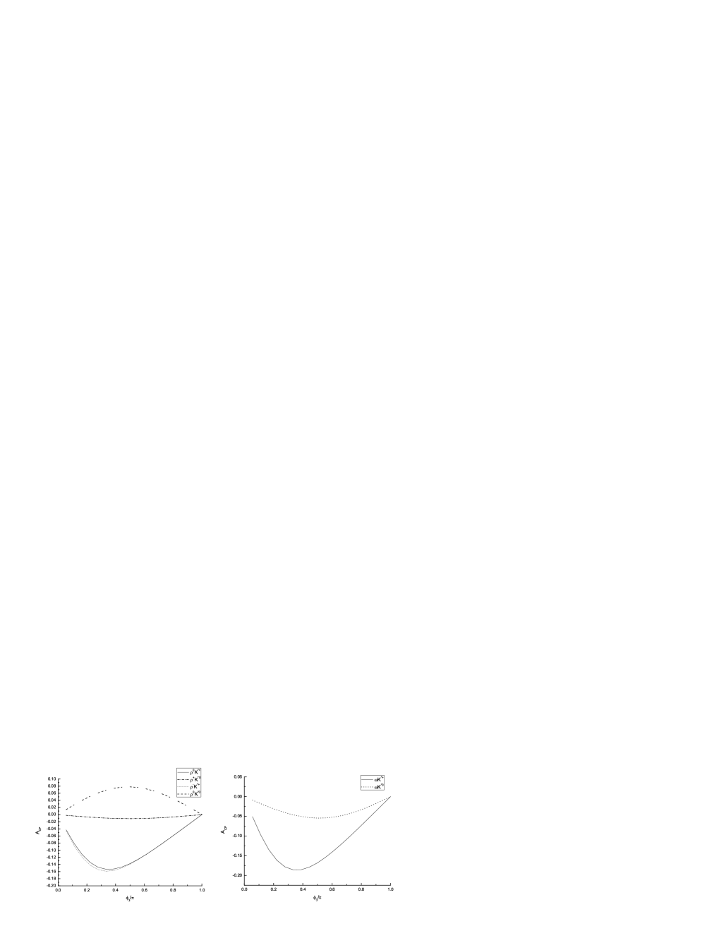
Figure 4: Direct CP violation of $B\to K^{*}\rho$ and $B\to K^{*}\omega$ as a function of CKM angle $\phi_{3}$

The angular distributions depend on the spins of the decay products of the decay vector mesons $K^{*}$ and $\rho$. For example, for $B^{+}\to K^{*+}\rho^{0}\to(K\pi)(\pi^{+}\pi^{-})$ the differential decay distribution is [41]

$$\frac{d^{3}\Gamma}{d\cos\theta_{1}d\cos\theta_{2}d\phi} = \frac{9}{8\pi}\Gamma\left\{\frac{1}{4}\frac{\Gamma_{T}}{\Gamma}\cdot\sin^{2}\theta_{1}\sin^{2}\theta_{2}+\frac{\Gamma_{L}}{\Gamma}\cdot\cos^{2}\theta_{1}\cos^{2}\theta_{2}\right.$$ (26)

$$+\frac{1}{4}\sin 2\theta_{1}\sin 2\theta_{2}[\alpha_{1}\cdot\cos\phi-\beta_{1}\cdot\sin\phi]$$

$$\left.+\frac{1}{2}\sin^{2}\theta_{1}\sin^{2}\theta_{2}\ [\alpha_{2}\cdot\cos 2\phi\ -\beta_{2}\cdot\sin 2\phi\ ]\right\}\ .$$

In (26) $\theta_{1}$ is the polar angle of the $K$ in the rest system of the $K^{*}$ with respect to the helicity axis. Similarly $\theta_{2}$ is the polar angle of the $\pi^{+}$ in the $\rho^{0}$ rest system with respect to the helicity axis of the $\rho^{0}$, and $\phi$ is the angle between the planes of the two decays $K^{*-}\to K\pi$ and $\rho^{0}\to\pi^{+}\pi^{-}$. The coefficients in the decay distribution are related to the helicity matrix elements by

$$\begin{array}[]{llllll}\frac{\Gamma_{T}}{\Gamma}&=&\frac{|M_{+1}|^{2}+|M_{-1}|^{2}}{|M_{0}|^{2}+|M_{+1}|^{2}+|M_{-1}|^{2}},&\frac{\Gamma_{L}}{\Gamma}&=&\frac{|M_{0}|^{2}}{|M_{0}|^{2}+|M_{+1}|^{2}+|M_{-1}|^{2}},\\[14.22636pt] \alpha_{1}&=&\frac{Re\left(M_{+1}M_{0}^{\ast}+M_{-1}M_{0}^{\ast}\right)}{|M_{0}|^{2}+|M_{+1}|^{2}+|M_{-1}|^{2}},&\beta_{1}&=&\frac{Im\left(M_{+1}M_{0}^{\ast}-M_{-1}M_{0}^{\ast}\right)}{|M_{0}|^{2}+|M_{+1}|^{2}+|M_{-1}|^{2}},\\[14.22636pt] \alpha_{2}&=&\frac{Re\left(M_{+1}M_{-1}^{\ast}\right)}{|M_{0}|^{2}+|M_{+1}|^{2}+|M_{-1}|^{2}},&\beta_{2}&=&\frac{Im\left(M_{+1}M_{-1}^{\ast}\right)}{|M_{0}|^{2}+|M_{+1}|^{2}+|M_{-1}|^{2}}.\\ \end{array}$$ (27)

The integration over angles $\theta_{1}$, $\theta_{2}$ in (26) yields the $\phi$ distribution of the decay width

$$2\pi\frac{d\Gamma}{d\phi} = \Gamma(1+2\alpha_{2}\cos 2\phi-2\beta_{2}\sin 2\phi),$$ (28)

where the coefficients $\alpha_{2}$, $\beta_{2}$ can be obtained from (27) by using the $M_{\lambda}$ which is calculated in PQCD approach. Because $\alpha_{2}$ and $\beta_{2}$ are very small, the decay width is almost independent in $\phi$, then the CP violation from the angular distribution will be very tiny in the standard model.

5 Summary

We performed the calculations of $B^{+}\to K^{*+}\rho^{0}$, $B^{+}\to K^{*0}\rho^{+}$, $B^{0}\to K^{*+}\rho^{-}$, $B^{0}\to K^{*0}\rho^{0}$ and $B^{+}\to K^{*+}\omega$, $B^{0}\to K^{*0}\omega$ in PQCD approach. In this approach, we calculated the non-factorizable contributions and annihilation type contributions in addition to the usual factorizable contributions.

We found that the annihilation contributions were not so small as expected in a simple argument. The annihilation diagram, which provides the dominant strong phases, plays an important role in the direct CP violations. We expect large direct CP asymmetry in the decays of $B^{+}\to K^{*+}\omega$, $B^{0}\to K^{*+}\rho^{-}$ and $B^{+}\to K^{*+}\rho^{0}$. We also study the helicity structure and angular distribution of the decay products. The current running B factories in KEK and SLAC will be able to test the theory.

Appendix A Wave Functions of Light Mesons Used in the Numerical Calculation

For the light meson wave function, we neglect the $b$ dependence part, which is not important in numerical analysis. We choose the different distribution amplitudes of ${\rho}$ meson longitudinal wave function as [34],

$$\phi_{\rho}(x) = 6f_{\rho}x(1-x)\left[1+0.18C_{2}^{3/2}(t)\right],$$ (29)

$$\phi_{\rho}^{t}(x) = f_{\rho}^{T}\left\{3t^{2}+0.3t^{2}\left[5t^{2}-3\right]+0.21\left[3-30t^{2}+35t^{4}\right]\right\},$$ (30)

$$\phi_{\rho}^{s}(x) = 3f_{\rho}^{T}~{}t\left[1+0.76(10x^{2}-10x+1)\right],$$ (31)

where $t=1-2x$. The Gegenbauer polynomials are defined by

$$\begin{array}[]{ll}C_{2}^{1/2}(t)=\frac{1}{2}(3t^{2}-1),&C_{4}^{1/2}(t)=\frac{1}{8}(35t^{4}-30t^{2}+3),\\ C_{2}^{3/2}(t)=\frac{3}{2}(5t^{2}-1),&C_{4}^{3/2}(t)=\frac{15}{8}(21t^{4}-14t^{2}+1).\end{array}$$ (32)

For the transverse $\rho$ meson we use [34]:

$$\phi_{\rho}^{T}(x) = 6f_{\rho}^{T}x(1-x)\left[1+0.2C_{2}^{3/2}(t)\right],$$ (33)

$$\phi_{\rho}^{v}(x) = f_{\rho}\left\{\frac{3}{4}(1+t^{2})+0.24(3t^{2}-1)+0.12(3-30t^{2}+35t^{4})\right\},$$ (34)

$$\phi_{\rho}^{a}(x) = \frac{3f_{\rho}}{2}~{}t\left[1+0.93(10x^{2}-10x+1)\right].$$ (35)

For the $\omega$ meson, we use the same as the above $\rho$ meson, except changing the decay constant $f_{\rho}$ with $f_{\omega}$.

We choose the light cone distribution amplitudes of ${K^{*}}$ meson longitudinal wave function as [34],

$$\phi_{K^{*}}(x) = 6f_{K^{*}}x(1-x)\left[1+0.57t+0.07C_{2}^{3/2}(t)\right],$$ (36)

$$\phi_{K^{*}}^{t}(x) = f_{K^{*}}^{T}\left\{0.3t(3t^{2}+10t-1)+1.68C_{4}^{1/2}(t)+0.06t^{2}(5t^{2}-3)\right.$$ (37)

$$\left.+0.36[1-2t-2t\ln(1-x)]\right\},$$

$$\phi_{K^{*}}^{s}(x) = f_{K^{*}}^{T}\left\{3t\left[1+0.2t+0.6(10x^{2}-10x+1)\right]-0.12x(1-x)\right.$$ (38)

$$\left.+0.36[1-6x-2\ln(1-x)]\right\}.$$

The light cone distribution amplitudes of $K^{*}$ transverse wave function are used as [34]

$$\phi_{K^{*}}^{T}(x) = 6f_{K^{*}}^{T}x(1-x)\left[1+0.6t+0.04C_{2}^{3/2}(t)\right],$$ (39)

$$\phi_{K^{*}}^{v}(x) = f_{K^{*}}\left\{\frac{3}{4}(1+t^{2}+0.44t^{3})+0.4C_{2}^{1/2}(t)+0.88C_{4}^{1/2}(t)\right.$$ (40)

$$\left.+0.48[2x+\ln(1-x)]\right\},$$

$$\phi_{K^{*}}^{a}(x) = \frac{f_{K^{*}}}{2}\left\{3t\left[1+0.19t+0.81(10x^{2}-10x+1)\right]-1.14x(1-x)\right.$$ (41)

$$\left.+0.48[1-6x-2\ln(1-x)]\right\}.$$

References

- [1] See for example: I.I. Bigi, A.I. Sanda, CP violation, Cambridge.
- [2] M. Wirbel, B. Stech, M. Bauer, Z. Phys. C29, 637 (1985); M. Bauer, B. Stech, M. Wirbel, Z. Phys. C34, 103 (1987); L.-L. Chau, H.-Y. Cheng, W.K. Sze, H. Yao, B. Tseng, Phys. Rev. D43, 2176 (1991), Erratum: D58, 019902 (1998).
- [3] A. Ali, G. Kramer and C.D. Lü, Phys. Rev. D58, 094009 (1998); C.D. Lü, Nucl. Phys. Proc. Suppl. 74, 227 (1999).
- [4] Y.-H. Chen, H.-Y. Cheng, B. Tseng, K.-C. Yang, Phys. Rev. D60, 094014 (1999); H. Y. Cheng, K. C. Yang, Phys. Rev. D 62, 054029 (2000).
- [5] M. Beneke, G. Buchalla, M. Neubert, C.T. Sachrajda, Phys. Rev. Lett. 83, 1914 (1999); M. Beneke, G. Buchalla, M. Neubert, C.T. Sachrajda, Nucl. Phys. B591, 313 (2000), M. Beneke, G. Buchalla, M. Neubert, C.T. Sachrajda, Nucl. Phys. B606, 245 (2001).
- [6] Y. Y. Keum, H.-n. Li and A. I. Sanda, Phys. Lett. B 504, 6 (2001); Phys. Rev. D63, 054008 (2001).
- [7] C.D. Lü, K. Ukai, M.Z. Yang, Phys. Rev. D63, 074009 (2001); C. D. Lu and M. Z. Yang, Eur. Phys. J. C 23, 275 (2002).
- [8] M. Beneke, Phys. Lett. B620, 143 (2005) and references cited there.
- [9] K.F. Chen, et. al, Belle Collaboration, Phys. Rev. Lett. 91, 201801 (2003).
- [10] J. Zhang, et al, Belle collaboration, Phys. Rev. Lett. 91, 221801 (2003).
- [11] B. Aubert, et at, BaBar Collaboration, Phys. Rev. Lett. 91, 171802 (2003).
- [12] A. Ali, J. G. Körner, G. Kramer and J. Willrodt, Z. Phys. C1, 269 (1979); J. G. Körner, and G. R. Goldstein, Phys. Lett. B89, 105 (1979).
- [13] Y. Grossman, Int. J. Mod. Phys. A19, 907 (2004).
- [14] Y. D. Yang, G.R. Lu, and R.M. Wang, Phys. Rev. D72, 015009 (2005).
- [15] A. L. Kagan, Phys. Lett. B601, 151 (2004); hep-ph/0407076.
- [16] C. W. Bauer, D. Pirjol, I.Z. Rothstein and I. W. Stewart, Phys. Rev. D70, 054015 (2004)
- [17] P. Colangelo, F. De. Fazio, and T. N. Pham, Phys. Lett. B597, 291 (2004); M. Ladisa, V. Laporta, G. Nardulli, P. Santorelli, Phys. Rev. D70, 114025 (2004); H. Y. Cheng, C. K. Chua, and A. D. Soni, Phys. Rev. D71, 014030 (2005).
- [18] W. S. Hou, and M. Nagashima, hep-ph/0408007.
- [19] H.-n. Li and S. Mishima, Phys. Rev. D71, 054025 (2005)
- [20] P.K. Das, K.-C. Yang, Phys. Rev. D71, 094002 (2005); K.-C. Yang, Phys. Rev. D72, 034009 (2005), Erratum-ibid. D72, 059901 (2005)
- [21] C. H. Chen, Y. Y. Keum and H.-n. Li, Phys. Rev. D66, 054013 (2002).
- [22] H.-n. Li, Phys. Lett. B622, 63 (2005).
- [23] Heavy Flavor Averaged Group, K. Anikeev et al., hep-ex/0505100, and referrences cited there.
- [24] Y.-H. Chen, H.-Y. Cheng, K.-C. Yang, Phys. Lett. B511, 40-48 (2001); X. Q. Li, G.R. Lu, and Y. D. Yang, Phys. Rev. D68, 114015 (2003).
- [25] C.H. Chang, H.N. Li, Phys. Rev. D55, 5577 (1997); T.W. Yeh and H.N. Li, Phys. Rev. D56, 1615 (1997).
- [26] G.P. Lepage and S. Brodsky, Phys. Rev. D22, 2157 (1980).
- [27] J. Botts and G. Sterman, Nucl. Phys. B225, 62 (1989).
- [28] A.G. Grozin, M. Neubert, Phys. Rev. D55, 272 (1997); M. Beneke, T. Feldmann, Nucl. Phys. B592, 3 (2001).
- [29] J. C. Collins, Acta Phys. Polon. B34, 3103 (2003)
- [30] H. S. Liao and H. N. Li, Phys. Rev. D70, 074030 (2004).
- [31] J. P. Ma and Q. Wang, Phys. Lett. B613, 39 (2005).
- [32] T. Kurimoto, H. n. Li and A. I. Sanda, Phys. Rev. D 65, 014007 (2002)
- [33] C.D. Lü and M.Z. Yang, Eur. Phys. J. C28, 515 (2003).
- [34] P. Ball, V.M. Braun, Y. Koike, and K. Tanaka, Nucl. Phys. B529, 323 (1998).
- [35] For a review, see G. Buchalla, A.J. Buras, M.E. Lautenbacher, Rev. Mod. Phys. 68, 1125 (1996).
- [36] Particle Data Group, S. Eidelman et al., Phys. Lett. B 592, 1 (2004).
- [37] M. Bauer, M. Wirbel, Z. Phys. C42, 671 (1989).
- [38] M. Bander, D. Silverman, and A. Soni, Phys. Rev. Lett. 43, 242 (1979).
- [39] V. M. Braun and A. Lenz, Phys. Rev. D 70, 074020 (2004).
- [40] B.H. Hong, C.-D. Lu, e-Print Archive: hep-ph/0505020
- [41] G. Kramer and W. F. Palmer, Phys. Rev. D 45, 193 (1992).