2005 International Linear Collider Workshop - Stanford, U.S.A.
Neutrinos in Supersymmetry

Abstract

We briefly review the neutrino mass generation mechanism in supersymmetry with Bilinear R-Parity Violation in Minimal Supergravity and Anomaly Mediated Supersymmetry Breaking.

I INTRODUCTION

Experimental results indicate that neutrinos oscillate: the three known neutrino flavour states $\nu_{e}$, $\nu_{\mu}$, and $\nu_{\tau}$, are linear combinations of the mass eigenstates $\nu_{1}$, $\nu_{2}$, and $\nu_{3}$, inducing neutrino oscillations in vacuum vacuum and in matter matter . The experimental results come from many experiments such as, Kamiokande, SAGE, GALLEX, GNO, Super-Kamiokande, and SNO for solar neutrino Fukuda:1996sz ; KamLAND for long-baseline reactor neutrino Eguchi:2002dm ; Kamiokande, Super-Kamiokande, MACRO, and Soudan-2 for atmospheric neutrino Hatakeyama:1998ea ; K2K for long-baseline accelerator neutrino Ahn:2002up ; and CHOOZ and Palo Verde for short-baseline accelerator neutrino experiments Apollonio:1999ae .

The neutrino mass matrix is diagonalized with the matrix Fogli:2005cq

$$U_{PMNS}=\left(\begin{array}[]{ccc}1&0&0\\ 0&\cos\theta_{23}&\sin\theta_{23}\\ 0&-\sin\theta_{23}&\cos\theta_{23}\end{array}\right)\left(\begin{array}[]{ccc}\cos\theta_{13}&0&\sin\theta_{13}\\ 0&1&0\\ -\sin\theta_{13}&0&\cos\theta_{13}\end{array}\right)\left(\begin{array}[]{ccc}\cos\theta_{23}&\sin\theta_{23}&0\\ -\sin\theta_{23}&\cos\theta_{23}&0\\ 0&0&1\end{array}\right)$$ (1)

This matrix may contain also a Dirac and two Majorana phases Schechter:1980gr , which we assume to be absent. The oscillations are defined by the atmospheric $\theta_{23}$, solar $\theta_{12}$ and reactor $\theta_{13}$ mixing angles, and the atmospheric $\Delta m^{2}_{32}$ and solar $\Delta m^{2}_{21}$ mass squared differences.

There are several analysis of these experimental results Nunokawa:2002mq . We use the $3\sigma$ allowed regions for the neutrino parameters in Maltoni:2004ei , given by

$$1.4\times 10^{-3}<\Delta m^{2}_{32}<3.3\times 10^{-3}\,{\mathrm{eV}}^{2} 0.52<\tan^{2}\theta_{23}<2.1$$

$$7.2\times 10^{-5}<\Delta m^{2}_{21}<9.1\times 10^{-5}\,{\mathrm{eV}}^{2} 0.30<\tan^{2}\theta_{12}<0.61$$ (2)

which we complete with the upper bound $\tan^{2}\theta_{13}<0.049$ for the reactor angle.

II LOW ENERGY SEESAW MECHANISM

We study here the generation of neutrino masses in supersymmetry with Bilinear R-Parity Violation (BRpV). The superpotential of our model differs from the MSSM by three terms which violate R-Parity and lepton number Diaz:1997xc ,

$$W=W_{MSSM}+\epsilon_{i}\hat{L}_{i}\hat{H}_{u}$$ (3)

where $\epsilon_{i}$ have units of mass. These bilinear terms induce mixing between the neutralinos and neutrinos, forming a $7\times 7$ mass matrix. A low energy seesaw mechanism induces the following effective $3\times 3$ neutrino mass matrix

$${\bf M}_{\nu}^{(0)}=\frac{M_{1}g^{2}\!+\!M_{2}{g^{\prime}}^{2}}{4\,det({\cal M}_{\chi^{0}})}\left[\matrix{\Lambda_{1}^{2}&\Lambda_{1}\Lambda_{2}&\Lambda_{1}\Lambda_{3}\cr\Lambda_{1}\Lambda_{2}&\Lambda_{2}^{2}&\Lambda_{2}\Lambda_{3}\cr\Lambda_{1}\Lambda_{3}&\Lambda_{2}\Lambda_{3}&\Lambda_{3}^{2}}\right]$$ (4)

where we have defined the parameters $\Lambda_{i}=\mu v_{i}+\epsilon_{i}v_{d}$, which are proportional to the sneutrino vacuum expectation values in the basis where the $\epsilon$ terms are removed from the superpotential. At tree-level only one neutrino acquire a mass, and one-loop corrections must be included Romao:1999up .

III ANOMALY MEDIATED SUSY BREAKING

In AMSB-BRpV we work with deCampos:2004iy ; Diaz:2002ij

$$m_{3/2}=35\,{\mathrm{TeV}}\,,\quad m_{0}=250\,{\mathrm{GeV}}\,,\quad\tan\beta=15\,,\quad\hbox{ and}\quad{\mathrm{sign}}(\mu)<0\;.$$ (5)

and we randomly vary the parameters $\epsilon_{i}$ and $\Lambda_{i}$ looking for solutions in which the restrictions (2) from neutrino physics are satisfied. An example of these solutions is

$$\epsilon_{1}=-0.015\hbox{ GeV}\;,\qquad \epsilon_{2}=-0.018\hbox{ GeV}\;,\qquad \epsilon_{3}=0.011\hbox{ GeV}\;,$$

$$\Lambda_{1}=-0.03\hbox{ GeV}^{2}\;,\qquad \Lambda_{2}=-0.09\hbox{ GeV}^{2}\;,\qquad \Lambda_{3}=-0.09\hbox{ GeV}^{2}\;.$$ (6)

The neutrino parameters obtained in this reference model are

$$\Delta m^{2}_{\mathrm{atm}}=2.4\times 10^{-3}\,{\mathrm{eV}}^{2}\,,\qquad \tan^{2}\theta_{\mathrm{atm}}=0.72\;,\qquad \tan^{2}\theta_{13}=0.033\;,$$

$$\Delta m^{2}_{\mathrm{sol}}=7.9\times 10^{-5}\,{\mathrm{eV}}^{2}\,,\qquad \tan^{2}\theta_{\mathrm{sol}}=0.47\;,\qquad$$ (7)

which agree with the present experimental results. The neutrino mass matrix has the following texture

$${\bf M}^{eff}_{\nu}=m\left[\matrix{\lambda&2\lambda&\lambda\cr 2\lambda&a&b\cr\lambda&b&1}\right]$$ (8)

with $a\sim 0.74$, $b\sim 0.67$, $\lambda\sim 0.13$, and $m\sim 0.032$ eV.

Figure 1: The red solid (blue hashed) line stands for the predicted atmospheric (solar) mass squared difference as a function of the scalar mass $m_{0}$ for $m_{3/2}=35$ TeV, $\tan\beta=15$, and $\hbox{sign}(\mu)<0$ and for the BRpV parameters given in (6). The allowed $3\sigma$ atmospheric (solar) mass squared difference is represented by the upper (lower) horizontal yellow band. Our reference point is represented by a star on the left of the plot.

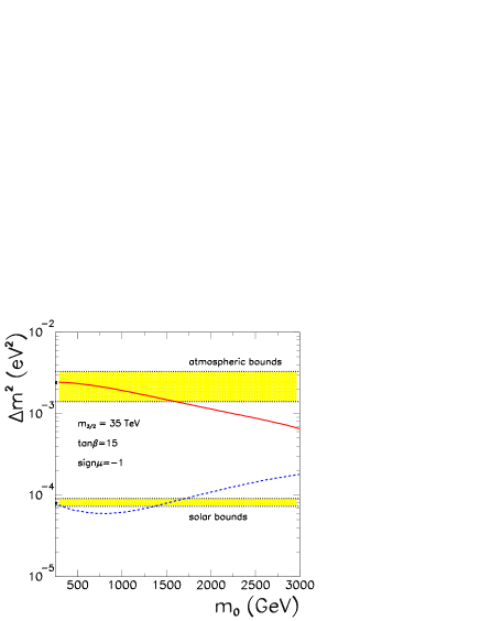
In Fig. 1 it is shown the dependence on the scalar mass $m_{0}$ of the predicted atmospheric neutrino mass squared difference $\Delta m^{2}_{\mathrm{atm}}$ (red solid line) and the solar neutrino mass squared difference $\Delta m^{2}_{\mathrm{\mathrm{sol}}}$ (blue dashed line), for fixed values $m_{3/2}=35$ TeV, $\tan\beta=15$, and $\hbox{sign}(\mu)<0$ and for the BRpV parameters given in (6). We see from Fig. 1 that $\Delta m^{2}_{\mathrm{atm}}$ is within the present experimental bounds for $m_{0}\lesssim 1.6$ TeV while $\Delta m^{2}_{\mathrm{sol}}$ satisfies the experimental constraints for $m_{0}\lesssim 310$ GeV and $1.4\hbox{ TeV}\lesssim m_{0}\lesssim 1.75$ TeV. Therefore, our models lead to acceptable neutrino masses provided $m_{0}\lesssim 310$ GeV or $1.4\hbox{ TeV}\lesssim m_{0}\lesssim 1.6$ TeV for all other parameters fixed at their reference values. It is also important to notice that the heaviest neutrino state has a mass of the order of $0.050$ eV for our reference point and that it decreases as $m_{0}$ increases. Moreover, the radiative corrections lead to a contribution of ${\cal O}(10\%)$, therefore, the tree–level result for the neutrino mass is a good order of magnitude estimative.

Figure 2: Atmospheric (solid line) and solar (dashed line) mass squared differences as a function of the gravitino mass $m_{3/2}$. The remaining parameters assume the value of our reference point and the conventions are the same of Fig. 1.

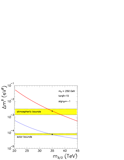
In Fig. 2 we display the dependence of the atmospheric and solar mass squared differences on the gravitino mass $m_{3/2}$ for the other parameters assuming their reference values. First of all, the observed dependence is much stronger compared to the dependence on $m_{0}$; this is expected due to the large impact of $m_{3/2}$ on the soft gaugino masses, which together with $\mu$ define the tree–level neutrino mass matrix. Moreover, the SUSY spectrum has a large impact on the one–loop corrections increasing the sensitivity to $m_{3/2}$. Both solar and atmospheric squared mass differences are too large in the region of small gravitino masses, however, this region is already partially ruled out since it leads to charginos lighter than the present experimental bounds for $m_{3/2}\lesssim 30$ TeV. Conversely, there is no acceptable solution for the neutrino masses at large $m_{3/2}$, again a region partially ruled out by data since the staus are too light in this region. Furthermore, we can see from this figure that our AMSB–BRpV model leads to acceptable neutrino masses for a small window of the gravitino mass ($33\;\rm{TeV}\lesssim m_{3/2}\lesssim 36\;\rm{TeV}$) given our choice of parameters. This is far from trivial since we have no a priori guaranty that we can generate the required neutrino spectrum, specially the radiative corrections, satisfying at the same time the experimental constraints on the superpartner masses.

IV MINIMAL SUPERGRAVITY

Our analysis in Sugra-BRpV is defined by Diaz:2004fu

$$m_{0}=100\,{\mathrm{GeV}}\,,\,M_{1/2}=250\,{\mathrm{GeV}}\,,\,A_{0}=-100\,{\mathrm{GeV}}\,,\,\tan\beta=10\,,\,\mu>0$$ (9)

where the neutralino is the LSP with a mass $m_{\chi^{0}_{1}}=99$ GeV, and the light neutral Higgs boson with $m_{h}=114$ GeV.

In this context we find several solutions for neutrino physics which satisfy the experimental constraints on the atmospheric and solar mass squared differences, and the three mixing angles. We single out the following

$$\epsilon_{1}=-0.0004\,,\qquad \epsilon_{2}=0.052\,,\qquad \epsilon_{3}=0.051\,,\,$$

$$\Lambda_{1}=0.022\,,\qquad \Lambda_{2}=0.0003\,,\qquad \Lambda_{3}=0.039\,,\,$$ (10)

This solution is characterized by

$$\Delta m^{2}_{\mathrm{atm}}=2.7\times 10^{-3}\,{\mathrm{eV}}^{2}\,,\qquad \tan^{2}\theta_{\mathrm{atm}}=0.72\;,\qquad \tan^{2}\theta_{13}=0.0058\;,$$

$$\Delta m^{2}_{\mathrm{sol}}=8.1\times 10^{-5}\,{\mathrm{eV}}^{2}\,,\qquad \tan^{2}\theta_{\mathrm{sol}}=0.54\;,\qquad$$ (11)

which are well inside the experimentally allowed window in eq. (2). We note that the random solution in eq. (10) is compatible with $\epsilon_{1}=\Lambda_{2}=0$, i.e., the neutrino parameters in eq. (11) are hardly changed with this replacement. The neutrino mass matrix has the following texture

$${\bf M}^{eff}_{\nu}=m\left[\matrix{\lambda&0&\lambda\cr 0&a&a\cr\lambda&a&1}\right]$$ (12)

with $a\sim 0.75$, $\lambda\sim 0.14$, and $m\sim 0.033$ eV.

Figure 3: Region of parameter space in the plane $m_{0}-M_{1/2}$ where solutions to neutrino physics passing all the implemented experimental cuts are located. Contours of constant atmospheric mass difference and angle, and solar mass difference are displayed.

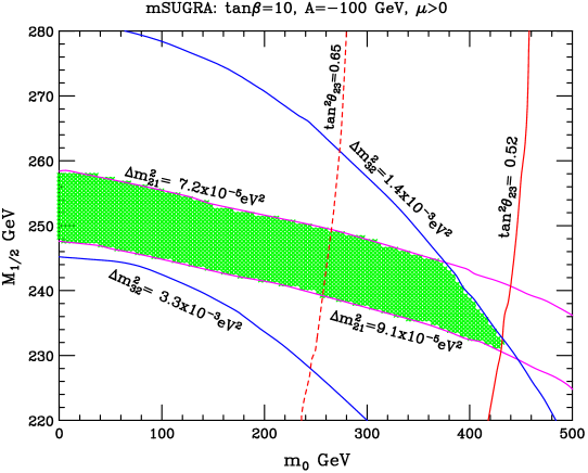
In Fig. 3 we take the neutrino solution given by the BRpV parameters in eq. (10), and vary the scalar mass $m_{0}$ and the gaugino mass $M_{1/2}$, looking for solutions that satisfy all experimental cuts. In this case, sugra points satisfying the experimental restrictions on the neutrino parameters lie in the shaded region. Solutions are concentrated in a narrow band defined by $M_{1/2}\approx 230-260$ GeV and $m_{0}\approx 0-400$ GeV. We note that in BRpV the LSP need not to be the lightest neutralino, since it is not stable anyway. For this reason, the region close to $m_{0}\approx 0$ is not ruled out.

Smaller values of $M_{1/2}$ are not possible because the atmospheric and solar mass differences become too large. The allowed strip is, thus, limited from below by the curve $\Delta m^{2}_{21}=9.1\times 10^{-5}$ eV². The dependency on $M_{1/2}$ is felt stronger by the tree level contribution. Higher values of the scalar mass $m_{0}$ are not allowed because the atmospheric angle becomes too small. The allowed strip is, therefore, limited from the right by the contour $\tan^{2}\theta_{23}=0.52$. High values of the scalar mass are also limited from above because the atmospheric mass becomes too large. Higher values of $M_{1/2}$ are not possible because the solar mass becomes too small, therefore, the allowed stripe is limited from above by the line $\Delta m^{2}_{21}=7.2\times 10^{-5}$ eV².

Figure 4: Partial decay width of a neutralino into a $W$ and a lepton, measured in units of distance.

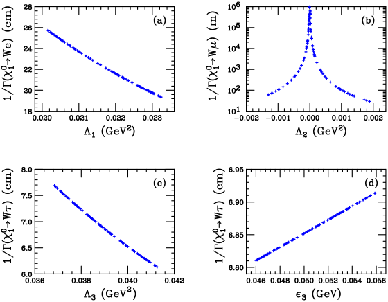
In Fig. 4 we plot the inverse of the partial decay width (multiplied by the velocity of light to convert it into a distance) as a function of the most relevant BRpV parameters. In frame (4a) we see the inverse of $\Gamma(\chi^{0}_{1}\rightarrow We)$ as a function of $\Lambda_{1}$. In fact, for all practical purposes, the decay rate into electrons depends only on $\Lambda_{1}$. Since in first approximation, the coupling is proportional to $\Lambda_{1}$, the inverse of the decay rate behaves like $\Lambda_{1}^{-2}$, and this is seen in the figure. The values of $\Lambda_{1}$ are limited by the solar parameters. The inverse of the partial decay rate $\chi^{0}_{1}\rightarrow We$ is of the order of $20-25\,cm$, and it’s an important part of the total decay rate.

In frame (4b) we have the inverse of $\Gamma(\chi^{0}_{1}\rightarrow W\mu)$ as a function of $\Lambda_{2}$, and similarly to the previous case, the decay rate into muons depends practically only on $\Lambda_{2}$. In our reference model in eq. (10) we have $\Lambda_{2}\approx 0$, but values indicated in the figure are also compatible with neutrino physics. The coupling of the neutralino to $W$ and muon is proportional to $\Lambda_{2}$, so the inverse of the decay rate goes like $\Lambda_{2}^{-2}$, and that is observed in frame (4b). Depending on the value of $\Lambda_{2}$, the partial decay length vary from centimeters to kilometers in the figure. Therefore, this partial decay rate contribute little to the total decay rate of the neutralino.

The inverse of $\Gamma(\chi^{0}_{1}\rightarrow W\tau)$ is plotted in frames (4c) and (4d) as a function of $\Lambda_{3}$ and $\epsilon_{3}$ respectively. The dependence on $\Lambda_{3}$ is stronger and similarly to the previous cases it goes like $\Lambda_{3}^{-2}$. The dependence on $\epsilon_{3}$ is weaker, and the inverse decay rate increases with this parameter. The inverse decay rate is of the order of $7\,cm$, making it the most important contribution to the total decay rate. Including the decay modes into neutrinos and a $Z$, the total inverse decay rate is near $4\,cm$. The ratios of branching ratios for our benchmark point in eq. (10) are given by

$$\frac{B(\chi^{0}_{1}\rightarrow W\mu)}{B(\chi^{0}_{1}\rightarrow W\tau)}=5.9\times 10^{-5}\,,\qquad\frac{B(\chi^{0}_{1}\rightarrow We)}{B(\chi^{0}_{1}\rightarrow W\tau)}=0.32$$ (13)

We note that if we increase $\Lambda_{2}$ by a factor 4, the first ratio of branching ratios increase to $\sim 10^{-3}$ without changing the other ratio, while still passing all the experimental cuts. From this figure, it is clear that by measuring the branching ratios of the neutralinos we get information on the parameters of the model.

We calculate the production cross sections $\sigma(pp\rightarrow\chi^{0}_{1}\chi^{0}_{1})$ (LHC) and $\sigma(e^{+}e^{-}\rightarrow\chi^{0}_{1}\chi^{0}_{1})$ (ILC at $\sqrt{s}=500$ GeV) at leading order, and using the branching ratios find

$$\sigma(pp\rightarrow\chi^{0}_{1}\chi^{0}_{1}\rightarrow W^{+}W^{+}e^{-}\tau^{-}) = 3.4\times 10^{-4}\mbox{ pb}$$

$$\sigma(e^{+}e^{-}\rightarrow\chi^{0}_{1}\chi^{0}_{1}\rightarrow W^{+}W^{+}e^{-}\tau^{-}) = 9.3\times 10^{-3}\mbox{ pb}$$ (14)

with negligible background. Assuming a luminosity of $10^{5}$ pb^-1/year at both machines, we expect $\sim 280$ signal event per year at the LHC and $\sim 3700$ signal events per year at the ILC (summing over lepton charges).

V CONCLUSIONS

Supersymmetry with Bilinear R-Parity Violation remains a viable mechanism for the generation of neutrino masses and mixing angles. In this model, the neutralino is no longer a candidate to dark matter. Nevertheless, it is possible to understand the neutrino mass spectrum. A low energy seesaw mechanism gives mass to one neutrino due to the mixing with neutralinos, and quantum corrections give mass to the other two. We show examples on how this works in supergravity and AMSB, indicating how this model can be tested in future colliders.