2005 International Linear Collider Workshop - Stanford, U.S.A. SLAC-PUB-11295
Supersymmetry Parameter Analysis with Fittino

Abstract

We present the results of a realistic global fit of the Lagrangian parameters of the Minimal Supersymmetric Standard Model to simulated data from ILC and LHC with realistic estimates of the observable uncertainties. Higher order radiative corrections are accounted for where ever possible to date. Results are obtained for a modified SPS1a MSSM benchmark scenario but they were checked not to depend critically on this assumption. Exploiting a simulated annealing algorithm, a stable result is obtained without any a priori assumptions on the fit parameters. Most of the Lagrangian parameters can be extracted at the percent level or better if theoretical uncertainties are neglected. Neither LHC nor ILC measurements alone will be sufficient to obtain a stable result. The effects of theoretical uncertainties arising from unknown higher-order corrections and parametric uncertainties are examined qualitatively. They appear to be relevant and the result motivates further precision calculations.

I INTRODUCTION

If low-energy Supersymmetry (SUSY) susy is realized in nature, the next generation of colliders, the Large Hadron Collider (LHC) and the International Linear Collider (ILC) are likely to copiously produce SUSY particles and will allow for precise measurements of their properties. Once SUSY is established experimentally, it is the main task to explore the unknown mechanism of SUSY breaking (SSB). The most general way to do so is to reconstruct the parameters of the general Minimal Supersymmetric Standard Model (MSSM) mssm parameter space, which is significantly more ambitious than a test of specific models of SUSY breaking, like e. g. minimal supergravity (mSUGRA) msugra can be tested against the data in a relative straight-forward manner (see e. g. msugrafits ) due to their small number of parameters.

The general MSSM Lagrangian contains more than 100 new parameters which are only related to each other through the unknown SSB mechanism. Many of them (like complex phases) are already limited to some extent by measurements, e.g. by the absence of neutron and electron electric dipole moments edm . Furthermore universality of first and second generation appears to be a reasonable approximation while large Yukawa couplings in the third generation lead to significant differences. Applying these constraints, the number of free parameters is reduced to 19, including the Standard Model top quark mass as a parameter to account for parametric uncertainties. It is of high interest how well this 19-dimensional parameter space can be restricted with future measurements from LHC and ILC.

The experimental collaborations ATLAS atlas and CMS CMS at the LHC have performed detailed simulations of the possibilities to extract mass information from their future data. At a future electron positron collider for collision energies up to 1 TeV, the International Linear Collider (ILC), the kinematically accessible part of the superpartner spectrum can be studied in great detail due to favorable background conditions and the well-known initial state ref:LHCILC . The attempt of an evaluation of the MSSM Lagrangian parameters and their associated errors is only useful if the experimental errors of the future measurements are known and under control. The by far best-studied SUSY scenario to serve as a basis for such an evaluation is an mSUGRA-inspired benchmark scenario, the SPS1a scenario ref:SPS . For this scenario with a relatively light superpartner spectrum, a wealth of experimental simulations exists and has recently been compiled in the framework of the international LHC/ILC study group ref:LHCILC . In this paper, we perform a global fit of the 19 MSSM parameters to those expected measurements augmented by possible measurements of topological cross-sections (i. e. cross sections times branching fractions) that will be possible at the ILC with polarized beams. Since a detailed experimental simulation for some measurements is lacking, we estimate their uncertainties conservatively from the predicted cross-sections and transferring experimental efficiency from well-studied cases.

As theoretical basis for the global fit presented in this paper we use the loop-level calculations as implemented into the program SPheno ref:SPheno . In SPheno, the masses and decay branching fractions of the superpartners are calculated as well as production cross sections in $\text{e}^{+}\text{e}^{-}$ collisions.

In this paper we present the result of a global fit of the MSSM Lagrangian parameters at the electro-weak scale for a slightly modified SPS1a benchmark scenario using the program Fittino ref:Fittino ; ref:FittinoProgram . Previous evaluations of the errors of those parameters msugrafits did not attempt to develop a strategy to extract those parameters from data without a priori knowledge. Within Fittino, special attention is given precisely to this task, i. e. to find the parameter set which is most consistent with the data in a $\chi^{2}$ minimization before a careful evaluation of errors and correlations is performed. A similar code sfitter exploits a different strategy for this task.

This paper is organized as follows. In Section II we shortly describe the approach used in Fittino. In Subsection II.1, the input observables are explained. The results of the fit and the error evaluation method are summarized in Subsection II.2 and conclusions are drawn in Section III.

II SPS1a’ FIT

From the numerous fitting options provided by Fittino we have chosen the following fit procedure to extract the low-energy Lagrangian parameters. First, in order to be independent of human bias, start values for the parameters are calculated using tree-level relations between parameters and a few observables ref:FittinoProgram . For fits with many parameters these values are not good enough to allow a fitting tool like MINUIT ref:Minuit to find the global minimum due to the amount of loop-level induced cross-dependencies between the individual sectors of the MSSM. Therefore, in a second step, the parameters are refined, using a simulated annealing approach ref:FittinoProgram ; SimAnn ; SimAnn2 . As a result, the parameter values are close to the global minimum so that a global fit using MINUIT can find the exact minimum in a third step. To determine the parameter uncertainties and correlations many individual fits with input values randomly smeared within their uncertainty range are carried out. The parameter uncertainties and the correlation matrix are derived from the spread of the fitted parameter values.

II.1 Input Observables from LHC and ILC

A number of anticipated LHC and ILC measurements serve as input observables to the fit. For the ILC, running at center-of-mass energies of 400 GeV, 500 GeV and 1 TeV is considered with 80 % electron and 60 % positron polarization. The predicted values of the observables are calculated using the following prescriptions:

• Masses:
  The experimental uncertainties of the mass measurements are taken from ref:LHCILC .

• Cross-sections:
  Only $\text{e}^{+}\text{e}^{-}$ cross-sections are included in the fit. However, the measurement of absolute cross-sections is impossible for many channels, in which only a fraction of the final states can be reconstructed. Therefore, absolute cross-section measurements are only used for the Higgs-strahlung production of the light Higgs boson, which is studied in detail in ref:HiggsBr .

• Cross-sections times branching fractions:
  Since no comprehensive study of the precision of cross-section times branching fraction measurements is available, the uncertainty is assumed to be the error of a counting experiment with the following assumptions:

  • The selection efficiency amounts to 50 %.

  • 80 % polarization of the electron beam and 60 % polarization of the positron can be achieved.

  • 500 fb^-1 per center-of-mass energy and polarization is collected.

  • The relative precision is not allowed to be better than 1 % and the absolute accuracy is at most 0.1 fb to account for systematic uncertainties.

  All production processes and decays of SUSY particles and Higgs bosons are used which have a cross-section times branching ratio value of more than 1 fb in one of the $\text{e}^{+}\text{e}^{-}$ polarization states LL, RR, LR, RL at $\sqrt{s}=400$ and $500$ GeV and LR or RL at $\sqrt{s}=1000$ GeV.

• Branching fractions:
  The three largest branching fractions of the lightest Higgs boson are included. The uncertainties on the Higgs branching fractions are taken from ref:HiggsBr .

• Standard Model parameters:
  The present uncertainties for $m_{\text{W}}$ and $m_{\text{Z}}$ are used as conservative estimates. The experimental uncertainty for the top mass $m_{\text{t}}$ is assumed to be 50 MeV ref:HiggsBr .

Table 1: The Fittino fit result for the SPS1a’ motivated scenario. The left column shows the values predicted by SPheno version 2.2.2 for this scenario, the second column exhibits the central values of the fit with unsmeared input observables, the third column displays the parameter uncertainties for the fit with experimental uncertainties only. The last column shows the parameter uncertainties for the fit with experimental and theoretical uncertainties.

Parameter	“True” value	Fit value	Uncertainty	Uncertainty
			(exp.)	(exp.+theor.)
$\tan\beta$	$10.00$	$10.00$	$0.11$	$0.15$
$\mu$	$400.4\;\text{GeV}$	$400.4\;\text{GeV}$	$1.2\;\text{GeV}$	$1.3\;\text{GeV}$
$X_{\tau}$	$-4449.\;\text{GeV}$	$-4449.\;\text{GeV}$	$20.\;\text{GeV}$	$30.\;\text{GeV}$
$M_{\tilde{e}_{R}}$	$115.60\;\text{GeV}$	$115.60\;\text{GeV}$	$0.27\;\text{GeV}$	$0.50\;\text{GeV}$
$M_{\tilde{\tau}_{R}}$	$109.89\;\text{GeV}$	$109.89\;\text{GeV}$	$0.41\;\text{GeV}$	$0.60\;\text{GeV}$
$M_{\tilde{e}_{L}}$	$181.30\;\text{GeV}$	$181.30\;\text{GeV}$	$0.10\;\text{GeV}$	$0.12\;\text{GeV}$
$M_{\tilde{\tau}_{L}}$	$179.54\;\text{GeV}$	$179.54\;\text{GeV}$	$0.14\;\text{GeV}$	$0.19\;\text{GeV}$
$X_{\text{t}}$	$-565.7\;\text{GeV}$	$-565.7\;\text{GeV}$	$3.1\;\text{GeV}$	$15.4\;\text{GeV}$
$X_{\text{b}}$	$-4935.\;\text{GeV}$	$-4935.\;\text{GeV}$	$1284.\;\text{GeV}$	$1825.\;\text{GeV}$
$M_{\tilde{q}_{R}}$	$503.\;\text{GeV}$	$503.\;\text{GeV}$	$24.\;\text{GeV}$	$27.\;\text{GeV}$
$M_{\tilde{b}_{R}}$	$497.\;\text{GeV}$	$497.\;\text{GeV}$	$8.\;\text{GeV}$	$15.\;\text{GeV}$
$M_{\tilde{t}_{R}}$	$380.9\;\text{GeV}$	$380.9\;\text{GeV}$	$2.5\;\text{GeV}$	$3.9\;\text{GeV}$
$M_{\tilde{q}_{L}}$	$523.\;\text{GeV}$	$523.\;\text{GeV}$	$10.\;\text{GeV}$	$15.\;\text{GeV}$
$M_{\tilde{t}_{L}}$	$467.7\;\text{GeV}$	$467.7\;\text{GeV}$	$3.1\;\text{GeV}$	$5.1\;\text{GeV}$
$M_{1}$	$103.27\;\text{GeV}$	$103.27\;\text{GeV}$	$0.06\;\text{GeV}$	$0.14\;\text{GeV}$
$M_{2}$	$193.45\;\text{GeV}$	$193.45\;\text{GeV}$	$0.10\;\text{GeV}$	$0.15\;\text{GeV}$
$M_{3}$	$569.\;\text{GeV}$	$569.\;\text{GeV}$	$7.\;\text{GeV}$	$7.\;\text{GeV}$
$m_{\text{A}_{\text{run}}}$	$312.0\;\text{GeV}$	$311.9\;\text{GeV}$	$4.6\;\text{GeV}$	$6.9\;\text{GeV}$
$m_{\text{t}}$	$178.00\;\text{GeV}$	$178.00\;\text{GeV}$	$0.050\;\text{GeV}$	$0.108\;\text{GeV}$
$\chi^{2}$ for unsmeared observables: $5.3\times 10^{-5}$

In order to check the influence of theoretical uncertainties on the fit results, the fit has been performed twice, once with experimental uncertainties only and a second time with experimental and theoretical uncertainties. Theoretical uncertainties for the mass predictions are scale uncertainties taken from ref:SPA . The experimental and theoretical contributions are added in quadrature. The assumed experimental and theoretical uncertainties for the masses are given in ref:LHCILC . For the cross-section and cross-section times branching fraction measurements, the smallest allowed relative precision is raised to 2 % for the fit including theoretical uncertainties (as opposed to 1 % for the fit without theoretical uncertainties). The full list of observables used in the fit and their uncertainties can be obtained from ref:Fittino .

II.2 Fit Results

The input observables described in Section II.1 are used to determine the SUSY Lagrangian parameters in a global fit under the assumptions mentioned in Section I. In total 18 SUSY parameters remain to be fitted. In addition to those, the top mass $m_{\text{t}}$ is fitted, since it strongly influences parts of the MSSM observables. Thus 19 Lagrangian parameters are simultaneously determined in this fit.

As shown in Table 1 all parameters are perfectly reconstructed at their input values. Due to the fact that the input observables are unsmeared in this fit, the final $\chi^{2}$ is close to zero at $\chi^{2}=5.3\times 10^{-5}$.

Most parameters are reconstructed to a precision better than or around 1 %. For the U(1) gaugino mass parameter $M_{1}$, an accurary below the per mil level is achieved for the fit including experimental uncertainties only. However, its precision is worse by a factor of 2 once theoretical uncertainties are included. The uncertainties on other parameters increase by up to a factor of 5 if theoretical uncertainties are taken into account, such as $X_{\text{t}}$. In order to fully benefit from the precision data provided in particular by the ILC, work must be invested to reduce uncertainties of theoretical predications.

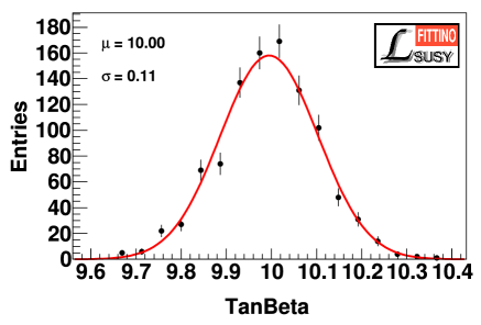
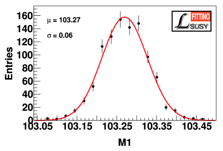
After a successful convergence of the simulated annealing algorithm to the input parameter values, the fit uncertainties are evaluated by carrying out many individual fits with input values randomly smeared within their uncertainty range using a Gaussian probability density. The complete covariance matrix and the correlation matrix are derived from the spread of the fitted parameter values. For the fit without theoretical uncertainties 1002 such fits were made. The corresponding number for the case including theory uncertainties amounts to 993. For each of those fits, the parameter set is minimized. For a large and complex parameter space with large correlations among the parameters this method has turned out to be more robust than a MINOS error analysis. An example of the outcome of this procedure for the fit (with experimental uncertainties only) is shown in Figure 1 for the parameters $\tan\beta$ and $M_{1}$ for the 1002 independent fits.

Figure 1: Examples for the parameter distributions from the toy fits. No theoretical uncertainties are included. The agreement of the parameter distributions with the Gaussian hypothesis is very good.

Figure 2: The $\chi^{2}$ distribution obtained from 1002 toy fits with smeared input distributions. The agreement with the expectation of a $\chi^{2}$ distribution with a mean of $126\pm 0.64$ is very good.

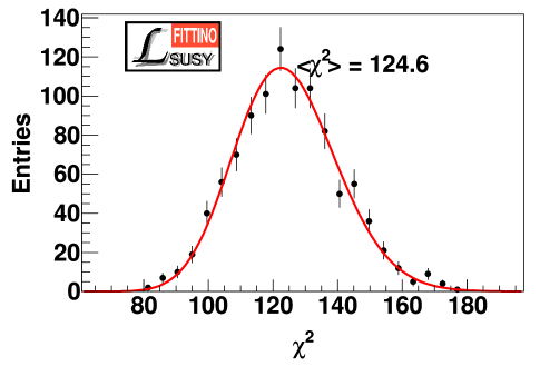
Figure 2 shows the distribution of the $\chi^{2}$ values for these 1002 independent fits for the case without theoretical uncertainties. The mean $\chi^{2}$ obtained from a fit of the $\chi^{2}$ distribution to the observed distribution is 124.6, in agreement with the expectation of 126 $\pm$ 0.64. This shows that the fits converge well to the true minimum of the $\chi^{2}$ surface for the smeared observables, implying that the uncertainties extracted from the toy fit value distributions are correct.

II.3 Relative Importance of Observables

In order to determine automatically the most important input observables influencing the precision with which a certain parameter, the contribution of each observable to $\Delta\chi^{2}=\chi^{2}_{1\sigma}-\chi^{2}_{\text{min}}$ is calculated for the parameter of interest. $\chi^{2}_{\text{min}}$ is the $\chi^{2}$ value at the minimum of the fit and $\chi^{2}_{1\sigma}$ is the corresponding value if the parameter is varied within $\pm 1\sigma$. A large $\Delta\chi^{2}$ indicates a strong correlation of the parameter with other parameters. A large contribution $\Delta\chi^{2}_{i}$ of an observable $i$ to the total $\Delta\chi^{2}$ with respect to the contributions by the other observables means that the parameter is mainly determined by the measurement of observable $i$.

Table 2: Individual $\Delta\chi^{2}$ contributions in the Fittino SPS1a’ motivated fit. In the first column the parameter and its fitted value is shown. The second column shows the total $\Delta\chi^{2}$ for this parameter, if the parameter is varied by $1\,\sigma$. The third and fourth column show the parameters and their contribution to the $\Delta\chi^{2}$ of the parameter in per cent.

Parameter	Total $\Delta\chi^{2}$	Observable	Contribution to the
Value			$\Delta\chi^{2}$ in %
$\tan\beta$	$5.0$	$\sigma(\text{e}^{-}_{L}\text{e}^{+}_{R}\rightarrow\mathrm{H}^{\pm}\mathrm{H}^{\mp}\rightarrow\mathrm{t}\bar{\mathrm{b}}\bar{\mathrm{t}}\mathrm{b})~{}1$ TeV	$31.1$
$10.00\pm 0.11$		$\sigma(\text{e}^{-}_{L}\text{e}^{+}_{R}\rightarrow\mathrm{H}\mathrm{A}\rightarrow\mathrm{b}\bar{\mathrm{b}}\mathrm{b}\bar{\mathrm{b}}~{}1)$ TeV	$9.61$
		$m_{\mathrm{h}}$	$8.12$
$\mu$	$15.2$	$\sigma(\mathrm{e}^{-}_{L}\mathrm{e}^{+}_{R}\rightarrow\tilde{\chi}^{+}_{1}\tilde{\chi}^{-}_{1}\rightarrow\bar{\nu}_{\tau}\tilde{\chi}^{0}_{1}{\tau}^{+}\,\nu_{\tau}\tilde{\chi}^{0}_{1}{\tau}^{-})~{}400$ GeV	$14.5$
$400.39\pm 1.18$ GeV		$\sigma(\mathrm{e}^{-}_{L}\mathrm{e}^{+}_{R}\rightarrow\tilde{\chi}^{+}_{1}\tilde{\chi}^{-}_{1}\rightarrow\bar{\nu}_{\tau}\tilde{\chi}^{0}_{1}{\tau}^{+}\,\nu_{\tau}\tilde{\chi}^{0}_{1}{\tau}^{-})~{}500$ GeV	$7.49$
		$\sigma(\mathrm{e}^{-}_{R}\mathrm{e}^{+}_{R}\rightarrow\tilde{\chi}^{+}_{1}\tilde{\chi}^{-}_{1}\rightarrow\bar{\nu}_{\tau}\tilde{\chi}^{0}_{1}{\tau}^{-}\,\nu_{\tau}\tilde{\chi}^{0}_{1}{\tau}^{+})~{}500$ GeV	$6.71$
$M_{\tilde{\mathrm{q}}_{R}}$	$36.6$	$m_{\tilde{\mathrm{e}}_{R}}$	$53.6$
$501.6\pm 23.6$ GeV		$m_{\tilde{\mu}_{R}}$	$3.34$
		$\sigma(\mathrm{e}^{-}_{L}\mathrm{e}^{+}_{R}\rightarrow\tilde{\chi}^{+}_{1}\tilde{\chi}^{-}_{1}\rightarrow\bar{\nu}_{\tau}\tilde{\chi}^{0}_{1}{\tau}^{-}\,\nu_{\tau}\tilde{\chi}^{0}_{1}{\tau}^{+})~{}1$ TeV	$3.25$

Generally the precision of most parameters is determined by ILC data, as shown as an example for $\tan\beta$ and $\mu$ in Table 2. As a surprise it can be seen that even for the uncertainty of the squark mass parameters the most constraining input is provided by ILC slepton mass measurements. It shows that the small contribution of the squark mass parameter $M_{\tilde{\text{q}}_{R}}$ to the slepton mass $m_{\tilde{e}_{R}}$ has a larger effect compared to the good precision of the measurement of $m_{\tilde{e}_{R}}$, than the large contribution of the squark mass parameter to the much less precisely measured squark mass.

II.4 LHC and ILC Synergy

In order to test the dependence of the fit results on the synergy of LHC and ILC, a fit has been performed with all ILC-influenced observables removed. While the LHC observables may allow to determine a further reduced set of parameters (e.g. mSUGRA, if a simplified model described by fewer parameters still fits the data), the complete set of parameters studied here is not constrained by the LHC mass observables which currently enter the fit. For most parameters, the resulting parameter uncertainties exceed the LHC+ILC uncertainties by orders of magnitude. Only for 3 of the parameters studied here, namely $M_{\tilde{\mathrm{q}}_{L}}$, $M_{\tilde{\mathrm{q}}_{R}}$ and $M_{3}$, the uncertainty is in the same order of magnitude. This exemplifies the synergy effects of the LHC and the ILC.

III CONCLUSIONS

The Lagrangian parameters of the MSSM assuming universality for the first and second generation and real parameters but without assumptions on the SUSY breaking mechanism are correctly reconstructed without usage of a priori information. This has been achieved using precision measurements at the LHC and ILC as input to a global fit exploiting the techniques implemented in the program Fittino.

Most of the Lagrangian parameters can be determined to a precision around the percent level. For some parameters an accuracy of better than 1 per mil is achievable if theoretical uncertainties are neglected. A fit including them revealed that theory uncertainties can significantly deteriorate the precision of the Lagrangian parameter determination. More work is needed to improve the accuracy of theoretical predictions in order to fully benefit from the experimental precision. The only parameter which cannot be strongly constrained by the observables used in the presented fit is $X_{\text{b}}$ resulting in a precision of only 30 % for this parameter.