MCTP-05-46

Gluino decays with heavier scalar superpartners

Manuel Toharia and James D. Wells
Michigan Center for Theoretical Physics (MCTP)
  University of Michigan, Ann Arbor, MI 48109-1120, USA

We compute gluino decay widths in supersymmetric theories with arbitrary flavor and CP violation angles. Our emphasis is on theories with scalar superpartner masses heavier than the gluino such that tree-level two-body decays are not allowed, which is relevant, for example, in split supersymmetry. We compute gluino decay branching fractions in several specific examples and show that it is plausible that the only accessible signal of supersymmetry at the LHC could be four top quarks plus missing energy. We show another example where the only accessible signal for supersymmetry is two gluon jets plus missing energy.

hep-ph/0503175

1 Introduction

A large class of supersymmetry breaking ideas predict gauginos with less mass than scalar superpartners of the standard model fermions [1]. It has been emphasized recently that a good-sized separation between the gauginos and scalars could help solve some of supersymmetry’s problems by suppressing flavor and CP violating effects, while maintaining its good features such as gauge coupling unification and dark matter.

Within these general ideas of extraordinarily heavy scalar particles [2, 3] or near PeV-scale scalars [4], there is no reason to expect the superpartner flavor angles to be diagonal, aligned or symmetrized in any way. Furthermore, there is no reason to expect the CP violating phases of soft terms to be significantly suppressed. In short, anything goes with these angles, and computation of the important phenomenological implications of these models must take into account this freedom.

Perhaps the most important phenomenological handle on split supersymmetry from a collider physics point of view is the production and decay of gluinos [4]. So far in the literature there has been no complete calculation of the gluino decay widths with arbitrary flavor angles and CP violating phases. In this article our first goal is to present a complete calculation of the gluino decays with arbitrary flavor angles and CP violating phases. Furthermore, from the structure of the amplitudes that we present, the reader can quite trivially compute gluino decays in theories where there are more neutralinos and/or charginos than the MSSM requires, as would be expected for example in a theory with an extra $U(1)$ gauge group factor.

Our second goal is to compute the gluino decay branching fractions in some interesting simplified models that can show the rich variety of possibilities that gluino decays could present to us at the LHC. For example, it is plausible that the only accessible signal of supersymmetry at the LHC could be four top quarks plus missing energy. We show another example where the only accessible signal for supersymmetry is two gluon jets plus missing energy. Many other possible phenomenologies exist, which we illustrate below.

2 Gluino decay

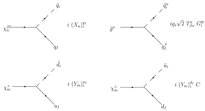
Figure 1: Generic Feynman rules for “-ino”$-$quark$-$squark interactions.

Gluino decays when the squarks are heavier than the gluino itself have been studied in the past in some models of supersymmetry. In this case gluinos can undergo a three body decay into two quarks and a neutralino or chargino [5], or decay radiatively into a gluon and a neutralino [6, 7]. With the usual universality conditions, third family squarks and sleptons can have a sizable mixing, and such effects have also been explicitly included in the literature [8].

Nevertheless, it is useful to compute the decay width formulae in a more general (and compact) way as we discussed in the introduction. We include in this section the complete formulae for gluino decays in the case where squarks are heavier than the gluino. The formulae are left in terms of the general couplings between quarks, squarks and “-inos” (gluinos, neutralinos and charginos) shown in Figure 1. Since these are generic couplings, one can add flavor mixing among squarks (unconstrained when the squarks are heavier than about $10^{5}$ GeV), CP phases, or include extra neutralinos in the spectrum. One simply has to explicitly compute the Feynman rules of Figure 1 for the desired scenario and introduce them into the formulae. After a phase space integration for the three body decays or a one-loop integration for the two body decays (both easily done numerically), one can get precise gluino decay widths for many extensions of the usual MSSM scenarios.

Definitions, conventions and notation

There are three basic types of “-ino”$-$quark$-$squark interactions which are shown in Figure 1. We define them by $(X_{n})^{q_{I}}_{i}$, $\ G^{q_{I}}_{i}$, $\ (Y_{m})^{u_{I}}_{i}$ and $(Y_{m})^{d_{I}}_{i}$.

We also need to define the “tilded” couplings in terms of the Dirac matrix $\gamma_{0}$,

$$\widetilde{G}^{q_{I}}_{i}=\gamma_{0}G^{q_{I}}_{i}\gamma_{0}\ ,\ \ \ \ \ \widetilde{X}^{q_{I}}_{i}=\gamma_{0}X_{i}^{q_{I}}\gamma_{0}\ ,\ \ \ \ \ \widetilde{Y}^{u_{I}}_{i}=\gamma_{0}Y_{i}^{u_{I}}\gamma_{0}\ \ \ {\rm and}\ \ \ \widetilde{Y}^{d_{I}}_{i}=\gamma_{0}Y_{i}^{d_{I}}\gamma_{0}\$$ (2.1)

The indices that appear in the formulae are defined as follows: the index $i$ runs through the six squarks of both up and down type $(i=1,...\,,6)$, whereas the index $I$ runs through the 3 quarks of both up and down type $(I=1,2,3)$. The index $q$ denotes the type of family in question, $up$ or $down$ $(q=u,d)$. Finally $n$ and $m$ refer to the neutralino and chargino physical states respectively. Since each chargino and neutralino are specific external particles we will generally omit their index number inside the formulae.

Decay channels and widths

We now present the complete two-body (radiative) and three-body decay widths of the gluino (in the heavy squark scenario).

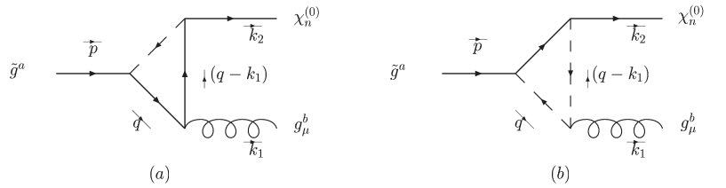
Figure 2: Diagrams contributing to the one-loop radiative gluino decay in MSSM. Due to the majorana nature of gluino and neutralino, two more diagrams contribute, but they differ only from a) and b) by having opposite fermion lines (the flow of charge inside the loop changes direction)

• $\tilde{g}\to g\chi^{o}_{\rm n}$

  The decay width for this process (see Figure 2) is

  $$\Gamma(\tilde{g}\to g\chi^{o}_{\rm n})={1\over 8\pi}{1\over 32^{2}\pi^{4}}{g^{2}}{g_{s}^{4}}\ \left({M_{\tilde{g}}^{2}-M_{\tilde{\chi}}^{2}\over M_{\tilde{g}}}\right)^{3}\ {1\over 4}{{\rm Tr}\left[{\bf\left(C_{n}\right)^{\dagger}\left(C_{n}\right)}\right]}$$ (2.2)

  where the trace is computed in Dirac Space, given the chiral structure of the coupling matrices $G^{q}_{i}$ and $X^{q}_{i}$, which are part of the effective coupling ${\bf C_{n}}$, defined by

  $${g\over\sqrt{2}}{\bf\left(C_{n}\right)}\!\! = \!\!\sum_{i,q_{I}}\left(M_{\tilde{g}}\ \left(X^{q_{I}}_{i}\widetilde{G}^{q_{I}}_{i}-\epsilon_{n}\epsilon_{g}\widetilde{X}^{{q_{I}}{{}^{\dagger}}}_{i}G^{{q_{I}}{{}^{\dagger}}}_{i}\right)\left(C_{23}+C^{\prime}_{23}+2C_{12}\right)\Big{|}_{M_{\tilde{q}_{i}},m_{q_{I}}}\right.$$ (2.3)

  $$\hskip 28.45274pt-\ M_{\tilde{\chi_{n}}}\left(\widetilde{X}^{q_{I}}_{i}{G}^{q_{I}}_{i}-\epsilon_{n}\epsilon_{g}{X}^{{q_{I}}{{}^{\dagger}}}_{i}\widetilde{G}^{{q_{I}}{{}^{\dagger}}}_{i}\right)\left(C_{23}+C^{\prime}_{23}+C_{12}\right)\Big{|}_{M_{\tilde{q}_{i}},m_{q_{I}}}$$

  $$\left.\hskip 28.45274pt\vphantom{\int}-\ m_{q_{I}}\ \left(X^{q_{I}}_{i}{G}^{q_{I}}_{i}-\epsilon_{n}\epsilon_{g}\widetilde{X}^{{q_{I}}{{}^{\dagger}}}_{i}\widetilde{G}^{{q_{I}}{{}^{\dagger}}}_{i}\right)\ C_{0}\Big{|}_{M_{\tilde{q}_{i}},m_{q_{I}}}\right).$$

  We have introduced $\epsilon_{n}$ and $\epsilon_{g}$, which denote the sign of the mass term of the $n^{th}$ neutralino and of the gluino respectively. The sum runs through all quarks and squarks.

  The functions $C_{0/12/23}\Big{|}_{M_{\tilde{q}_{i}},m_{q}}=C_{0/12/23}(0,M_{\tilde{\chi}}^{2},M_{\tilde{g}}^{2},m_{q}^{2},m_{q}^{2},M_{\tilde{q}_{i}}^{2})\$ are three-point one-loop Passarino-Veltman functions [10]. The prime denotes the interchange between $m_{q}^{2}$ and $M_{\tilde{q}_{i}}^{2}$ in the argument.
  

• $\tilde{g}\to q_{{}_{I}}\bar{q}_{{}_{J}}\chi^{o}_{\rm n}$

  

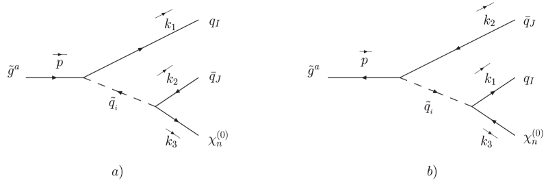
  Figure 3: Diagrams contributing to the three-body gluino decay to neutralino in MSSM.

  The decay width for this process (see Figure 3) is

  $$\Gamma(\tilde{g}\to\chi_{\rm n}^{o}q_{{}_{I}}\bar{q}_{{}_{J}})={g_{s}^{2}\over 256\pi^{3}M_{\tilde{g}}^{3}}\sum_{i,j}\int ds_{13}ds_{23}\ {1\over 2}{\cal R}e\Big{(}A_{ij}(s_{23})+B_{ij}(s_{13})-2\epsilon_{n}\epsilon_{{g}}\ C_{ij}(s_{23},s_{13})\Big{)}\ \ \ \ \ \$$ (2.4)

  where the integrand is the square of the spin-averaged total amplitude and $i,j=1,2,..,6$ are the indices of the squarks mediating the decay.

  The limits of integration are

$$s_{13}^{max}(s_{23})\!\! = \!\!m_{q_{{}_{I}}}^{2}+M_{\tilde{\chi}}^{2}+{1\over 2s_{23}}\left[(M_{\tilde{g}}^{2}-m_{q_{{}_{I}}}^{2}-s_{23})(s_{23}-m_{q_{{}_{J}}}^{2}+M_{\tilde{\chi}}^{2})+\lambda^{1/2}(s_{23},M_{\tilde{g}}^{2},m_{q_{{}_{I}}}^{2})\ \lambda^{1/2}(s_{23},m_{q_{{}_{J}}}^{2},M_{\tilde{\chi}}^{2})\right]$$

$$s_{13}^{min}(s_{23})\!\! = \!\!m_{q_{{}_{I}}}^{2}+M_{\tilde{\chi}}^{2}+{1\over 2s_{23}}\left[(M_{\tilde{g}}^{2}-m_{q_{{}_{I}}}^{2}-s_{23})(s_{23}-m_{{q_{{}_{J}}}}^{2}+M_{\tilde{\chi}}^{2})-\lambda^{1/2}(s_{23},M_{\tilde{g}}^{2},m_{q_{{}_{I}}}^{2})\ \lambda^{1/2}(s_{23},m_{q_{{}_{J}}}^{2},M_{\tilde{\chi}}^{2})\right]$$

$$s_{23}^{max}\ \ \ = (M_{\tilde{g}}-m_{q_{{}_{I}}})^{2}$$

$$s_{23}^{min}\ \ \ = (M_{\tilde{\chi}}+m_{q_{{}_{J}}})^{2}$$ (2.5)

where $\ \lambda(x,y,z)=x^{2}+y^{2}+z^{2}-2xy-2xz-2yz$ and the kinematical variables are $s_{13}=(k_{1}+k_{3})^{2}$ and $s_{23}=(k_{2}+k_{3})^{2}$.

The $A_{ij}$ terms in Eq. (2.4) represent the contributions from $diagram\ a)$ in Figure 3, whereas the $B_{ij}$ terms come from $diagram\ b)$ of the same figure.

$$A_{ij}\!\!\! = \!\!\!{\Big{(}{1\over 2}(M_{\tilde{g}}^{2}+m_{{}_{I}}^{2}-s_{23}){\rm Tr}\left[{G_{i}^{q_{{}_{I}}}G_{j}^{{q_{{}_{I}}}{{}^{\dagger}}}}\right]+m_{{}_{I}}M_{\tilde{g}}{\rm Tr}\left[{G_{i}^{q_{{}_{I}}}\widetilde{G}_{j}^{{q_{{}_{I}}}{{}^{\dagger}}}}\right]\Big{)}\Big{(}{1\over 2}(s_{23}-M_{\tilde{\chi}}^{2}-m_{{}_{J}}^{2}){\rm Tr}\left[{X^{q_{{}_{J}}}_{i}X_{j}^{q_{{}_{J}}{}^{\dagger}}}\right]-m_{{}_{J}}M_{\tilde{\chi}}{\rm Tr}\left[{X^{q_{{}_{J}}}_{i}\widetilde{X}_{j}^{q_{{}_{J}}{}^{\dagger}}}\right]\Big{)}\over\left(s_{23}-M_{\tilde{{q}}_{i}}^{2}\right)\left(s_{23}-M_{\tilde{{q}}_{j}}^{2}\right)}\ \ \ \ \ \ \ \$$

$$B_{ij}\!\!\! = \!\!\!{\Big{(}{1\over 2}(M_{\tilde{g}}^{2}+m_{{}_{J}}^{2}-s_{13}){\rm Tr}\left[{G_{i}^{q_{{}_{J}}}G_{j}^{{q_{{}_{J}}}{{}^{\dagger}}}}\right]+m_{{}_{J}}M_{\tilde{g}}{\rm Tr}\left[{G_{i}^{q_{{}_{J}}}\widetilde{G}_{j}^{{q_{{}_{J}}}{{}^{\dagger}}}}\right]\Big{)}\Big{(}{1\over 2}(s_{13}-M_{\tilde{\chi}}^{2}-m_{{}_{I}}^{2}){\rm Tr}\left[{X^{q_{{}_{I}}}_{i}X_{j}^{q_{{}_{I}}{}^{\dagger}}}\right]-m_{{}_{I}}M_{\tilde{\chi}}{\rm Tr}\left[{X^{q_{{}_{I}}}_{i}\widetilde{X}_{j}^{q_{{}_{I}}{}^{\dagger}}}\right]\Big{)}\over\left(s_{13}-M_{\tilde{{q}}_{i}}^{2}\right)\left(s_{13}-M_{\tilde{{q}}_{j}}^{2}\right)}$$

The $C_{ij}$’s represent the interference terms:

$$C_{ij} = {T_{ij}\over\left(s_{23}-M_{\tilde{{q}}_{i}}^{2}\right)\left(s_{13}-M_{\tilde{{q}}_{j}}^{2}\right)}$$ (2.6)

with $T_{ij}$ defined by

$$T_{ij}\!\!\! = \!\!\!K_{1}^{ij}\Big{[}(s_{13}\!-\!M_{\tilde{\chi}}^{2}\!-\!m_{q_{I}}^{2})(M_{\tilde{g}}^{2}\!+\!m_{q_{J}}^{2}\!-\!s_{13})\!+\!(s_{23}\!-\!M_{\tilde{\chi}}^{2}\!-\!m_{q_{J}}^{2})(M_{\tilde{g}}^{2}\!+\!m_{q_{I}}^{2}\!-\!s_{23})\!-\!(M_{\tilde{g}}^{2}\!+\!M_{\tilde{\chi}}^{2}\!-\!s_{23}\!-\!s_{13})(s_{23}\!+\!s_{13}\!-\!m_{q_{I}}^{2}-\!m_{q_{J}}^{2})\Big{]}$$

$$-\ 4M_{\tilde{\chi}}M_{\tilde{g}}m_{q_{J}}m_{q_{I}}\ K^{ij}_{2}+\ 2M_{\tilde{g}}m_{q_{J}}\left(s_{13}-M_{\tilde{\chi}}^{2}-m_{q_{I}}^{2}\right)\ K^{ij}_{3}\ +\ 2m_{q_{I}}m_{q_{J}}\left(s_{23}+s_{13}-m_{q_{I}}-m_{q_{J}}\right)\ K_{4}^{ij}\$$

$$+\ 2M_{\tilde{g}}m_{q_{I}}\left(s_{23}-M_{\tilde{\chi}}^{2}-m_{q_{J}}^{2}\right)\ K_{5}^{ij}\ -\ 2M_{\tilde{\chi}}m_{q_{J}}\left(M_{\tilde{g}}^{2}+m_{q_{I}}^{2}-s_{23}\right)\ K_{6}^{ij}\$$

$$-\ 2M_{\tilde{\chi}}M_{\tilde{g}}\left(M_{\tilde{g}}^{2}+M_{\tilde{\chi}}^{2}-s_{13}-s_{23}\right)\ K_{7}^{ij}\ -\ 2M_{\tilde{\chi}}m_{q_{I}}\left(M_{\tilde{g}}^{2}+m_{q_{J}}^{2}-s_{13}\right)\ K_{8}^{ij}\$$ (2.7)

The eight types of effective coupling constants $K_{a}^{ij}$ ($a=1,..,8$) appearing in these terms depend on the original ouplings as

$$K_{1}^{ij}={1\over 4}{\rm Tr}\left[X^{q_{{}_{J}}}_{i}\widetilde{X}_{j}^{q_{{}_{I}}{}^{\dagger}}G_{i}^{q_{{}_{I}}}\widetilde{G}_{j}^{q_{{}_{J}}{{}^{\dagger}}}\right]{\rm,}\hskip 14.22636ptK_{2}^{ij}={1\over 4}{\rm Tr}\left[X^{q_{{}_{J}}}_{i}X_{j}^{q_{{}_{I}}{}^{\dagger}}G_{i}^{q_{{}_{I}}}G_{j}^{q_{{}_{J}}{{}^{\dagger}}}\right]{\rm,}\hskip 14.22636ptK_{3}^{ij}={1\over 4}{\rm Tr}\left[X^{q_{{}_{J}}}_{i}\widetilde{X}_{j}^{q_{{}_{I}}{}^{\dagger}}{G}_{i}^{q_{{}_{I}}}{G}_{j}^{q_{{}_{J}}{{}^{\dagger}}}\right]$$

$$K_{4}^{ij}={1\over 4}{\rm Tr}\left[X^{q_{{}_{J}}}_{i}\widetilde{X}_{j}^{q_{{}_{I}}{}^{\dagger}}\widetilde{G}_{i}^{q_{{}_{I}}}G_{j}^{q_{{}_{J}}{{}^{\dagger}}}\right]{\rm,}\hskip 14.22636ptK_{5}^{ij}={1\over 4}{\rm Tr}\left[X^{q_{{}_{J}}}_{i}\widetilde{X}_{j}^{q_{{}_{I}}{}^{\dagger}}\widetilde{G}_{i}^{q_{{}_{I}}}\widetilde{G}_{j}^{q_{{}_{J}}{{}^{\dagger}}}\right]{\rm,}\hskip 14.22636ptK_{6}^{ij}={1\over 4}{\rm Tr}\left[X^{q_{{}_{J}}}_{i}X_{j}^{q_{{}_{I}}{}^{\dagger}}\widetilde{G}_{i}^{q_{{}_{I}}}G_{j}^{q_{{}_{J}}{{}^{\dagger}}}\right]$$

$$K_{7}^{ij}={1\over 4}{\rm Tr}\left[X^{q_{{}_{J}}}_{i}X_{j}^{q_{{}_{I}}{}^{\dagger}}\widetilde{G}_{i}^{q_{{}_{I}}}\widetilde{G}_{j}^{q_{{}_{J}}{{}^{\dagger}}}\right]\hskip 14.22636pt{\rm and}\hskip 14.22636ptK_{8}^{ij}={1\over 4}{\rm Tr}\left[X^{q_{{}_{J}}}_{i}X_{j}^{q_{{}_{I}}{}^{\dagger}}G_{i}^{q_{{}_{I}}}\widetilde{G}_{j}^{q_{{}_{J}}{{}^{\dagger}}}\right]$$

where the traces are computed in Dirac Space.

• $\tilde{g}\to d_{I}\bar{u}_{J}\chi^{+}_{\rm m}$

  

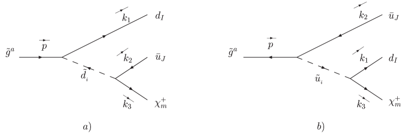
  Figure 4: Diagrams contributing to the gluino decay to chargino in the MSSM.

  The decay width of this process (see Figure 4) is

  $$\Gamma(\tilde{g}\to\chi_{\rm m}^{+}d_{{}_{I}}\bar{u}_{{}_{J}})={g_{s}^{2}\over 256\pi^{3}M_{\tilde{g}}^{3}}\sum_{i,j}\int ds_{13}ds_{23}\ {1\over 2}{\cal R}e\Big{(}A^{\prime}_{ij}(s_{23})+B^{\prime}_{ij}(s_{13})-2\epsilon_{\tilde{g}}\ C^{\prime}_{ij}(s_{23},s_{13})\Big{)}\ \ \ \ \ \ \ \$$ (2.8)

  where the integrand is the square of the spin-averaged total amplitude and $i,j=1,2,..,6$ are the indices of the squarks mediating the decay.

  The limits of integration are

$$s_{13}^{max}(s_{23})\!\!\! = \!\!\!m_{d_{{}_{I}}}^{2}\!+M_{\tilde{\chi}}^{2}+{1\over 2s_{23}}\left[(M_{\tilde{g}}^{2}-m_{d_{{}_{I}}}^{2}\!-s_{23})(s_{23}-m_{u_{{}_{J}}}^{2}\!+M_{\tilde{\chi}}^{2})+\lambda^{1/2}(s_{23},M_{\tilde{g}}^{2},m_{d_{{}_{I}}}^{2})\ \lambda^{1/2}(s_{23},m_{u_{{}_{J}}}^{2},M_{\tilde{\chi}}^{2})\right]$$

$$s_{13}^{min}(s_{23})\!\!\! = \!\!\!m_{d_{{}_{I}}}^{2}\!+M_{\tilde{\chi}}^{2}+{1\over 2s_{23}}\left[(M_{\tilde{g}}^{2}-m_{d_{{}_{I}}}^{2}\!-s_{23})(s_{23}-m_{u_{{}_{J}}}^{2}\!+M_{\tilde{\chi}}^{2})-\lambda^{1/2}(s_{23},M_{\tilde{g}}^{2},m_{d_{{}_{I}}}^{2})\ \lambda^{1/2}(s_{23},m_{u_{{}_{J}}}^{2},M_{\tilde{\chi}}^{2})\right]$$

$$s_{23}^{max}\ \ \ = (M_{\tilde{g}}-m_{d_{{}_{I}}})^{2}$$

$$s_{23}^{min}\ \ \ = (M_{\tilde{\chi}}+m_{u_{{}_{J}}})^{2},$$ (2.9)

where $\ \lambda(x,y,z)=x^{2}+y^{2}+z^{2}-2xy-2xz-2yz$ and the kinematical variables are $s_{13}=(k_{1}+k_{3})^{2}$ and $s_{23}=(k_{2}+k_{3})^{2}$.

The terms ${A}^{\prime}_{ij}$, ${B}^{\prime}_{ij}$ and ${C}^{\prime}_{ij}$ in Eq. (2.8) are

$${A}^{\prime}_{ij}\!\!\!\! = \!\!\!\!{\Big{(}{1\over 2}(M_{\tilde{g}}^{2}+m_{d_{{}_{I}}}^{2}\!-s_{23}){\rm Tr}\left[{G_{i}^{d_{{}_{I}}}G_{j}^{{d_{{}_{I}}}{{}^{\dagger}}}}\right]\!\!+m_{d_{{}_{I}}}\!M_{\tilde{g}}{\rm Tr}\left[{G^{d_{{}_{I}}}_{i}\widetilde{G}_{j}^{{d_{{}_{I}}}{{}^{\dagger}}}}\right]\Big{)}\Big{(}{1\over 2}(s_{23}-M_{\tilde{\chi}}^{2}-m_{u_{{}_{J}}}^{2}){\rm Tr}\left[{Y^{u_{{}_{J}}}_{i}Y_{j}^{{u_{{}_{J}}}{{}^{\dagger}}}}\right]\!\!-m_{u_{{}_{J}}}\!M_{\tilde{\chi}}{\rm Tr}\left[{Y^{u_{{}_{J}}}_{i}\widetilde{Y}_{j}^{{u_{{}_{J}}}{{}^{\dagger}}}}\right]\Big{)}\over\left(s_{23}-M_{\tilde{d}_{i}}^{2}\right)\left(s_{23}-M_{\tilde{d}_{j}}^{2}\right)}$$

$${B}^{\prime}_{ij}\!\!\!\! = \!\!\!\!{\Big{(}{1\over 2}(M_{\tilde{g}}^{2}+m_{u_{{}_{J}}}^{2}\!-s_{13}){\rm Tr}\left[{G^{u_{{}_{J}}}_{i}G_{j}^{{u_{{}_{J}}}{{}^{\dagger}}}}\right]+\!\!m_{u_{{}_{J}}}\!M_{\tilde{g}}{\rm Tr}\left[{G^{u_{{}_{J}}}_{i}\widetilde{G}_{j}^{{u_{{}_{J}}}{{}^{\dagger}}}}\right]\Big{)}\Big{(}{1\over 2}(s_{13}-M_{\tilde{\chi}}^{2}-m_{d_{{}_{I}}}^{2}){\rm Tr}\left[{Y_{i}^{d_{{}_{I}}}Y_{j}^{{d_{{}_{I}}}{{}^{\dagger}}}}\right]-\!\!m_{d_{{}_{I}}}\!M_{\tilde{\chi}}{\rm Tr}\left[{Y_{i}^{d_{{}_{I}}}\widetilde{Y}_{j}^{{d_{{}_{I}}}{{}^{\dagger}}}}\right]\Big{)}\over\left(s_{13}-M_{\tilde{t}_{i}}^{2}\right)\left(s_{13}-M_{\tilde{t}_{j}}^{2}\right)}$$

and

$$C^{\prime}_{ij} = {T^{\prime}_{ij}\over\left(s_{23}-M_{\tilde{b}_{i}}^{2}\right)\left(s_{13}-M_{\tilde{t}_{j}}^{2}\right)}$$ (2.10)

with

$$T^{\prime}_{ij}\!\!\!\! = \!\!\!\!{K^{\prime}_{1}}^{ij}\Big{[}(s_{13}\!-\!M_{\tilde{\chi}}^{2}\!-\!m_{d_{{}_{I}}}^{2})(M_{\tilde{g}}^{2}\!+\!m_{u_{{}_{J}}}^{2}\!\!-\!s_{13})\!+\!(s_{23}\!-\!M_{\tilde{\chi}}^{2}\!-\!m_{u_{{}_{J}}}^{2})(M_{\tilde{g}}^{2}\!+\!m_{d_{{}_{I}}}^{2}\!\!-\!s_{23})\!-\!(M_{\tilde{g}}^{2}\!+\!M_{\tilde{\chi}}^{2}\!-\!s_{23}\!-\!s_{13})(s_{23}\!+\!s_{13}\!-\!m_{d_{{}_{I}}}^{2}\!\!-\!m_{u_{{}_{J}}}^{2})\Big{]}\$$

$$-\ 4M_{\tilde{\chi}}M_{\tilde{g}}m_{d_{{}_{I}}}m_{u_{{}_{J}}}\ {K^{\prime}_{2}}^{ij}\!+\ 2M_{\tilde{g}}m_{u_{{}_{J}}}\left(s_{13}-M_{\tilde{\chi}}^{2}-m_{d_{{}_{I}}}^{2}\right)\ {K^{\prime}_{3}}^{ij}+\ 2m_{d_{{}_{I}}}m_{u_{{}_{J}}}\left(s_{23}+s_{13}-m_{d_{{}_{I}}}^{2}-m_{u_{{}_{J}}}^{2}\right)\ {K^{\prime}_{4}}^{ij}$$

$$+\ 2M_{\tilde{g}}m_{d_{{}_{I}}}\left(s_{23}-M_{\tilde{\chi}}^{2}-m_{u_{{}_{J}}}^{2}\right)\ {K^{\prime}_{5}}^{ij}-\ 2M_{\tilde{\chi}}m_{u_{{}_{J}}}\left(M_{\tilde{g}}^{2}+m_{d_{{}_{I}}}^{2}-s_{23}\right)\ {K^{\prime}_{6}}^{ij}$$

$$-\ 2M_{\tilde{\chi}}M_{\tilde{g}}\left(M_{\tilde{g}}^{2}+M_{\tilde{\chi}}^{2}-s_{13}-s_{23}\right)\ {K^{\prime}_{7}}^{ij}-\ 2M_{\tilde{\chi}}m_{d_{{}_{I}}}\left(M_{\tilde{g}}^{2}+m_{u_{{}_{J}}}^{2}-s_{13}\right)\ {K^{\prime}_{8}}^{ij}$$ (2.11)

The effective couplings ${K^{\prime}_{a}}^{ij}$ are

$${K^{\prime}_{1}}^{ij}={1\over 4}{\rm Tr}\left[Y_{i}^{u_{{}_{J}}}Y_{j}^{{d_{{}_{I}}}}G_{i}^{d_{{}_{I}}}\widetilde{G}_{j}^{{u_{{}_{J}}}{{}^{\dagger}}}\right]{\rm,}\hskip 14.22636pt{K^{\prime}_{2}}^{ij}={1\over 4}{\rm Tr}\left[Y_{i}^{u_{{}_{J}}}\widetilde{Y}_{j}^{{d_{{}_{I}}}}G_{i}^{d_{{}_{I}}}G_{j}^{{u_{{}_{J}}}{{}^{\dagger}}}\right]{\rm,}\hskip 14.22636pt{K^{\prime}_{3}}^{ij}={1\over 4}{\rm Tr}\left[Y_{i}^{u_{{}_{J}}}Y_{j}^{{d_{{}_{I}}}}{G}_{i}^{d_{{}_{I}}}{G}_{j}^{{u_{{}_{J}}}{{}^{\dagger}}}\right]$$

$${K^{\prime}_{4}}^{ij}={1\over 4}{\rm Tr}\left[Y_{i}^{u_{{}_{J}}}Y_{j}^{{d_{{}_{I}}}}\widetilde{G}_{i}^{d_{{}_{I}}}G_{j}^{{u_{{}_{J}}}{{}^{\dagger}}}\right]{\rm,}\hskip 14.22636pt{K^{\prime}_{5}}^{ij}={1\over 4}{\rm Tr}\left[Y_{i}^{u_{{}_{J}}}Y_{j}^{{d_{{}_{I}}}}\widetilde{G}_{i}^{d_{{}_{I}}}\widetilde{G}_{j}^{{u_{{}_{J}}}{{}^{\dagger}}}\right]{\rm,}\hskip 14.22636pt{K^{\prime}_{6}}^{ij}={1\over 4}{\rm Tr}\left[Y_{i}^{u_{{}_{J}}}\widetilde{Y}_{j}^{{d_{{}_{I}}}}\widetilde{G}_{i}^{d_{{}_{I}}}G_{j}^{{u_{{}_{J}}}{{}^{\dagger}}}\right]$$

$${K^{\prime}_{7}}^{ij}={1\over 4}{\rm Tr}\left[Y_{i}^{u_{{}_{J}}}\widetilde{Y}_{j}^{{d_{{}_{I}}}}\widetilde{G}_{i}^{d_{{}_{I}}}\widetilde{G}_{j}^{{u_{{}_{J}}}{{}^{\dagger}}}\right]\hskip 14.22636pt{\rm and}\hskip 14.22636pt{K^{\prime}_{8}}^{ij}={1\over 4}{\rm Tr}\left[Y_{i}^{u_{{}_{J}}}\widetilde{Y}_{j}^{{d_{{}_{I}}}}G_{i}^{d_{{}_{I}}}\widetilde{G}_{j}^{{u_{{}_{J}}}{{}^{\dagger}}}\right]$$ (2.12)

where the traces are computed in Dirac Space.

3 Application to Split Supersymmetry

We wish now to compute the branching fractions of the gluino in some examples of split supersymmetry. Our intention here is to not delve into various model building aspects of split supersymmetry, but to give the reader an understanding for how very different the possibilities can be for gluino decay phenomenology if the scalars are much heavier than the gauginos.

Despite the fact that we are interested in general low-scale parameter descriptions of the phenomenology of split supersymmetry, it is helpful at times to give names to various orderings of the gaugino mass parameters. For example, in “minimal supergravity” (mSUGRA) and in “anomaly mediated supersymmetry breaking” (AMSB), there are particular orderings of the gaugino masses:

$${\rm mSUGRA}~{}\left\{\begin{array}[]{l}M_{1}\ =\ 0.4\ M_{1/2}\\ M_{2}\ =\ 0.8\ M_{1/2}\\ M_{3}\ =\ \ 3\ M_{1/2}\end{array}\right.\hskip 28.45274pt{\rm and}\hskip 28.45274pt{\rm AMSB}~{}\left\{\begin{array}[]{l}M_{1}\ =\ 3M_{2}\\ M_{2}\ =\ \ M_{2}\\ M_{3}\ =\ 7M_{2}\end{array}\right.$$ (3.19)

For simplicity of our illustrations, we also define a common scalar mass $m_{0}$ which corresponds to the mass of all squarks with the exception of $\tilde{t}_{R}$, $\tilde{b}_{R}$ and $\tilde{Q}^{3}_{L}$. Inspired by the usual RGE effects on scalar masses, we will take the third family squarks slightly lower than $m_{0}$ depending on the value of $\tan{\beta}$. More specifically we will take

$$\begin{array}[]{c|ccc}\tan{\beta}&m_{\tilde{Q}^{3}_{L}}&m_{\tilde{b}_{R}}&m_{\tilde{t}_{R}}\\ \hline\cr\\ 30&0.8\ m_{0}&\ 0.9\ m_{0}&\ 0.6\ m_{0}\\ 1.5&0.7\ m_{0}&\ 1\ m_{0}&\ 0.4\ m_{0}\end{array}$$ (3.24)

The trilinear parameters are ignored in the scan and nominally set to $200$ GeV when a precise value is needed. With these input parameters, all mixings and physical masses are determined and inserted in the formulae given in the first section of the present paper.

3.1 Importance of 2-body decays

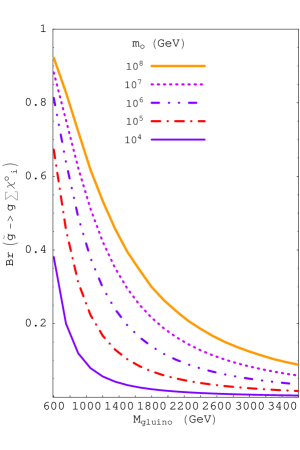
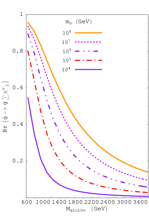
Figure 5: Radiative two-body branchings of the gluino in mSUGRA (left) and AMSB (right) with $\mu=M_{1}$ and $\tan\beta=1.5$. These two plots illustrate the argument in the text that the heavier the $gluino$ mass, the larger the scalar masses need to be for the two-body decay to be sizeable.

The ratio $R_{2/3}={\Gamma(\tilde{g}\to{\rm 2\ Body})\over\Gamma(\tilde{g}\to{\rm 3\ Body})}$ between the radiative 2-body decay width of the gluino and its total 3-body decay width into neutralinos and charginos starts to have a non-trivial scaling when the squarks mediating the decays become very heavy. When the gluino is kinematically allowed to decay into Higgsinos, $R_{2/3}$ scales with the gluino and scalar masses as

$$R_{2/3}\propto{m_{t}^{2}\left(1-\log{{M^{2}_{\tilde{t}}\over m_{t}^{2}}}\right)^{2}\over M_{\tilde{g}}^{2}}$$ (3.25)

The large $Log$ from the radiative 2-Body decay width appears out of the Passarino-Veltman function $C_{0}$ in Eq. (2.3), in the limit of large squark mass.

This $Log$ enhancement comes from the Higgsino coupling to the internal quark and squark running in the loop. It can be understood from the effective theory point of view after integrating out the heavy scalars. In that case, a four-point fermion interaction of quark-quark-gluino-higgsino can have its two quark lines tied together and a gluon can radiate from any strongly interacting particle. This diagram is divergent in the effective theory, which is cut off by the squark mass (the scale of the effective theory breakdown). The analagous construction of the two body decay from the quark-quark-gluino-wino diagram in the effective theory has no divergence, and therefore no log of the squark mass.

Thinking of these decays within the effective theory description enables us to understand that the purely diagrammatic calculation presented in this paper (and the simpler equivalent calculations in previous papers) are not entirely adequate when the scalar masses are much heavier than the gaugino masses. The large logarithm can cause a breakdown in perturbation theory for the diagrammatic calculation. To do the calculation properly in that case would require matching the effective theory with the full theory at the heavy scalar mass scale and performing a renormalization group running of operator coefficients down to the gluino scale and then computing the decay in the effective theory. We have estimated that as long as $m_{0}<10^{8}\,{\rm GeV}$ (for $M_{gluino}$ less than a few TeV) we do not have to worry about this effect, and that is one reason we are cutting off all our graphs at that scale. This does not cause us much concern in our analysis as it is our opinion that the most straightforward split supersymmetry scenarios have scalar masses only a loop level (or so) higher than the gaugino masses, which is well within the confines of our graphs.

Therefore, when the squark masses are sufficiently large, the logarithm can overcome any loop factor supression and the supression from the gluino mass squared in the denominator. Of course the heavier the gluino, the larger the scalar masses need to be for the two-body decay to be sizeable. This situation is well represented in Figure 5, where the 2-body loop-induced branching fraction of gluino decay becomes smaller as the gluino mass increases for fixed scalar mass $m_{0}$. We take the two different low scale spectra defined earlier, mSUGRA with $M_{1/2}=300$ GeV and AMSB with $M_{2}=120$ GeV. In both cases we take for this plot $\tan{\beta}=1.5$ and $\mu=M_{1}$.

Note, the $Log$ dominance occurs when the higgsino is kinematically allowed in gluino decays. If that is not the case, the lack of a $Log$ enhancement of the two-body decays means the three-body decay will generally win out. Therefore, the mass of the higgsino is of prime importance to gluino decay phenomenology.

3.2 Gluino decay phenomenology

We proceed now to describe the behavior of different branching ratios of gluino decay when the scalar mass parameter $m_{0}$ is varied between the TeV scale to $10^{8}$ GeV. In all plots a gray vertical band is located roughly between $m_{0}=10^{6}$ GeV to $m_{0}=10^{7}$ GeV. This band corresponds to the range of the total gluino decay width such that the $c\tau$ (in rest frame) is between $1mm$ and $10m$, and therefore roughly gives an estimate of where displaced vertices can be seen. To the right of the band the gluino is effectively stable (as far as the detector is concerned) and the phenomenology of that situation is studied in [9]. To the left of the band the gluino decays promptly, but the decay modes can change dramatically, depending on the scenario and the value of $m_{0}$, mostly due to the emergence of the 2-body decay channel into gluon and Higgsino.

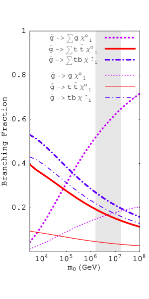
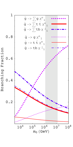
Figure 6: Branching Fractions of gluino decay for mSUGRA with $m_{1/2}=300$ GeV and $\mu=120$ GeV and with $\tan\beta=1.5$ (left) and $\tan\beta=30$ (right). The heavy scalar mass $m_{0}$ enables larger two-body final state branching fractions, as the Higgsino+gluon final state is enhanced by $\log m_{0}$ over other decay channels. The shaded band in the figure represents $1\,{\rm mm}<c\tau_{\tilde{g}}<10\,{\rm m}$.

The input parameters of Figure 6, come from mSUGRA-like low-scale relations between gaugino mass parameters, with $M_{1/2}=300$ GeV and $\mu=120$ GeV. In the left figure $\tan\beta=1.5$ which also means that we take the stop mass to be $0.4m_{0}$, slightly enhancing the stop mediated decays. In the right figure we take $\tan\beta=30$ to compare the enhancement effect. Another feature of the spectrum taken for these plots is the value of $\mu=120$ GeV such that the lightest neutralino is a mixed state of Bino and Higgsino.

In the figures we plot two types of lines, thick and thin. The thick dotted line gives the Branching fraction of gluino decay into gluon plus (any) neutralino, the thick solid line represents the decay into $t\bar{t}$ plus (any) neutralino and the thick dash-dotted line gives the $top$-$bottom$ plus (any) chargino channel.

The thin lines are really $exclusive$ and concentrate on the lightest neutralino and chargino, so that the thin dotted line represents decay into gluon plus lightest neutralino ($LSP$), the thin solid represents $t\bar{t}$ plus lightest neutralino and the thin dash-dotted line represents $bottom$-$top$ plus lightest chargino.

The two plots of Figure 6 show clearly that in the PeV scale range the 2-body decay starts to dominate over chargino and neutralino 3-body decays. Not surprisingly the decay into $t\bar{t}$ and $bt$ is enhanced for small $\tan\beta$ since the stop mediating that decay channel is clearly lighter than the rest of squarks. The $t\bar{t}$ plus neutralino Branching ranges from $0.4$ to $0.2$ in the prompt decay zone of the gluino, and can thus be an interesting signal, since between 15% and 5% of the time a pair of gluinos will give rise to at least 4 top events.

As for the exclusive signals we see that the $t\bar{t}$ plus $LSP$ branching ranges between $0.1$ and $0.05$ and monotonically decreases with $m_{0}$ due to the fact that the 2-body branching is increasing. The other interesting signal is the 2-body decay into gluon and $LSP$, the branching of which increases to values of around $0.13-0.17$ for the larger scalar masses. This mode has some importance in this case because the lightest neutralino carries some Higgsino component and therefore its radiative gluino decay increases thanks to the $Log$ enhacement discussed in the previous section. A pair of gluinos decaying into two jets plus substantial $E/$ (from two $LSP$’s) would be an interesting and unexpected result from supersymmetry.

In Fig. 7 we show the generic case for gluino decays when the gauginos follow an AMSB mass ordering. Again, there are many final states to untangle at the accelerator to determine exactly how the gluino is decaying. Also, we point out that the two body decay is decreased in the right panel of this diagram compared to the left panel due to the higgsino mass being nearly as heavy as the gluino mass. For higgsino masses above the gluino mass the dotted two body decay line would drop significantly below the three body decays to charginos.

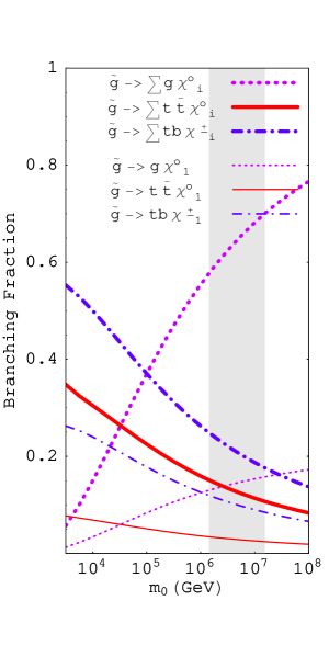
Figure 7: $M_{2}=120$, $\tan\beta=1.5$ $\mu=120$ (left), $\mu=700$ (right) AMSB. The heavy scalar mass $m_{0}$ enables larger two-body final state branching fractions, as the Higgsino+gluon final state is enhanced by $\log m_{0}$ over other decay channels. The shaded band in the figure represents $1\,{\rm mm}<c\tau_{\tilde{g}}<10\,{\rm m}$. The two panels of this figure differ in $\mu$. As $\mu$ increase (right panel) the ability to decay into Higgsinos is diminished and the two-body final state branching fraction is reduced. In the right panel, lower case $q$ means that only the five lighter quarks, $u,d,c,s,b$ are included in the decay channel, while upper case $Q$ means all six Standard Model quarks are included.

Finally, we would like to point out two cases with reasonable parameters that generate unique final state phenomenology for gluino production and decay. The two cases are represented by the two panels of Fig. 8. In both of these cases we have chosen gaugino mass parameters and higgsino mass parameters judiciously, but not wantonly, to demonstrate that the branching fraction of the gluino could go into a single final state of considerable challenge for the LHC.

In the first panel of Fig. 8 we have a case where the gluino wants to decay 100% of the time to gluon plus neutralino when the top squark mass is about a factor of 5 or more below the general scalar masses. Recall this is a reasonable assumption given renormalization group flow of top squark masses which want to be driven to lighter values from large top Yukawa coupling. The loop has light top squarks contributing to them, but the three-body decays cannot take advantage of the light top squarks since top quarks are not kinematically allowed in the final state. Therefore, loop decay to gluino plus neutralino wins.(When the top squark mass is larger and comparable to other squark masses, the three body decay wins out because there is no large relative advantage of the two-body decay over three-body decays.) The LHC phenomenology in this case would be

$$\tilde{g}\tilde{g}\to gg\chi^{0}_{1}\chi^{0}_{1}~{}{\rm(two~{}jets~{}plus~{}missing~{}energy)}$$ (3.26)

Determining that this is supersymmetry would be quite a challenge for experiment.

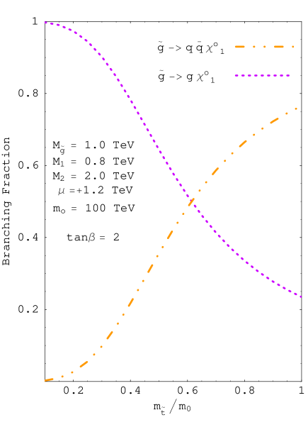
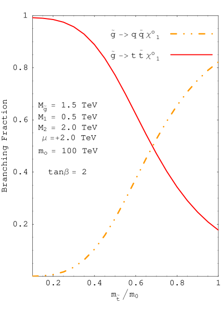
Figure 8: The two panels of this figure demonstrate the possibility of near 100% branching fraction of the gluino into a single gluon jet plus missing energy ($m_{\tilde{t}}/m_{0}<0.2$ in left panel) or near 100% branching fraction of the gluino into two top-quarks plus missing energy ($m_{\tilde{t}}/m_{0}<0.2$ in right panel). Lower case $q$ means that only the five lighter quarks $u,d,c,s,b$ are included in the decay channel

The second panel of Fig. 8 is similar to the first panel except the mass hierarchies are shuffled a bit. These rather small changes lead to a huge impact in the final state of gluino decays. In this case, the top quarks are kinematically allowed in the final state, and they win dramatically when the top squark masses are somewhat less than the other squark masses. The supersymmetry signal of this theory at the LHC is simply

$$\tilde{g}\tilde{g}\to t\bar{t}t\bar{t}\chi^{0}_{1}\chi^{0}_{1}~{}{\rm(four~{}top~{}plus~{}missing~{}energy)}$$ (3.27)

Determining that there are four top quarks in a final state would be challenging enough as it is, but to determine there is some missing energy in the event would increase the difficulty of the experiment. Given the entire spectrum of this supersymmetric model, it is possible that four tops plus missing energy could be the only signal for supersymmetry at the LHC. As there are other exotic ideas for producing four top quarks at the LHC, establishing that supersymmetry is what we are seeing would require good ideas and great experimental diligence.

Appendix: Couplings used in the numerical analysis

• Gluino couplings $G^{q_{{}_{I}}}_{i}$

  The gluino couplings are

  $$G^{q_{{}_{I}}}_{1} = \cos{\theta_{q}}\ P_{R}\ -\epsilon_{g}\ \sin{\theta_{q}}\ P_{L}$$ (A.1)

  $$G^{q_{{}_{I}}}_{2} = -\sin{\theta_{q}}\ P_{R}\ -\epsilon_{g}\ \cos{\theta_{q}}\ P_{L}$$ (A.2)

  where $P_{L/R}={1\over 2}(1\mp\gamma_{5})$.

• Neutralino couplings $X^{q_{{}_{I}}}_{i}$

  The neutralino-quark-squark interactions are

  $$X^{q_{{}_{I}}}_{1} = \cos{\theta_{q}}\ X^{q_{{}_{I}}}_{\tilde{q}_{L}}+\sin{\theta_{q}}\ X^{q_{{}_{I}}}_{\tilde{q}_{R}}$$ (A.3)

  $$X^{q_{{}_{I}}}_{2} = -\sin{\theta_{q}}\ X^{q_{{}_{I}}}_{\tilde{q}_{L}}+\cos{\theta_{q}}\ X^{q_{{}_{I}}}_{\tilde{q}_{R}}$$ (A.4)

  where we have [7]

  $$X^{t}_{\tilde{t}_{L}} = -{g\over\sqrt{2}}\left[\epsilon_{n}\Big{(}Z^{*}_{n2}+{1\over 3}\tan{\theta_{W}}\ Z^{*}_{n1}\Big{)}\ P_{L}+\ {m_{t}\over m_{W}\sin{\beta}}Z_{n4}\ P_{R}\right]$$ (A.5)

  $$X^{t}_{\tilde{t}_{R}} = -{g\over\sqrt{2}}\left[\epsilon_{n}{m_{t}\over m_{W}\sin{\beta}}Z^{*}_{n4}\ P_{L}-\Big{(}{4\over 3}\tan{\theta_{W}}\Big{)}\ Z_{n1}\ P_{R}\right]$$ (A.6)

  for the up-type quark interactions and

  $$X^{b}_{\tilde{b}_{L}} = -{g\over\sqrt{2}}\left[\epsilon_{n}\Big{(}-Z^{*}_{n2}+{1\over 3}\tan{\theta_{W}}\ Z^{*}_{n1}\Big{)}\ P_{L}\ +\ {m_{b}\over m_{W}\cos{\beta}}Z_{n3}\ P_{R}\right]$$ (A.7)

  $$X^{b}_{\tilde{b}_{R}} = -{g\over\sqrt{2}}\left[\epsilon_{n}{m_{b}\over m_{W}\cos{\beta}}Z^{*}_{n3}\ P_{L}\ +\ \Big{(}{2\over 3}\tan{\theta_{W}}\Big{)}Z_{n1}\ P_{R}\right]$$ (A.8)

  for the down-type quark.

  As usual $P_{L/R}={1\over 2}(1\mp\gamma_{5})$, and the matrix $Z$ is responsible for turning the neutral higgsinos, bino and wino into the physical neutralinos. The signs of the resulting neutralino mass terms are given by $\epsilon_{n}$ with $n=1,2,3,4$.

• Chargino couplings $Y^{t}_{i}$ and $Y^{b}_{i}$

  The Chargino-quark-squark interactions become

  $$Y^{t}_{1} = \cos{\theta_{b}}\ Y^{t}_{\tilde{b}_{L}}+\sin{\theta_{b}}\ Y^{t}_{\tilde{b}_{R}}$$ (A.9)

  $$Y^{t}_{2} = -\sin{\theta_{b}}\ Y^{t}_{\tilde{b}_{L}}+\cos{\theta_{b}}\ Y^{t}_{\tilde{b}_{R}}$$ (A.10)

  $$Y^{b}_{1} = \cos{\theta_{t}}\ Y^{b}_{\tilde{t}_{L}}+\sin{\theta_{t}}\ Y^{b}_{\tilde{t}_{R}}$$ (A.11)

  $$Y^{b}_{2} = -\sin{\theta_{t}}\ Y^{b}_{\tilde{t}_{L}}+\cos{\theta_{t}}\ Y^{b}_{\tilde{t}_{R}}$$ (A.12)

  And we have [12] for up-type quarks:

  $$Y^{t}_{\tilde{b}_{L}} = -{g\over\sqrt{2}}\ \left[\sqrt{2}\ U^{*}_{m1}\ P_{L}\ -\ {m_{t}V_{m2}\over m_{W}\sin{\beta}}\eta_{m}\ P_{R}\right]$$ (A.13)

  $$Y^{t}_{\tilde{b}_{R}} = {g\over\sqrt{2}}\ {m_{b}U^{*}_{m2}\over m_{W}\cos{\beta}}\ P_{L}$$ (A.14)

  and for down-type quarks:

  $$Y^{b}_{\tilde{t}_{L}} = {g\over\sqrt{2}}\ \left[{m_{b}U^{*}_{m2}\over m_{W}\cos{\beta}}\ P_{L}\ -\ \sqrt{2}\ V_{m1}\eta_{m}\ P_{R}\right]$$ (A.15)

  $$Y^{b}_{\tilde{t}_{R}} = {g\over\sqrt{2}}\ {m_{t}V_{m2}\over m_{W}\sin{\beta}}\eta_{m}\ P_{R}$$ (A.16)

  The matrices $U$ and $V$ are responsible for diagonalizing the Chargino mass matrix, and $\eta_{m}$ with $m=1,2$, are the signs of the resulting chargino masses.

References

[1]
For example, this is true within the AMSB approach:
L. Randall and R. Sundrum,
Nucl. Phys. B 557, 79 (1999)
[hep-th/9810155];
G. F. Giudice, M. A. Luty, H. Murayama and R. Rattazzi,
JHEP 9812, 027 (1998)
[hep-ph/9810442].
[2]
N. Arkani-Hamed and S. Dimopoulos,
hep-th/0405159;
G. F. Giudice and A. Romanino,
Nucl. Phys. B 699, 65 (2004)
[hep-ph/0406088];
N. Arkani-Hamed, S. Dimopoulos, G. F. Giudice and A. Romanino,
Nucl. Phys. B 709, 3 (2005)
[hep-ph/0409232].
[3]
A. Arvanitaki, C. Davis, P. W. Graham and J. G. Wacker,
Phys. Rev. D 70, 117703 (2004)
[hep-ph/0406034];
K. S. Babu, T. Enkhbat and B. Mukhopadhyaya,
hep-ph/0501079;
N. Haba and N. Okada,
hep-ph/0502213;
I. Antoniadis and S. Dimopoulos,
hep-th/0411032;
S. P. Martin, K. Tobe and J. D. Wells,
hep-ph/0412424;
G. Marandella, C. Schappacher and A. Strumia,
hep-ph/0502095;
B. Dutta and Y. Mimura,
hep-ph/0503052.
[4]
J. D. Wells,
hep-ph/0306127;
Phys. Rev. D 71, 015013 (2005)
[hep-ph/0411041].
[5]
R. M. Barnett, J. F. Gunion, H. E. Haber,
Phys. Rev. D37, 1892 (1988);
H. Baer, V. D. Barger, D. Karatas, X. Tata,
Phys. Rev. D36, 96 (1987);
A. Bartl, W. Majerotto, B. Mosslacher, N. Oshimo, S. Stippel,
Phys. Rev. D43, 2214 (1991).
[6]
H. E. Haber, G. L. Kane
Nucl. Phys. B232, 333 (1984);
E. Ma, G-G. Wong,
Mod. Phys. Lett. A3,1561 (1988);
R. Barbieri, G. Gamberini, G. F. Giudice, G. Ridolfi,
Nucl. Phys. B301, 15 (1988);
H. Baer, X. Tata, J. Woodside,
Phys. Rev. D42,1568 (1990).
[7]
H. E. Haber, D. Wyler,
Nucl. Phys. B323, 267 (1989).
[8] A. Bartl, W. Majerotto, W. Porod,
Z. Phys. C68, 518 (1995).
[9]
H. Baer, K. m. Cheung and J. F. Gunion,
Phys. Rev. D 59, 075002 (1999)
[hep-ph/9806361];
S. Raby and K. Tobe,
Nucl. Phys. B 539, 3 (1999)
[hep-ph/9807281];
A. Mafi and S. Raby,
Phys. Rev. D 62, 035003 (2000)
[hep-ph/9912436];
J. L. Hewett, B. Lillie, M. Masip and T. G. Rizzo,
JHEP 0409, 070 (2004)
[hep-ph/0408248];
K. Cheung and W. Y. Keung,
Phys. Rev. D 71, 015015 (2005)
[hep-ph/0408335].
[10] G. Passarino, M.J.G. Veltman,
Nucl. Phys. B160, 151 (1979).
[11] H. E. Logan.
Ph.D. Thesis (1999), hep-ph/9906332.
[12] H. E. Haber, J. F. Gunion,
Nucl. Phys. B272, 1 (1986).
[13]
P. Gambino, G. F. Giudice and P. Slavich,
[hep-ph/0506214].