We present standard model predictions for the four-fermion reaction $e^{+}e^{-}\rightarrow\mu^{+}\mu^{-}\bar{b}b$ being one of the best detection channels of a low mass Higgs boson produced through the Higgsstrahlung mechanism at a linear collider. We include leading virtual and real QED corrections due to initial state radiation and a modification of the Higgs–$b\bar{b}$ Yukawa coupling, caused by the running of the $b$-quark mass, for $e^{+}e^{-}\rightarrow\mu^{+}\mu^{-}\bar{b}b$. The complete $\mathcal{O}(\alpha)$ electroweak corrections to the $Z$–Higgs production and to the $Z$ boson decay width, as well as remaining QCD and EW corrections to the Higgs decay width, as can be calculated with a program HDECAY, are taken into account in the double pole approximation.

1 INTRODUCTION

Although the Higgs boson has not yet been discovered, its mass $m_{H}$ can be constrained in the framework of the standard model (SM) by the virtual effects it has on precision electroweak (EW) observables. Recent global fits to all precision EW data [1] give a central value of $m_{H}=114_{-40}^{+56}$ GeV and an upper limit of 241 GeV, both at 95% CL, in agreement with combined results on the direct searches for the Higgs boson at LEP that lead to a lower limit of $114.4$ GeV at 95% CL [2]. These constraints indicate the mass range where the SM Higgs boson should be searched for. If the Higgs boson exists, it is most probably to be discovered at the Large Hadron Collider, but its properties can be best investigated in a clean experimental environment of $e^{+}e^{-}$ collisions at a future International Linear Collider (ILC) [3].

Main mechanisms of the SM Higgs boson production at the ILC are the Higgsstrahlung reaction

$$e^{+}e^{-}\rightarrow ZH,$$ (1)

the $WW$ fusion

$$e^{+}e^{-}\rightarrow\nu_{e}\bar{\nu}_{e}W^{*}W^{*}\rightarrow\nu_{e}\bar{\nu}_{e}H,$$ (2)

and the $ZZ$ fusion process

$$e^{+}e^{-}\rightarrow e^{+}e^{-}Z^{*}Z^{*}\rightarrow e^{+}e^{-}H.$$ (3)

The Feynman diagrams of reactions (1), (2) and (3) are depicted in Fig. 1a,  1b and  1c, respectively.

     

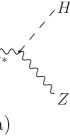
Figure 1: Feynman diagrams of reactions (1), (2) and (3), respectively.

The cross section of reaction (1) decreases according to the $1/s$ scaling law, while that of reaction (2) grows as $\ln(s/m_{H}^{2})$. Hence, while the Higgsstrahlung dominates the Higgs boson production at low energies, the $WW$ fusion process overtakes it at higher energies. The Higgs boson production rate through the $ZZ$ fusion mechanism (3) is by an order of magnitude smaller than that of process (2). The production of the SM Higgs boson in the intermediate mass range at high-energy $e^{+}e^{-}$ colliders through reaction (1) was already thoroughly studied in the literature [4]. In the present paper, we contribute further to the theoretical analysis of the Higgsstrahlung reaction by taking into account decays of the $Z$ and Higgs bosons, including the most relevant EW radiative effects both to the production and decay subprocesses. Preliminary results of the present study have been already presented in our conference paper [5].

If the Higgs boson has mass in the lower part of the range indicated above, say $m_{H}<140$ GeV, it would decay dominantly into a $\bar{b}b$ quark pair. As the $Z$ boson of reaction (1) decays into a fermion–antifermion pair too, one actually observes the Higgsstrahlung through reactions with four fermions in the final state. To be more specific, in the following we will concentrate on a four-fermion channel

$$e^{+}(p_{1})+e^{-}(p_{2})\rightarrow\mu^{+}(p_{3})+\mu^{-}(p_{4})+\bar{b}(p_{5})+b(p_{6}),$$ (4)

one of the most relevant for detection of (1) at the ILC, and the corresponding bremsstrahlung reaction

$$e^{+}(p_{1})+e^{-}(p_{2})\rightarrow\mu^{+}(p_{3})+\mu^{-}(p_{4})+\bar{b}(p_{5})+b(p_{6})+\gamma(p_{7}).$$ (5)

Both in (4) and (5), the particle four momenta have been indicated in parentheses. While final states of reactions (4) and (5) are practically not detectable in hadronic collisions because of the overwhelming QCD background, at the ILC, they should leave a particularly clear signature in a detector. To the lowest order of the SM, in the unitary gauge and neglecting the Higgs boson coupling to the electron, reactions (4) and (5) receive contributions from 34 and 236 Feynman diagrams, respectively. Typical examples of Feynman diagrams of reaction (4) are depicted in Fig. 2. The Higgsstrahlung ‘signal’ diagram is shown in Fig. 1a, while the diagrams in Figs. 1b and 1c represent typical ‘background’ diagrams. The Feynman diagrams of reaction (5) are obtained from those of reaction (4) by attaching an external photon line to each electrically charged particle line. Reactions (4) and (5) are typical examples of the neutral current four-fermion reactions and the corresponding hard bremsstrahlung reactions which had been already studied for LEP2 and TESLA TDR [3] in the case of massless fermions [6], [7] and without neglecting fermion masses [8], [9]. Reaction (4) was in particular studied in [10]. It was also considered, among other four-fermion reactions relevant for the Higgs boson production and decay, in a study of the Higgs boson searches at LEP2 performed in [11], where references to other works dedicated to the subject can be found, too.

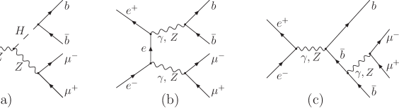
Figure 2: Examples of Feynman diagrams of reaction (4): (a) the double resonance ‘signal’, (b) and (c) ‘background’ diagrams.

In order to match the precision of data from a high luminosity linear collider, expected to be better than 1%, it is necessary to include radiative corrections in the SM predictions for reaction (4). Calculation of the complete electroweak (EW) $\mathcal{O}(\alpha)$ corrections to a four-fermion reaction like (4) is a challenging task. Problems encountered in the first attempt of such a complete calculation were described in [12]. Substantial progress in a full one-loop calculation for $e^{+}e^{-}\rightarrow u\bar{d}\mu^{-}\bar{\nu}_{\mu}$ was reported by the GRACE/1-LOOP team [13] and recently results of the first calculation of the complete EW $\mathcal{O}(\alpha)$ corrections to charged-current $e^{+}e^{-}\rightarrow 4$ fermion processes has been presented [14]. Another step towards obtaining high precision predictions for the Higgs boson production, accomplished in [15], was calculations of EW corrections to $e^{+}e^{-}\rightarrow\nu\bar{\nu}H$, a process related to (4). At the moment, however, there is no complete calculation of the corrections to neutral-current $e^{+}e^{-}\rightarrow 4$ fermion processes available that could be included into a Monte Carlo (MC) generator. Therefore it seems natural to include the leading QED corrections and to apply the double pole approximation (DPA) for the EW $\mathcal{O}(\alpha)$ corrections, as it had been done before in [16] in the case of $W$-pair production at LEP2. This means that we will include the so called factorizable EW corrections to a $ZH$ production (1) and to subprocesses of the $Z$ and Higgs decay, which are available in the literature.

To the lowest order of the SM, the cross sections of reactions (4) and (5) can be computed with a program ee4fg [17]. On the basis of ee4fg, we have written a dedicated program eezh4f that includes the following radiative corrections to (4):

• the virtual and real soft photon QED corrections to the on-shell $ZH$ production (1), a universal part of which is utilized for all Feynman diagrams of reaction (4) and combined with the initial state hard bremsstrahlung correction of (5), which we refer to as the initial state radiation (ISR) QED correction;

• the weak corrections to the $Z$–Higgs production [18], [19], i.e. the infrared (IR) finite part of the complete $\mathcal{O}(\alpha)$ EW correction to (1) and full EW corrections, including hard photon emission, to the $Z$ decay width [20], [21] in the DPA;

• the correction Higgs boson decay width, as can be computed with HDECAY [22].

The correction to the partial Higgs boson decay width $\Gamma_{H\rightarrow b\bar{b}}$ is split into two parts: one part is the tree level partial width $\Gamma^{(0)}_{H\rightarrow b\bar{b}}$ parametrized in terms of the running $b$-quark mass and the other part is the correction term that contains the remaining QCD corrections and the bulk of EW corrections, as described in [22]. The first part is included in the calculation of reactions (4) and (5) through the corresponding modification of the $H\rightarrow b\bar{b}$ Yukawa coupling, while the second part is taken into account in the DPA.

The non-factorizable corrections to (4) have not been included in eezh4f yet. Although, a comparison with the related process of $ZZ$ production and decay, where the non-factorizable corrections largely cancel each other in the total cross section [23], [24], may suggest that they are also numerically suppressed for the $ZH$-mediated four-fermion final states if decay angles are integrated over, they should be included in the program if one wants to study differential cross sections, or if one wants to improve predictions for invariant-mass distributions and similar quantities.

2 SCHEME OF THE CALCULATION

The corrections listed in the introduction are taken into account in the radiatively corrected total cross section of (4) according to the master formula

$$\int{\rm d}\sigma=\int{\rm d}\sigma_{\rm Born+r.m.}+\int_{E_{\gamma}<E_{\rm cut}}{\rm d}\sigma_{\rm virt+soft,univ.}^{\rm QED\;ISR}+\int_{E_{\gamma}>E_{\rm cut}}{\rm d}\sigma_{\rm hard}^{\rm QED\;ISR}+\int{\rm d}\sigma_{\rm virt,finite}^{\rm EW\;DPA}.$$ (6)

By ${\rm d}\sigma_{\rm Born+r.m.}$ we denote the effective Born approximation

$${\rm d}\sigma_{\rm Born+r.m.}=\frac{1}{2s}\left\{\left|M_{\rm Born}^{4f}\right|^{2}\;+2\;{\rm Re}\left(M_{\rm Born}^{4f\;^{*}}\;\delta M_{\rm r.m.}^{4f}\right)\right\}{\rm d}\Phi_{4f},$$ (7)

where $M_{\rm Born}^{4f}$ is the matrix element of reaction (4) obtained with the complete set of the lowest order Feynman diagrams, $\delta M_{\rm r.m.}^{4f}$ is the correction to the amplitude of the ‘signal’ diagram of Fig. 2(a) due to modification $\delta g_{Hb\bar{b}}^{\rm r.m.}$ of the lowest order Higgs–$b\bar{b}$ Yukawa coupling $g_{Hb\bar{b}}$ caused by the running of the $b$-quark mass, ${\rm d}\Phi_{4f}$ is the Lorentz invariant four-particle phase space element and $4f$ is a shorthand notation for the final state of reaction (4). The correction $\delta M_{\rm r.m.}^{4f}$ can be written as

$$\delta M_{\rm r.m.}^{4f} = \bar{v}\left(p_{1}\right)\left(A_{1}^{(0)}\gamma_{\mu}+A_{2}^{(0)}\gamma_{\mu}\gamma_{5}\right)u\left(p_{2}\right)\frac{-g^{\mu\nu}+p_{34}^{\mu}p_{34}^{\nu}/M_{Z}^{2}}{D_{Z}(p_{34})D_{H}(p_{56})}$$ (8)

$$\times \bar{u}\left(p_{4}\right)\left(a_{1}\gamma_{\nu}+a_{2}\gamma_{\nu}\gamma_{5}\right)v\left(p_{3}\right)\;\delta g_{Hb\bar{b}}^{\rm r.m.}\;\bar{u}(p_{6})v(p_{5}),$$

where $A_{1}^{(0)}$ and $A_{2}^{(0)}$ are the lowest order invariant amplitudes of the on-shell Higgsstrahlung reaction (1) [18] which read

$$A_{i}^{(0)}=\frac{g_{HZZ}^{(0)}}{s-M_{Z}^{2}}\;{a_{i}^{(0)}},\qquad i=1,2$$ (9)

and $D_{Z}(p_{34})$ and $D_{H}(p_{56})$ are denominators of the $Z$ and Higgs boson propagators

$$D_{Z}(p_{34})={\left(p_{3}+p_{4}\right)^{2}-M_{Z}^{2}},\qquad D_{H}(p_{56})={\left(p_{5}+p_{6}\right)^{2}-M_{H}^{2}},$$ (10)

with the complex mass parameters

$$M_{Z}^{2}=m_{Z}^{2}-im_{Z}\Gamma_{Z},\qquad M_{H}^{2}=m_{H}^{2}-im_{H}\Gamma_{H}.$$ (11)

The ‘fixed’ total widths $\Gamma_{Z}$ and $\Gamma_{H}$ of the $Z$ and Higgs bosons have been introduced in order to avoid singularities in resonant regions of the corresponding propagators. We have used the complex mass substitution also in Eq. (9), although the propagator factor of Eq. (9) can never become resonant as we want to keep open a possibility of performing calculations in the complex mass scheme [7], which preserves Ward identities.

To lowest order of the SM, the vector and axial-vector couplings of the $Z$ boson to leptons, $a_{1}^{(0)}$, $a_{2}^{(0)}$, the Higgs boson coupling to $Z$, $g_{HZZ}^{(0)}$ of Eq. (9) and the Higgs–$b\bar{b}$ Yukawa coupling, $g_{Hbb}^{(0)}$, are given by

$$a_{1}^{(0)}=\frac{4s_{W}^{2}-1}{4s_{W}c_{W}}\;e_{W},\qquad a_{2}^{(0)}=\frac{e_{W}}{4s_{W}c_{W}},\qquad g_{HZZ}^{(0)}=\frac{e_{W}m_{Z}}{s_{W}c_{W}},\qquad g_{Hbb}^{(0)}=-\frac{e_{W}m_{b}}{2s_{W}m_{W}},$$ (12)

with the effective electric charge $e_{W}=\left(4\pi\alpha_{W}\right)^{1/2}$ and electroweak mixing angle $\theta_{W}$ defined by

$$\alpha_{W}=\sqrt{2}G_{\mu}m_{W}^{2}s_{W}^{2}/\pi,\qquad{\rm and}\qquad s_{W}^{2}=1-m_{W}^{2}/m_{Z}^{2},$$ (13)

where $m_{W}$ and $m_{Z}$ are the physical masses of the $W$ and $Z$ boson, respectively. This choice, which is exactly equivalent to the $G_{\mu}$-scheme of [18], is in the program referred to as the ‘fixed width scheme’ (FWS). We have introduced usual shorthand notation $s_{W}=\sin\theta_{W}$ and $c_{W}=\cos\theta_{W}$ in Eqs. (12) and (13).

The total widths of Eq. (11) are calculated numerically in the framework of the SM: $\Gamma_{Z}$ is computed with a program based on reference [21] and $\Gamma_{H}$ is obtained with a program HDECAY [22], both programs including radiative corrections. In order not to violate unitarity it is important that we include exactly the same corrections in the amplitudes of the partial decay widths $\Gamma_{Z\rightarrow\mu^{+}\mu^{-}}$ and $\Gamma_{H\rightarrow b\bar{b}}$.

The program HDECAY includes the full massive NLO QCD corrections close to the thresholds and the massless $\mathcal{O}(\alpha^{3}_{s})$ corrections far above the thresholds. Both regions are related with a simple linear interpolation equation which, for the partial Higgs decay width $\Gamma_{H\rightarrow b\bar{b}}$ reads

$$\Gamma_{H\rightarrow b\bar{b}}=\left(1-r^{2}\right)\Gamma_{H\rightarrow b\bar{b}}\Big{(}\overline{m}_{b}(m_{H})\Big{)}+r^{2}\Gamma_{H\rightarrow b\bar{b}}\left(m_{b}\right),\qquad{\rm with}\quad r=\frac{2m_{b}}{m_{H}},$$ (14)

where large logarithms are resummed in the running $b$-quark quark mass in the $\overline{\rm MS}$ renormalization scheme $\overline{m}_{b}(m_{H})$.

By inserting the representations

$$\Gamma_{H\rightarrow b\bar{b}}\Big{(}\overline{m}_{b}(m_{H})\Big{)} = \Gamma_{H\rightarrow b\bar{b}}^{(0)}\Big{(}\overline{m}_{b}(m_{H})\Big{)}+\Delta\Gamma_{H\rightarrow b\bar{b}}\Big{(}\overline{m}_{b}(m_{H})\Big{)},$$ (15)

$$\Gamma_{H\rightarrow b\bar{b}}\left(m_{b}\right) = \Gamma_{H\rightarrow b\bar{b}}^{(0)}\left(m_{b}\right)+\Delta\Gamma_{H\rightarrow b\bar{b}}\left(m_{b}\right),$$ (16)

with the lowest order partial width into $b\bar{b}$-quark-pair given by

$$\Gamma_{H\rightarrow b\bar{b}}^{(0)}\left(m_{b}\right)=3\frac{{g_{Hb\bar{b}}^{(0)}}^{2}}{8\pi}m_{H}\left(1-\frac{4m_{b}^{2}}{m_{H}^{2}}\right)^{\frac{3}{2}},$$ (17)

into Eq. (14), we obtain the representation

$$\Gamma_{H\rightarrow b\bar{b}}=\Gamma_{H\rightarrow b\bar{b}}^{\rm r.m.}+\Delta\Gamma_{H\rightarrow b\bar{b}}$$ (18)

for $\Gamma_{H\rightarrow b\bar{b}}$. The first term on the right hand side of Eq. (18)

$$\Gamma_{H\rightarrow b\bar{b}}^{\rm r.m.}=\left(1-r^{2}\right)\Gamma_{H\rightarrow b\bar{b}}^{(0)}\Big{(}\overline{m}_{b}(m_{H})\Big{)}+r^{2}\Gamma_{H\rightarrow b\bar{b}}^{(0)}\left(m_{b}\right)$$ (19)

contains the correction due to running of the $b$-quark mass, while the second term, $\Delta\Gamma_{H\rightarrow b\bar{b}}$, incorporates the remaining QCD corrections and EW corrections that are taken into account in HDECAY.

Now, if we write the radiatively corrected Higgs–$b\bar{b}$ Yukawa coupling in the form

$$g_{Hb\bar{b}}=g_{Hb\bar{b}}^{(0)}+\delta g_{Hb\bar{b}}^{\rm r.m.}+\delta g_{Hb\bar{b}}$$ (20)

and the corrected partial Higgs decay width as

$$\Gamma_{H\rightarrow b\bar{b}} = \Gamma_{H\rightarrow b\bar{b}}^{(0)}(m_{b})\left[1+2\;{\rm Re}{\left(\frac{\delta g_{Hb\bar{b}}^{\rm r.m.}+\delta g_{Hb\bar{b}}}{g_{Hb\bar{b}}^{(0)}}\right)}\right],$$ (21)

then we will obtain the following expressions for the radiative corrections $\delta g_{Hb\bar{b}}^{\rm r.m.}$ and $\delta g_{Hb\bar{b}}$, assuming that they real,

$$\delta g_{Hb\bar{b}}^{\rm r.m.}=\frac{\Gamma_{H\rightarrow b\bar{b}}^{\rm r.m.}-\Gamma_{H\rightarrow b\bar{b}}^{(0)}(m_{b})}{2\Gamma_{H\rightarrow b\bar{b}}^{(0)}(m_{b})}\;g_{Hb\bar{b}}^{(0)},\qquad\delta g_{Hb\bar{b}}=\frac{\Gamma_{H\rightarrow b\bar{b}}-\Gamma_{H\rightarrow b\bar{b}}^{\rm r.m.}}{2\Gamma_{H\rightarrow b\bar{b}}^{(0)}(m_{b})}\;g_{Hb\bar{b}}^{(0)}.$$ (22)

We see that taking into account the correction $\delta g_{Hb\bar{b}}^{\rm r.m.}$ in Eq. (7) is actually equivalent to replacing $m_{b}$ in the lowest order Higgs–$b\bar{b}$ Yukawa coupling of Eq. (12) by some effective value of the $b$-quark mass. The same modification of the Higgs–$b\bar{b}$ Yukawa coupling is done in the soft and hard bremsstrahlung corrections represented by the second and third term on the right hand side of Eq. (6), respectively.

After having arranged the radiative corrections in the manner just described, the soft bremsstrahlung contribution of Eq. (6) can be written as

$${\rm d}\sigma_{\rm virt+soft,univ.}^{\rm QED\;ISR}={\rm d}\sigma_{\rm Born+r.m.}C_{\rm virt+soft,univ.}^{\rm QED\;ISR},$$ (23)

where the correction factor $C_{\rm virt+soft,univ.}^{\rm QED\;ISR}$,

$$C_{\rm virt+soft,univ.}^{\rm QED\;ISR}=\frac{e^{2}}{2\pi^{2}} \left[\left(\ln\frac{s}{m_{e}^{2}}-1\right)\ln\frac{2E_{\rm cut}}{\sqrt{s}}+\frac{3}{4}\ln\frac{s}{m_{e}^{2}}\right],$$ (24)

combines the universal IR singular part of the $\mathcal{O}(\alpha)$ virtual QED correction to the on-shell $ZH$ production process (1) with the soft bremsstrahlung correction to (4), integrated up to the soft photon energy cut $E_{\rm cut}$. In Eq. (23), $e$ is the electric charge that is given in terms of the fine structure constant in the Thomson limit $\alpha_{0}$, $e=\left(4\pi\alpha_{0}\right)^{1/2}$.

The third term on the right hand side of Eq. (6) represents the initial state real hard photon correction to reaction (4), i.e. the lowest order cross section of reaction (5) with the photon energy cut $E_{\gamma}>E_{\rm cut}$, which is calculated taking into account the photon emission from the initial state particles. It has been checked numerically that the dependence on $E_{\rm cut}$ cancels in the sum of the second and third term on the right hand side of Eq. (6), provided that the real photon coupling to the initial state fermions is parametrized in terms of $\alpha_{0}$, too.

Finally, the last integrand on the right hand side of Eq. (6), ${\rm d}\sigma_{\rm virt,finite}^{\rm EW,\;DPA}$, is the IR finite part of the virtual EW $\mathcal{O}(\alpha)$ correction to reaction (4) in the DPA. It can be written in the following way

$${\rm d}\sigma_{\rm virt,finite}^{\rm EW,\;DPA}=\frac{1}{2s}\left\{\left|{M^{(0)}_{DPA}}\right|^{2}{C_{\rm QED}^{\rm non-univ.}}+2{\rm Re}\left({M^{(0)^{*}}_{DPA}\delta M_{DPA}}\right)\right\}{\rm d}\Phi_{4f},$$ (25)

where the lowest order matrix element $M^{(0)}_{DPA}$ and the one-loop correction $\delta M_{DPA}$ in the DPA, which are given below, are calculated with the projected four momenta $k_{i}$, $i=3,...,6$, of the final state particles, except for denominators of the $Z$ and Higgs boson propagators. The projected four momenta are obtained from the four momenta $p_{i}$, $i=3,...,6$, of reaction (4) with a, to some extent arbitrary, projection procedure which will be defined later; $C_{\rm QED}^{\rm non-univ.}$ denotes the IR finite non universal constant part of the $\mathcal{O}(\alpha)$ QED correction that has not been taken into account in Eq. (24). It reads

$$C^{\rm QED\;ISR}_{\rm non-univ.}=\frac{e^{2}}{2\pi^{2}}\left(\frac{\pi^{2}}{6}-1\right).$$ (26)

The matrix elements $M^{(0)}_{DPA}$ and $\delta M_{DPA}$ for the $Z$ and Higgs boson production and decay of Eq. (25) are given by

$$M^{(0)}_{DPA} = -\bar{v}\left(p_{1}\right)\left(A_{1}^{(0)}\gamma_{\mu}+A_{2}^{(0)}\gamma_{\mu}\gamma_{5}\right)u\left(p_{2}\right)\frac{1}{D_{Z}(p_{34})D_{H}(p_{56})}{N}_{Z}^{\mu}\;{N}_{H},$$ (27)

$$\delta M_{DPA} = -\left\{\bar{v}\left(p_{1}\right)\bigg{[}\delta A_{1}\gamma_{\mu}+\delta A_{2}\gamma_{\mu}\gamma_{5}+\left(A_{31}p_{1\mu}+A_{32}p_{2\mu}\right)/\!\!\!k_{Z}\right.$$

$$\qquad\qquad\qquad\qquad\qquad\;\,+\left(A_{41}p_{1\mu}+A_{42}p_{2\mu}\right)/\!\!\!k_{Z}\gamma_{5}\bigg{]}u\left(p_{2}\right){N}_{Z}^{\mu}\;{N}_{H}$$

$$+\left.\bar{v}\left(p_{1}\right)\left(A_{1}^{(0)}\gamma_{\mu}+A_{2}^{(0)}\gamma_{\mu}\gamma_{5}\right)u\left(p_{2}\right)\bigg{(}\delta N_{Z}^{\mu}\;N_{H}+N_{Z}^{\mu}\;\delta N_{H}\bigg{)}\right\}\frac{1}{D_{Z}(p_{34})D_{H}(p_{56})},$$

with denominators of the $Z$ and Higgs boson propagators defined by Eq. (10) and amplitudes of decay subprocesses given by

$${N}_{Z}^{\mu}=\bar{u}\left(k_{4}\right)\left(a_{1}^{(0)}\gamma^{\mu}+a_{2}^{(0)}\gamma^{\mu}\gamma_{5}\right)v\left(k_{3}\right),\qquad{N}_{H}=g_{Hbb}^{(0)}\;\bar{u}\left(k_{6}\right)v\left(k_{5}\right)$$ (29)

in the lowest order and

$${\delta N}_{Z}^{\mu}=\bar{u}\left(k_{4}\right)\left(\delta a_{1}\gamma^{\mu}+\delta a_{2}\gamma^{\mu}\gamma_{5}\right)v\left(k_{3}\right),\qquad{\delta N}_{H}=\delta g_{Hbb}\;\bar{u}\left(k_{6}\right)v\left(k_{5}\right)$$ (30)

in the one-loop and higher order. Let us note that the invariant amplitudes $\delta a_{1}$, $\delta a_{2}$ and $\delta g_{Hbb}$ contain the QED correction factors, which include the hard photon emission. We have neglected the so-called longitudinal part of the $Z$-boson propagator proportional to $p_{34}^{\mu}p_{34}^{\nu}$ in Eqs. (27) and (2). Keeping this part would lead to some ambiguity, as the propagator couples to the final state currents $N_{Z}^{\mu}$ and $\delta N_{Z}^{\mu}$ which are parametized in terms of the projected momenta $k_{3}$ and $k_{4}$. The neglected term is of the order of $m_{\mu}$, which is consistent with neglect of the $\mathcal{O}(m_{\mu})$ terms in calculation of the one-loop EW decay amplitudes $\delta a_{1}$ and $\delta a_{2}$ of Eq. (30).

The invariant amplitudes of Eq. (2)

$$\delta A_{i}=\delta A_{i}(s,\cos\theta),\qquad A_{ji}=A_{ji}(s,\cos\theta),\quad i=1,2,\quad j=3,4,$$ (31)

represent the IR finite parts of the EW one-loop correction to the on-shell $Z$–Higgs production process (1). They are complex functions of $s=(p_{1}+p_{2})^{2}$ and $\cos\theta$, $\theta$ being the Higgs boson production angle with respect to the initial positron beam in the centre of mass system (CMS), computed with the program eezh4f. The latter makes use of the program worked out in [18] and the package FF 2.0. The package FF written by G. J. van Oldenborgh allows to evaluate one-loop integrals [25]. Note that we have changed a little the notation in Eq. (2) with respect to that of Eq. (2.5) of [18]. The IR finite contributions to the EW one-loop form factors of the $Zll$-vertex $\delta a_{1}$, $\delta a_{1}$ and the correction $\delta g_{Hbb}$ of the $Hb\bar{b}$-vertex of Eq. (30) are also calculated numerically following references [21] and [22].

As the computation of the one-loop electroweak amplitudes of Eq. (31) slows down the MC integration substantially, a simple interpolation routine has been written that samples the amplitudes at a few hundred values of $\cos\theta$ and then the amplitudes for all intermediate values of $\cos\theta$ are obtained by a linear interpolation. This gives a tremendous gain in the speed of computation, while there is practically no difference between the results obtained with the interpolation routine and without it.

We end this section with a description of the projection procedure we have applied in the program. The projected momenta $k_{Z}$ and $k_{i}$, of Eqs. (2), (29) and (30) are obtained from the four momenta $p_{i}$, $i=3,...,6$, of the final state fermions of reaction (4) with the following projection procedure.

First the on-shell momenta and energies of the Higgs and $Z$ boson in the CMS are fixed by $\displaystyle\left|\vec{k}_{H}\right|$ $\displaystyle=$ $\displaystyle\frac{\lambda^{\frac{1}{2}}\left(s,m_{Z}^{2},m_{H}^{2}\right)}{2s^{\frac{1}{2}}},$ $\displaystyle E_{H}$ $\displaystyle=$ $\displaystyle\left(\vec{k}_{H}^{2}+m_{H}^{2}\right)^{\frac{1}{2}},$ $\displaystyle\vec{k}_{H}$ $\displaystyle=$ $\displaystyle\left|\vec{k}_{H}\right|\frac{\vec{p}_{5}+\vec{p}_{6}}{\left|\vec{p}_{5}+\vec{p}_{6}\right|},$ $\displaystyle\vec{k}_{Z}$ $\displaystyle=$ $\displaystyle-\vec{k}_{H},\quad E_{Z}=\sqrt{s}-E_{H}.$

Next the four momenta $p_{5}$ and $p_{3}$ of reaction (4) are boosted to the rest frame of the $b\bar{b}$- and $\mu^{+}\mu^{-}$-pairs, respectively, where they are denoted by $p^{\prime}_{5}$ and $p^{\prime}_{3}$. The projected four momenta $k^{\prime}_{i}$, $i=5,6$, in the rest frame of the $b\bar{b}$-pair are then obtained by the kinematical relations
$\displaystyle\qquad\qquad\left|\vec{k^{\prime}}_{5}\right|$ $\displaystyle=$ $\displaystyle\frac{\lambda^{\frac{1}{2}}\left(m_{H}^{2},m_{5}^{2},m_{6}^{2}\right)}{2m_{H}},$ $\displaystyle\vec{k^{\prime}}_{6}$ $\displaystyle=$ $\displaystyle-\vec{k^{\prime}}_{5},$ $\displaystyle\vec{k^{\prime}}_{5}$ $\displaystyle=$ $\displaystyle\left|\vec{k^{\prime}}_{5}\right|\frac{\vec{p^{\prime}}_{5}}{\left|\vec{p^{\prime}}_{5}\right|},$ $\displaystyle{E^{\prime}}_{i}$ $\displaystyle=$ $\displaystyle\left(\vec{k^{\prime}}_{i}^{2}+m_{i}^{2}\right)^{\frac{1}{2}},\quad i=5,6.$ Similarly, one obtains $k^{\prime}_{3}$ and $k^{\prime}_{4}$ in the rest frame of the $\mu^{+}\mu^{-}$-pair using
$\displaystyle\qquad\qquad\left|\vec{k^{\prime}}_{3}\right|$ $\displaystyle=$ $\displaystyle\frac{\lambda^{\frac{1}{2}}\left(m_{Z}^{2},m_{3}^{2},m_{4}^{2}\right)}{2m_{Z}},$ $\displaystyle\vec{k^{\prime}}_{4}$ $\displaystyle=$ $\displaystyle-\vec{k^{\prime}}_{3},$ $\displaystyle\vec{k^{\prime}}_{3}$ $\displaystyle=$ $\displaystyle\left|\vec{k^{\prime}}_{3}\right|\frac{\vec{p^{\prime}}_{3}}{\left|\vec{p^{\prime}}_{3}\right|},$ $\displaystyle{E^{\prime}}_{i}$ $\displaystyle=$ $\displaystyle\left(\vec{k^{\prime}}_{i}^{2}+m_{i}^{2}\right)^{\frac{1}{2}},\quad i=3,4.$

The four momenta $k^{\prime}_{i}$, $i=3,...,6$, are then boosted back to the CMS giving the projected four momenta $k_{i}$, $i=3,...,6$ of $\mu^{+},\mu^{-},\bar{b}$ and $b$ that satisfy the necessary on-shell relations

$$k_{3}^{2}=k_{4}^{2}\!\!\! = \!\!\!m_{\mu}^{2},\qquad k_{5}^{2}=k_{6}^{2}=m_{b}^{2},$$

$$\left(k_{3}+k_{4}\right)^{2}\!\!\! = \!\!\!m_{Z}^{2},\qquad\left(k_{5}+k_{6}\right)^{2}=m_{H}^{2}.$$

The actual value of $\cos\theta$ in Eq. (31) is given by $\cos\theta=k_{H}^{3}/|\vec{k}_{H}|$. The described projection procedure is not unique. As the Higgs boson width is small, the ambiguity between different possible projections is mainly related to the off-shellness of the $Z$ boson and is of the order of $\alpha\Gamma_{Z}/(\pi m_{Z})$.

3 NUMERICAL RESULTS

In this section, we will present a sample of numerical results for reaction (4) which have been obtained with the current version of a program eezh4f. Computations have been performed in the FWS with the $Z$ boson mass, Fermi coupling and fine structure constant in the Thomson limit as the initial SM EW physical parameters [26]:

$$m_{Z}=91.1876\;{\rm GeV},\qquad G_{\mu}=1.16639\times 10^{-5}\;{\rm GeV}^{-2},\qquad\alpha_{0}=1/137.03599976.$$ (35)

The external particle masses of reaction (4) are the following:

$$m_{e}=0.510998902\;{\rm MeV},\qquad m_{\mu}=105.658357\;{\rm MeV},\qquad m_{b}=4.4\;{\rm GeV}.$$ (36)

For definiteness, we give also values of other fermion masses used in the computation:
$\displaystyle m_{\tau}$ $\displaystyle\!=\!$ $\displaystyle 1.77699\;{\rm GeV},$ $\displaystyle m_{u}$ $\displaystyle\!=\!$ $\displaystyle 62\;{\rm MeV},$ $\displaystyle m_{c}$ $\displaystyle\!=\!$ $\displaystyle 1.5\;{\rm GeV},$ $\displaystyle m_{d}$ $\displaystyle\!=\!$ $\displaystyle 83\;{\rm MeV},$ $\displaystyle m_{t}$ $\displaystyle\!=\!$ $\displaystyle 177.7\;{\rm GeV},$ $\displaystyle m_{s}$ $\displaystyle\!=\!$ $\displaystyle 215\;{\rm MeV}.$ (37)

The light quark masses of Eq. (3), together with $\alpha_{s}=0.123$, reproduce the hadronic contribution to the running of the fine structure constant.

Assuming a specific value of the Higgs boson mass, the $W$ boson mass and the total $Z$ boson width are calculated in a subroutine based on [21], while the total Higgs boson width is calculated with HDECAY [22]. We obtain the following values for them for $m_{H}=115$ GeV and parameters specified in Eqs. (35–3)

$$m_{W}=80.40844\;{\rm GeV},\qquad\Gamma_{Z}=2.50393\;{\rm GeV}\qquad\Gamma_{H}=2.8542\;{\rm MeV}.$$ (38)

Figure 3: The ‘signal’ total cross section of reaction (4) in the NWA as a function of the CMS energy. The plots on the left show the Born cross section of Eq. (39) (solid line), the cross section of Eq. (40) (dashed line) and the cross section including all corrections as given by Eq. (42) (dotted line). The plot on the right shows the full relative correction with respect to the Born cross section.

The total ‘signal’ cross section of (4) in the narrow width approximation is plotted on the left hand side of Fig. 3 as a function of the CMS energy. The solid curve shows the Born cross section

$$\sigma_{\rm Born}^{\rm NWA}=\sigma_{e^{+}e^{-}\rightarrow ZH}^{(0)}\;\frac{\Gamma_{Z\rightarrow\mu^{+}\mu^{-}}^{(0)}}{\Gamma_{Z}}\;\frac{\Gamma_{H\rightarrow b\bar{b}}^{(0)}}{\Gamma_{H}}.$$ (39)

The dashed curve shows the cross section including the correction due to running of the $b$-quark mass

$$\sigma_{{\rm Born+running}\;m_{b}}^{\rm NWA}=\sigma_{e^{+}e^{-}\rightarrow ZH}^{(0)}\;\frac{\Gamma_{Z\rightarrow\mu^{+}\mu^{-}}^{(0)}}{\Gamma_{Z}}\;\frac{\Gamma_{H\rightarrow b\bar{b}}^{\rm r.m.}}{\Gamma_{H}}.$$ (40)

Finally, the dotted curve shows the cross section including the complete EW corrections to the $Z$–Higgs production and to the $Z$ boson decay width, as well as the QCD and EW corrections to the Higgs boson decay width obtained with HDECAY and the ISR. The latter has been taken into account in the structure function approach by folding the cross section

$${\rm d}\,\sigma^{\rm NWA}={\rm d}\,\sigma_{e^{+}e^{-}\rightarrow ZH}\frac{\Gamma_{Z\rightarrow\mu^{+}\mu^{-}}}{\Gamma_{Z}}\;\frac{\Gamma_{H\rightarrow b\bar{b}}}{\Gamma_{H}},$$ (41)

with the structure function $\Gamma_{ee}^{LL}\left(x,Q^{2}\right)$ and integrating it over the full angular range according to

$$\sigma_{\rm Born+all\;correc.}^{\rm NWA}=\int_{0}^{1}{\rm d}x_{1}\int_{0}^{1}{\rm d}x_{2}\,\Gamma_{ee}^{LL}\left(x_{1},Q^{2}\right)\Gamma_{ee}^{LL}\left(x_{2},Q^{2}\right)\int_{-1}^{1}{\rm d}\cos\theta\frac{{\rm d}\sigma^{\rm NWA}}{{\rm d}\cos\theta}\left(x_{1}p_{1},x_{2}p_{2}\right),$$ (42)

where $x_{1}p_{1}$ ($x_{2}p_{2}$) is the four momentum of the positron (electron) after emission of a collinear photon. The structure function $\Gamma_{ee}^{LL}\left(x,Q^{2}\right)$ is given by Eq. (67) of [27], with ‘BETA’ chosen for non-leading terms. The splitting scale $Q^{2}$, which is not fixed in the LL approximation is chosen to be equal $s=(p_{1}+p_{2})^{2}$. The corresponding complete relative correction is plotted on the right hand side of Fig. 3. It is large and dominated by the correction to the Higgs–$b\bar{b}$ Yukawa coupling caused by the running of $m_{b}$.

How the ‘background’ Feynman diagram contribution and off-shell effects change the Higgsstrahlung signal cross section is illustrated in Fig. 4, where on the left (right) hand side we plot the total Born cross section of reaction (4) as a function of the CMS energy in the energy range from 0.12 – 1 TeV (0.19 – 0.3 TeV) for a few different values of $m_{H}$. The $Z$–Higgs production signal that is clearly visible in Fig. 4 as a rise in the plots above the solid line, which represents the cross section of reaction (4) without the Higgs boson exchange contribution, decreases while the Higgs mass is growing. For $m_{H}=150$ GeV, it becomes already rather small, while it is hardly visible for $m_{H}=160$ GeV. This effect is caused by the substantial grow of the total Higgs boson width $\Gamma_{H}$ with the grow of the Higgs boson mass $m_{H}$. The latter results in a decrease of the branching ratio $\Gamma_{H\rightarrow b\bar{b}}/\Gamma_{H}$, as with growing $m_{H}$ the Higgs decay into $W$-boson pair starts to dominate. The first bump in the plots on the left hand side of Fig. 4 reflects the double $Z$ production resonance.

Figure 4: The total Born cross section of reaction (4) as a function of the CMS energy in the energy range from 120 – 1000 GeV (left) and from 190 – 300 GeV (right) for different values of $m_{H}$.

Figure 5: The total cross section of reaction (4) as a function of the CMS energy for different values of $m_{H}$. The plots on the left include the correction $\delta g_{Hb\bar{b}}^{\rm r.m.}$ to the Higgs–$b\bar{b}$ Yukawa coupling caused by the running of the $b$-quark mass. The plots on the right include all the corrections of Eq. (6).

Figure 6: The total cross section of reaction (4) for $m_{H}=115$ GeV (left) and $m_{H}=130$ GeV (right) including all the corrections (dashed–dotted line) as compared to the cross section including the QED ISR corrections and the correction due to the running of $m_{b}$, corresponding to the first 3 terms on the right hand side of Eq. (6), (short dashed line). The plots of the Born cross section of reaction (4) without the Higgs boson exchange (solid line) and the cross section of (4) including solely the correction due to the running of $m_{b}$ (dotted line) are shown, too.

The total cross sections of reaction (4) including radiative corrections are plotted in Fig. 5 as functions of the CMS energy in the range from 190 – 300 GeV for a few selected values of the Higgs boson mass. The plots on the left include the correction $\delta g_{Hb\bar{b}}^{\rm r.m.}$ to the Higgs–$b\bar{b}$ Yukawa coupling caused by the running of the $b$-quark mass, i.e., they depict the first integral on the right hand side of Eq. (6). The correction is large and it reduces the Higgsstrahlung signal substantially as compared to the plots on the right hand sight of Fig. 4. The plots on the right hand side of Fig. 5 include all the corrections as defined in Eq. (6). As compared to the corresponding plots on the left, they are shifted upwards with respect to the solid curve representing the Born cross section of reaction (4) without the Higgs boson contribution. This is caused by taking into account the contribution from the initial state bremsstrahlung with the hard photon momentum integrated over the full phase space. As expected, inclusion of the ISR smears the $Z$–Higgs production signal.

The size of EW corrections corresponding to the fourth term on the right hand side of Eq. (6) can be read from Fig. 6, where the total cross section of reaction (4) for $m_{H}=115$ GeV (left) and $m_{H}=130$ GeV (right) including all the corrections (dashed–dotted line) and the cross section including the QED ISR corrections and the correction due to the running of $m_{b}$, corresponding to the first 3 terms on the right hand side of Eq. (6), (short dashed line) are compared. The plots of the Born cross section of reaction (4) without the Higgs boson exchange (solid line) and the cross section of (4) including solely the correction due to the running of $m_{b}$ are shown, too.

4 SUMMARY AND OUTLOOK

We have presented the SM predictions for a four-fermion reaction (4), which is one of the best detection channels of a low mass Higgs boson produced through the Higgsstrahlung mechanism at a linear collider. We have included leading virtual and real QED ISR corrections to all the lowest order Feynman diagrams of reaction (4). We have modified the lowest order Higgs–$b\bar{b}$ Yukawa coupling in reactions (4) and (5) by including in it the correction to the Higgs boson decay width caused by the running of the $b$-quark mass, which can be calculated with a program HDECAY. The complete $\mathcal{O}(\alpha)$ EW corrections to the $Z$–Higgs production and to the $Z$ decay width, as well as the EW and remaining QCD corrections of HDECAY have been taken into account in the double pole approximation. Moreover, we have illustrated how the Higgs boson production signal is visible in the CMS dependence of the total cross section of reaction (4) for low Higgs masses and how it almost disappears for the Higgs mass approaching the $W$-pair decay threshold.

Some further work is required in order to include the non-factorizable corrections to reaction (4). Although, by comparison to a related process of the $ZZ$ production [23], [24], one might expect that the non-factorizable corrections may largely cancel each other in the total cross section and may be numerically suppressed in differential cross sections integrated over the decay angles also for reaction (4), they should be included in the program in order to properly take into account radiative corrections due to final state real photon radiation which, in the present work, have been included inclusively only in the EW one-loop corrections to the $Z$ and Higgs boson decay widths. To avoid possible negative weight events which may occur in the MC simulation one should exponentiate the IR sensitive terms.

Acknowledgements

K.K. is grateful to the Alexander von Humboldt Foundation for supporting his stay at DESY Zeuthen, where this work has been accomplished and to the Theory Group of DESY Zeuthen for kind hospitality.

References

- [1] J. Erler, P. Langacker in PDG 2004, S. Eidelman et al., Phys. Lett. B592 (2004) 114.
- [2] R. Barate et al., Phys. Lett. B565 (2003) 61.
-
[3]
J.A. Aguilar-Saavedra et al. [ECFA/DESY LC Physics
Working Group Collaboration], arXiv:hep-ph/0106315;
T. Abe et al., [American Linear Collider Working Group Collaboration], arXiv:hep-ex/0106056;
K. Abe et al. [ACFA Linear Collider Working Group Collaboration], arXiv:hep-ph/0109166. -
[4]
D.R.T. Jones, S.T. Petcov, Phys. Lett. B84 (1979)
440;
R.L. Kelly, T. Shimada, Phys. Rev. D23 (1981) 1940;
V. Barger, et al., Phys. Rev. D49 (1994) 79. - [5] F. Jegerlehner, K. Kołodziej, T. Westwański, Nucl. Phys. Proc. Suppl. 135 (2004) 92, arXiv:hep-ph/0407071.
- [6] F.A. Berends, R. Pittau, R. Kleiss, Comput. Phys. Commun. 85 (1995) 437.
- [7] A. Denner, S. Dittmaier, M. Roth, D. Wackeroth, Nucl. Phys. B560 (1999) 33 and Comput. Phys. Commun. 153 (2003) 462.
- [8] F. Jegerlehner, K. Kołodziej, Eur. Phys. J. C23 (2002) 463.
-
[9]
F. Krauss, R. Kuhn, G. Soff, JHEP 0202 (2002) 044;
A. Schalicke, F. Krauss, R. Kuhn, G. Soff, JHEP 0212 (2002) 013. -
[10]
E. Boos, M. Dubinin, Phys. Lett. B308 (1993) 147;
G. Montagna, O. Nicrosini, F. Piccinini, Phys. Lett. B348 (1995) 496. - [11] G. Passarino, Nucl. Phys. B448 (1997) 3.
- [12] A. Vicini, Acta Phys. Polon. B29 (1998) 2847.
- [13] F. Boudjema et al., Nucl. Phys. Proc. Suppl. 135 (2004) 323, arXiv:hep-ph/0407079.
- [14] A. Denner, S. Dittmaier, M. Roth, L.H. Wieders, arXiv:hep-ph/0502063 and hep-ph/0505042.
-
[15]
G. Belanger, et al., Nucl. Phys. Proc. Suppl. 116
(2003) 353;
G. Belanger, et al., Phys. Lett. B559 (2003) 252;
A. Denner, S. Dittmaier, M. Roth, M.M. Weber, Phys. Lett. B560 (2003) 196 and Nucl. Phys. B660 (2003) 289. -
[16]
W. Beenakker, F.A. Berends, A.P. Chapovsky, Nucl. Phys.
B548 (1999) 3;
A. Denner, et al., Nucl. Phys. B587 (2000) 67;
S. Jadach et al., Phys. Rev. D61 (2000) 113010. - [17] K. Kołodziej, F. Jegerlehner, Comput. Phys. Commun. 159 (2004) 106, arXiv:hep-ph/0308114.
- [18] J. Fleischer, F. Jegerlehner, Nucl. Phys. B216 (1983) 469 and BI-TP 87/04.
-
[19]
B.A. Kniehl, Z. Phys. C55 (1992) 605;
A. Denner, J. Küblbeck, R. Mertig, M. Böhm, Z. Phys. C56 (1992) 261. -
[20]
See e.g. M. Consoli, S. Lo Presti, L. Maiani, Nucl.
Phys. B223 (1983) 474;
F. Jegerlehner, Z. Phys. C32 (1986) 425;
A.A. Akhundov, D.Yu. Bardin, T. Riemann, Nucl. Phys. B276 (1986) 1;
D.Yu. Bardin, S. Riemann, T. Riemann, Z. Phys. C32 (1986) 121. - [21] F. Jegerlehner, in “Proc. of the XI International School of Theoretical Physics”, ed. M. Zrałek and R. Mańka, World Scientific 1988, 33–108.
- [22] A. Djouadi, J. Kalinowski, M. Spira, Comput. Phys. Commun. 108 (1998) 56.
- [23] W. Beenakker, A.P. Chapovsky, F.A. Berends, Nucl. Phys. B560 (1999) 33.
- [24] A. Denner, S. Dittmaier, M. Roth, Phys. Lett. B429 (1998) 145 and Nucl. Phys. B519 (1998) 39.
- [25] G.J. van Oldenborgh, J.A.M. Vermaseren, Z. Physi C46 (1990) 425.
- [26] PDG 2004, S. Eidelman et al., Phys. Lett. B592 (2004) 114.
- [27] W. Beenakker et al., in G. Altarelli, T. Sjöstrand, F. Zwirner (eds.), Physics at LEP2 (Report CERN 96-01, Geneva, 1996), Vol. 1, p. 79, hep-ph/9602351.