Abstract

I present a calculation of QCD radiative corrections to charged Higgs production via the process $bg\longrightarrow tH^{-}$. I show that the cross section is dominated by soft-gluon corrections, which are computed through next-to-next-to-leading order. Results for charged Higgs production at the LHC are presented, including the dependence of the cross section on the charged Higgs mass, the top quark mass, the factorization and renormalization scales, and $\tan\beta$.

1 Introduction

One of the main goals of the current particle physics program is the discovery of the Higgs boson. The Minimal Supersymmetric Standard Model (MSSM) introduces charged Higgs bosons in addition to the neutral Higgs. A future discovery of a charged Higgs would thus be a sure sign of new physics beyond the Standard Model.

In the MSSM there are two Higgs doublets, one giving mass to the up-type fermions and the other to the down-type fermions. The ratio of the vacuum expectation values, $v_{2},v_{1}$ for the two doublets is $\tan\beta=v_{2}/v_{1}$. Among the extra Higgs particles in the MSSM are two charged Higgs bosons, $H^{+}$ and $H^{-}$.

The Large Hadron Collider (LHC) at CERN has a good potential for discovery of a charged Higgs boson. A promising channel is associated production with a top quark via bottom-gluon fusion, $bg\longrightarrow tH^{-}$ [1-17]. In this paper we focus on $H^{-}$ production, but we note that the cross sections for $H^{+}$ production, via the related process ${\bar{b}}g\longrightarrow{\bar{t}}H^{+}$, are identical. The complete next-to-leading order (NLO) QCD corrections to the process $bg\longrightarrow tH^{-}$ have been recently derived in Refs. [12, 13, 14]. These corrections were shown to stabilize the cross section with respect to changes in factorization and renormalization scales. The SUSY-QCD NLO corrections were also calculated in [13, 14].

The NLO QCD corrections were shown to be substantial, up to 85% enhancement of the lowest order cross section [12]. The SUSY-QCD corrections are comparatively small, though non-negligible, and their precise value depends on several parameters of the MSSM [13]. Since the NLO QCD corrections are large it is important to consider whether even higher-order corrections may make a significant contribution. In this paper I show that the NLO corrections are dominated by near-threshold soft-gluon emission and I calculate the contribution from next-to-next-to-leading order (NNLO) soft-gluon corrections, which are sizable.

The charged Higgs is expected to be quite massive, so its production at current colliders will be a near-threshold process. In such processes soft gluon emission is expected to dominate the radiative corrections. This has in fact been shown by now for a large number of processes including top, bottom, and charm quark production [18], $W$-boson production [19], direct photon production [20], jet production [21], and flavor-changing-neutral-current single-top production [22]. Near threshold for the production of a specified final state there is limited energy available for the production of any additional radiation; hence the emitted gluons are soft and they manifest themselves in logarithmically enhanced terms that numerically dominate the cross section. The structure of these threshold contributions follows from general considerations of the factorization properties of hard-scattering cross sections [23, 24, 25]. Renormalization properties of the factorized pieces of a cross section result in formal resummations, which provide the form of the soft-gluon corrections to all orders in the strong coupling $\alpha_{s}$. For further details and reviews see Refs. [23, 25, 15].

2 NNLO soft-gluon corrections

In this section we derive the analytical form of the soft-gluon corrections through next-to-next-to-leading order for charged Higgs production with a top quark in hadronic collisions. For the process $b(p_{b})+g(p_{g})\rightarrow t(p_{t})+H^{-}(p_{H^{-}})$, we define the kinematical invariants $s=(p_{b}+p_{g})^{2}$, $t=(p_{b}-p_{t})^{2}$, $u=(p_{g}-p_{t})^{2}$, and $s_{4}=s+t+u-m_{t}^{2}-m^{2}_{H^{-}}$, where $m_{H^{-}}$ is the charged Higgs mass and $m_{t}$ is the top quark mass. Note that we ignore the mass of the $b$-quark in the kinematics. Near threshold, i.e. when we have just enough partonic energy to produce the $tH^{-}$ final state, $s_{4}\rightarrow 0$. The threshold corrections then take the form of logarithmic plus distributions, $[(\ln^{l}(s_{4}/m_{H^{-}}^{2})/s_{4})]_{+}$, where $l\leq 2n-1$ for the $n$-th order QCD corrections. These plus distributions are defined through their integral with any smooth function, such as parton distributions, giving a finite result. The leading logarithms (LL) are those with $l=2n-1$ while the next-to-leading logarithms (NLL) are those with $l=2n-2$. In this paper we calculate NLO and NNLO soft-gluon threshold corrections at NLL accuracy, i.e. at each order including both leading and next-to-leading logarithms. We denote them as NLO-NLL and NNLO-NLL, respectively. Thus, at NLO we include $[\ln(s_{4}/{m^{2}_{H^{-}}})/s_{4}]_{+}$ (LL) and $[1/s_{4}]_{+}$ (NLL) terms. Although we do not calculate the full virtual $\delta(s_{4})$ terms, we include those $\delta(s_{4})$ terms that involve the factorization and renormalization scales, denoted by $\mu_{F}$ and $\mu_{R}$ respectively. At NNLO, we include $[\ln^{3}(s_{4}/{m^{2}_{H^{-}}})/s_{4}]_{+}$ (LL) and $[\ln^{2}(s_{4}/{m^{2}_{H^{-}}})/s_{4}]_{+}$ (NLL) terms. We also include some $[\ln(s_{4}/{m^{2}_{H^{-}}})/s_{4}]_{+}$ and $[1/s_{4}]_{+}$ terms that involve the factorization and renormalization scales; and some constants which arise from the inversion from moment space, where the resummation is performed, back to momentum space. For details of this approach see Refs. [18, 25].

The differential Born cross section is $d^{2}{\hat{\sigma}}^{B}_{bg\rightarrow tH^{-}}/(dt\;du)=F^{B}_{bg\rightarrow tH^{-}}\delta(s_{4})$ where

$$F^{B}_{bg\rightarrow tH^{-}} = \frac{\pi\alpha\alpha_{s}(m_{b}^{2}\tan^{2}\beta+m_{t}^{2}\cot^{2}\beta)}{12s^{2}m_{W}^{2}\sin^{2}\theta_{W}}\left\{\frac{s+t-m^{2}_{H^{-}}}{2s}\right.$$ (2.1)

$$\left.{}-\frac{m_{t}^{2}(u-m^{2}_{H^{-}})+m^{2}_{H^{-}}(t-m_{t}^{2})+s(u-m_{t}^{2})}{s(u-m_{t}^{2})}-\frac{m_{t}^{2}(u-m^{2}_{H^{-}}-s/2)+su/2}{(u-m_{t}^{2})^{2}}\right\},$$

where $\alpha=e^{2}/(4\pi)$, $\alpha_{s}$ is the strong coupling, and we have kept the $b$-quark mass, $m_{b}$, non-zero only in the $m_{b}^{2}\tan^{2}\beta$ term. We use consistently the running masses for the top and bottom quarks [26], corresponding to pole masses of 175 GeV and 4.8 GeV, respectively.

We next proceed with the calculation of the NLO and NNLO soft-gluon corrections at NLL accuracy. In our derivation of these corrections we follow the general techniques and master formulas presented in Ref. [25].

The NLO soft-gluon corrections for the process $bg\rightarrow tH^{-}$ are

$$\frac{d^{2}{\hat{\sigma}}^{(1)}_{bg\rightarrow tH^{-}}}{dt\,du}=F^{B}_{bg\rightarrow tH^{-}}\frac{\alpha_{s}(\mu_{R}^{2})}{\pi}\left\{c^{bg\rightarrow tH^{-}}_{3}\left[\frac{\ln(s_{4}/m^{2}_{H^{-}})}{s_{4}}\right]_{+}+c^{bg\rightarrow tH^{-}}_{2}\left[\frac{1}{s_{4}}\right]_{+}+c^{bg\rightarrow tH^{-}}_{1}\delta(s_{4})\right\}\,.$$ (2.2)

Here $c^{bg\rightarrow tH^{-}}_{3}=2(C_{F}+C_{A})$, where $C_{F}=(N_{c}^{2}-1)/(2N_{c})$ and $C_{A}=N_{c}$ with $N_{c}=3$ the number of colors, and

$$c^{bg\rightarrow tH^{-}}_{2} = 2{\rm Re}{\Gamma^{\prime}}_{S}^{(1)}-C_{F}-C_{A}-2C_{F}\ln\left(\frac{-u+m^{2}_{H^{-}}}{m^{2}_{H^{-}}}\right)-2C_{A}\ln\left(\frac{-t+m^{2}_{H^{-}}}{m^{2}_{H^{-}}}\right)$$ (2.3)

$${}-(C_{F}+C_{A})\ln\left(\frac{\mu_{F}^{2}}{s}\right)$$

$$\equiv T^{bg\rightarrow tH^{-}}_{2}-(C_{F}+C_{A})\ln\left(\frac{\mu_{F}^{2}}{m^{2}_{H^{-}}}\right)\,,$$

where $\mu_{F}$ is the factorization scale, and we have defined $T^{bg\rightarrow tH^{-}}_{2}$ as the scale-independent part of $c^{bg\rightarrow tH^{-}}_{2}$. The term ${\rm Re}{\Gamma^{\prime}}_{S}^{(1)}$ denotes the real part of the one-loop soft anomalous dimension, which describes noncollinear soft-gluon emission [23], modulo some gauge-dependent terms that cancel out in the cross section. A one-loop calculation gives

$${\Gamma^{\prime}}_{S}^{(1)}=C_{F}\ln\left(\frac{-t+m_{t}^{2}}{m_{t}\sqrt{s}}\right)+\frac{C_{A}}{2}\ln\left(\frac{-u+m_{t}^{2}}{-t+m_{t}^{2}}\right)+\frac{C_{A}}{2}(1-\pi i).$$ (2.4)

Also

$$c^{bg\rightarrow tH^{-}}_{1} = \left[C_{F}\ln\left(\frac{-u+m^{2}_{H^{-}}}{m^{2}_{H^{-}}}\right)+C_{A}\ln\left(\frac{-t+m^{2}_{H^{-}}}{m^{2}_{H^{-}}}\right)-\frac{3}{4}C_{F}-\frac{\beta_{0}}{4}\right]\ln\left(\frac{\mu_{F}^{2}}{m^{2}_{H^{-}}}\right)$$ (2.5)

$${}+\frac{\beta_{0}}{4}\ln\left(\frac{\mu_{R}^{2}}{m^{2}_{H^{-}}}\right)\,,$$

where $\mu_{R}$ is the renormalization scale and $\beta_{0}=(11C_{A}-2n_{f})/3$ is the lowest-order $\beta$ function, with $n_{f}$ the number of light quark flavors. Note that $c^{bg\rightarrow tH^{-}}_{1}$ represents the scale-dependent part of the $\delta(s_{4})$ corrections. We do not calculate the full virtual corrections here. Our calculation of the NLO soft-gluon corrections includes the full leading and next-to-leading logarithms (NLL) and is thus a NLO-NLL calculation.

We next calculate the NNLO soft-gluon corrections for $bg\rightarrow tH^{-}$:

$$\frac{d^{2}{\hat{\sigma}}^{(2)}_{bg\rightarrow tH^{-}}}{dt\,du}=F^{B}_{bg\rightarrow tH^{-}}\frac{\alpha_{s}^{2}(\mu_{R}^{2})}{\pi^{2}}\left\{\frac{1}{2}\left(c^{bg\rightarrow tH^{-}}_{3}\right)^{2}\left[\frac{\ln^{3}(s_{4}/m^{2}_{H^{-}})}{s_{4}}\right]_{+}\right.$$

$${}+\left[\frac{3}{2}c^{bg\rightarrow tH^{-}}_{3}\,c^{bg\rightarrow tH^{-}}_{2}-\frac{\beta_{0}}{4}c^{bg\rightarrow tH^{-}}_{3}\right]\left[\frac{\ln^{2}(s_{4}/m^{2}_{H^{-}})}{s_{4}}\right]_{+}$$

$${}+\left[c^{bg\rightarrow tH^{-}}_{3}\,c^{bg\rightarrow tH^{-}}_{1}+(C_{F}+C_{A})^{2}\ln^{2}\left(\frac{\mu_{F}^{2}}{m^{2}_{H^{-}}}\right)-2(C_{F}+C_{A})T_{2}^{bg\rightarrow tH^{-}}\ln\left(\frac{\mu_{F}^{2}}{m^{2}_{H^{-}}}\right)\right.$$

$$\quad\left.{}+\frac{\beta_{0}}{4}c^{bg\rightarrow tH^{-}}_{3}\ln\left(\frac{\mu_{R}^{2}}{m^{2}_{H^{-}}}\right)-\zeta_{2}\,\left(c^{bg\rightarrow tH^{-}}_{3}\right)^{2}\right]\left[\frac{\ln(s_{4}/m^{2}_{H^{-}})}{s_{4}}\right]_{+}$$

$${}+\left[-(C_{F}+C_{A})\ln\left(\frac{\mu_{F}^{2}}{m^{2}_{H^{-}}}\right)c^{bg\rightarrow tH^{-}}_{1}-\frac{\beta_{0}}{4}(C_{F}+C_{A})\ln\left(\frac{\mu_{F}^{2}}{m^{2}_{H^{-}}}\right)\ln\left(\frac{\mu_{R}^{2}}{m^{2}_{H^{-}}}\right)\right.$$

$$\quad\left.\left.{}+(C_{F}+C_{A})\frac{\beta_{0}}{8}\ln^{2}\left(\frac{\mu_{F}^{2}}{m^{2}_{H^{-}}}\right)-\zeta_{2}\,c^{bg\rightarrow tH^{-}}_{2}\,c^{bg\rightarrow tH^{-}}_{3}+\zeta_{3}\,\left(c^{bg\rightarrow tH^{-}}_{3}\right)^{2}\right]\left[\frac{1}{s_{4}}\right]_{+}\right\}\,,$$ (2.6)

where $\zeta_{2}=\pi^{2}/6$ and $\zeta_{3}=1.2020569...$. We note that only the leading and next-to-leading logarithms are complete. Hence this is a NNLO-NLL calculation. Consistent with a NLL calculation we have also kept all logarithms of the factorization and renormalization scales in the $[\ln(s_{4}/m^{2}_{H^{-}})/s_{4}]_{+}$ terms, and squares of logarithms involving the scales in the $[1/s_{4}]_{+}$ terms, as well as $\zeta_{2}$ and $\zeta_{3}$ terms that arise in the calculation of the soft corrections when inverting from moments back to momentum space [18, 25].

In principle one can obtain the form of the soft radiative corrections at any order in $\alpha_{s}$ and indeed resum them to all orders. However in practice such resummed cross sections depend on a prescription to avoid the infrared singularity and ambiguities from prescription dependence can actually be larger than contributions from terms beyond NNLO [18]. Hence we here give results to NNLO as has been done for many other processes [15, 18, 19, 20, 21, 22, 25].

We now convolute the partonic cross sections with parton distribution functions to obtain the hadronic cross section in $pp$ collisions at the LHC. For the hadronic cross section $p(p_{A})+p(p_{B})\rightarrow t(p_{t})+H^{-}(p_{H^{-}})$ we define $S=(p_{A}+p_{B})^{2}$, $T=(p_{A}-p_{t})^{2}$, and $U=(p_{B}-p_{t})^{2}$, and note that $p_{b}=x_{A}p_{A}$, $p_{g}=x_{B}p_{B}$, where $x$ denotes the momentum fraction of the hadron carried by the parton. The hadronic cross section is then given by

$$\sigma_{pp\rightarrow tH^{-}}(S) = \int_{T_{min}}^{T_{max}}dT\int_{-S-T+m_{t}^{2}+m^{2}_{H^{-}}}^{m_{t}^{2}+m_{t}^{2}S/(T-m_{t}^{2})}dU\int_{(m^{2}_{H^{-}}-T)/(S+U-m_{t}^{2})}^{1}dx_{B}\int_{0}^{x_{B}(S+U-m_{t}^{2})+T-m^{2}_{H^{-}}}ds_{4}$$ (2.7)

$$\times\frac{x_{A}x_{B}}{x_{B}S+T-m_{t}^{2}}\,\phi(x_{A})\,\phi(x_{B})\,\frac{d^{2}{\hat{\sigma}}_{bg\rightarrow tH^{-}}}{dt\,du}$$

where

$$x_{A}=\frac{s_{4}-m_{t}^{2}+m^{2}_{H^{-}}-x_{B}(U-m_{t}^{2})}{x_{B}S+T-m_{t}^{2}},$$ (2.8)

$T_{{}^{max}_{min}}=-(1/2)(S-m_{t}^{2}-m^{2}_{H^{-}})\pm(1/2)\sqrt{(S+m_{t}^{2}-m^{2}_{H^{-}})^{2}-4m_{t}^{2}S}$, and $\phi(x)$ are the parton distributions.

3 Charged Higgs production at the LHC

Figure 1: The total cross section for charged Higgs production at the LHC.

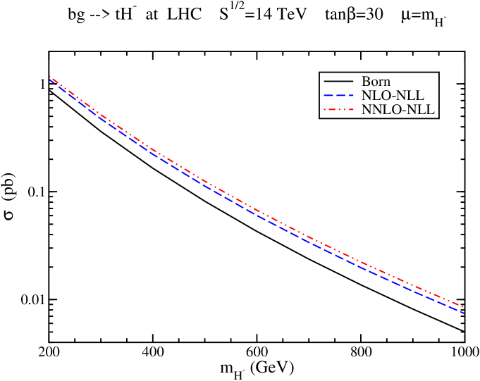
We now turn our attention to detailed numerical results for charged Higgs production at the LHC. In Figure 1 we plot the cross section versus charged Higgs mass for $pp$ collisions at the LHC with $\sqrt{S}=14$ TeV. Here and throughout this paper we use the MRST2002 approximate NNLO parton distributions [27] with the respective three-loop evaluation of $\alpha_{s}$. We set the factorization scale equal to the renormalization scale and denote this common scale by $\mu$. We show results for the Born, NLO-NLL, and NNLO-NLL cross sections, all with a choice of scale $\mu=m_{H^{-}}$. We use the same NNLO parton densities and couplings in all the results, so that we can concentrate on the effects of the soft-gluon corrections. We choose a value $\tan\beta=30$. It is straightforward to get the results for any other value of $\tan\beta$, since the only dependence on $\beta$ in our equations is in the factor $m_{b}^{2}\tan^{2}\beta+m_{t}^{2}\cot^{2}\beta$ appearing in the Born term, Eq. 2.1. The cross sections span over two orders of magnitude in the mass range shown, 200 GeV $\leq m_{H^{-}}\leq$ 1000 GeV. The NLO and NNLO threshold corrections are positive and provide a significant enhancement to the lowest-order result. We note that the cross sections for the related process ${\bar{b}}g\rightarrow{\bar{t}}H^{+}$ are exactly the same.

Figure 2: The $K$-factors for charged Higgs production at the LHC.

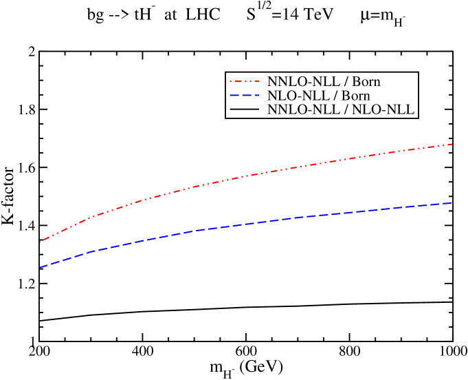
The relative size of the corrections is better shown in Figure 2 where we plot the $K$-factors, i.e. ratios of cross sections at various orders. The NLO-NLL / Born curve shows that the NLO threshold corrections enhance the Born cross section by approximately 25% to 50% depending on the mass of the charged Higgs. As expected the corrections increase for higher charged Higgs masses since then we get closer to threshold. The NNLO-NLL / Born curve shows that if we include the NNLO threshold corrections we get an enhancement over the Born result of approximately 35% to 70% in the range of masses shown. Again the enhancement increases with charged Higgs mass, as expected. Finally, the NNLO-NLL / NLO-NLL curve shows clearly the further enhancement over NLO that the NNLO threshold corrections provide. This curve is simply the ratio of the other two curves and varies between 7% and 14%.

We now want to compare our NLO-NLL results with the exact results that have been derived in [12, 13]. We note that different choices of factorization/renormalization scales were used in those references. In Ref. [12] the reference scale chosen was $m_{H^{-}}+m_{t}$ while in Ref. [13] it was $(m_{H^{-}}+m_{t})/2$. In this paper we choose $m_{H^{-}}$. This is the natural choice in our approach since we are considering logarithms of $s_{4}/m^{2}_{H^{-}}$. Of course any choice of scale is theoretically possible and a cross section known to all orders does not depend on the scale. However a finite-order cross section does depend on the scale, though the dependence decreases as we move from Born to NLO to NNLO and so on. The work in [12, 13] indeed showed a reduction of scale dependence when the NLO corrections are added relative to the Born cross section. In fact, as we will see below, the NNLO threshold corrections further decrease the scale dependence, thus resulting in more stable predictions.

Figure 3: The ratio of cross sections at various scales for charged Higgs production at the LHC. The bold lines are with $\mu=m_{H^{-}}+m_{t}$; the rest are with $\mu=(m_{H^{-}}+m_{t})/2$.

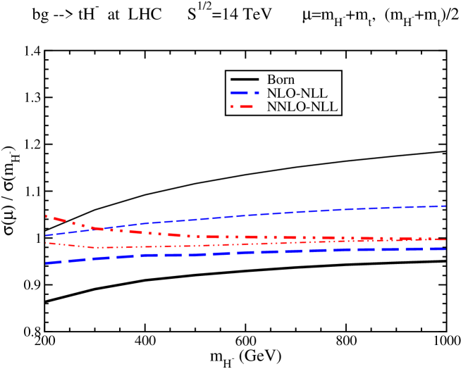
Before comparing our results to the exact NLO cross section, we can check the effect of choosing the scales used in Refs. [12, 13]. In Figure 3 we plot the ratios of the cross sections with choice of reference scale $\mu=m_{H^{-}}+m_{t}$ (bold lines) and $\mu=(m_{H^{-}}+m_{t})/2$ (thin lines) over the cross section with scale $\mu=m_{H^{-}}$. We see that indeed there is a considerable variation at lowest order, but this progressively diminishes at NLO and NNLO. In fact at NNLO there is hardly any difference between the two lines at large values of the charged Higgs mass. Thus we see the stabilization of the cross section versus scale variation when higher-order corrections are included. We will say more regarding this important point and show more plots below.

Figure 4: The ratio of exact and approximate NLO cross sections for charged Higgs production at the LHC.

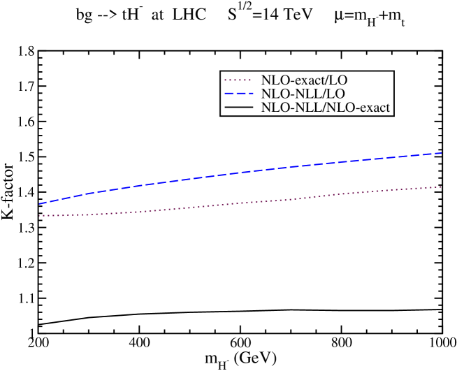
We now compare the NLO soft-gluon results with the exact NLO cross section. In Figure 4, we compare the NLO-NLL cross section with the exact NLO cross section of reference [12]. To make the comparison, the NLO-NLL result is calculated here for $\mu=m_{H^{-}}+m_{t}$ since that’s the scale chosen in [12] and also using a two-loop $\alpha_{s}$. Also, to remove discrepancies arising from different choices of parton distribution functions, we plot $K$-factors. The NLO-exact / LO curve is taken from Ref. [12] by dividing curve 1 by curve 2 in Figure 6 of that reference (to account for the different definition of $K$-factor used there). The fact that the NLO-NLL / NLO-exact curve is very close to 1 (only a few percent difference) shows that the NLO-NLL cross section is a remarkably good approximation to the exact NLO result. As noted before, we might have expected this on theoretical grounds since this is near-threshold production, and also from prior experience with many other near-threshold hard-scattering cross sections [18, 19, 20, 21, 22].

Figure 5: The scale dependence for production of a charged Higgs with mass $m_{H^{-}}=500$ GeV at the LHC.

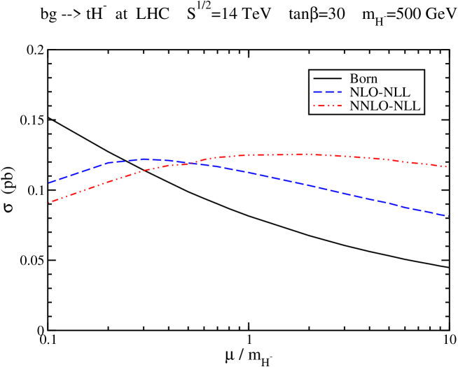
In Figure 5, we plot the scale dependence of the cross section for a fixed charged Higgs mass $m_{H^{-}}=500$ GeV and $\tan\beta=30$. We plot a large range in scale, $0.1\leq\mu/m_{H^{-}}\leq 10$, and see indeed that the threshold corrections greatly decrease the scale dependence of the cross section. The NNLO-NLL curve is relatively flat.

Figure 6: The scale dependence for charged Higgs production at the LHC. The bold lines are with $\mu=2m_{H^{-}}$; the rest are with $\mu=m_{H^{-}}/2$.

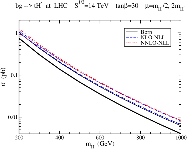
In Figure 6 we plot the the cross section as a function of charged Higgs mass with two different choices of scale, $\mu=m_{H^{-}}/2$ and $2m_{H^{-}}$. We see that the variation with scale of the Born cross section is quite large. The variation at NLO-NLL is smaller, and at NNLO-NLL it is very small. In fact the two NNLO-NLL curves are on top of each other for most of the range in $m_{H^{-}}$. Hence, the scale dependence of the cross section is drastically reduced when higher-order corrections are included. This is as expected from and is consistent with the reduced scale dependence shown in Figures 3 and 5.

Figure 7: The $\tan\beta$ dependence for charged Higgs production at the LHC.

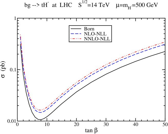
In Figure 7 we plot the dependence of the cross section on $\tan\beta$, over the range $1\leq\tan\beta\leq 50$, for fixed charged Higgs mass and scale $\mu=m_{H^{-}}=500$ GeV. The cross section is at a minimum near $\tan\beta=8$. We note that the $\tan\beta$ dependence arises in the factor $m_{b}^{2}\tan^{2}\beta+m_{t}^{2}\cot^{2}\beta$ in the Born term and thus the shape of the curves at higher orders is similar. The dependence on $\tan\beta$ is quite large, spanning nearly two orders of magnitude in the range shown.

Figure 8: The top quark mass dependence for charged Higgs production at the LHC.

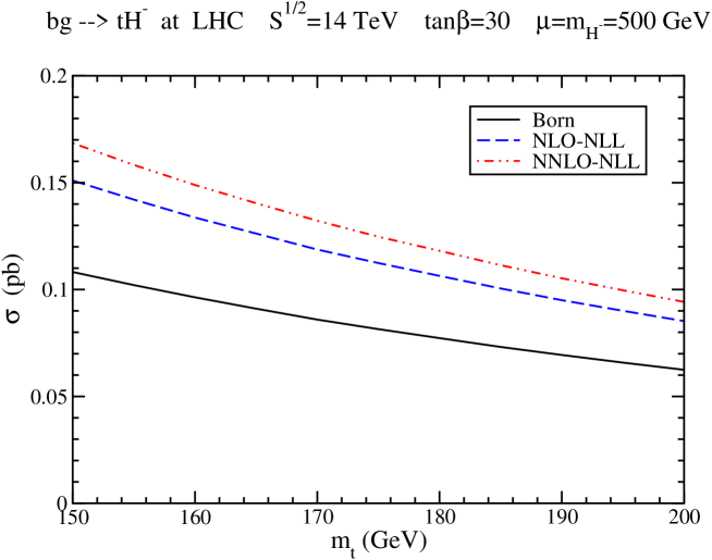
In Figure 8 we plot the dependence of the cross section on the top quark mass for fixed charged Higgs mass and scale $\mu=m_{H^{-}}=500$ GeV and $\tan\beta=30$. We see that the dependence is not very strong so that the present experimental uncertainties on the top quark mass do not play a dominant role in the total uncertainty of the charged Higgs production cross section. As the top quark mass gets more precisely known, this dependence will diminish further.

4 Conclusion

The process $bg\rightarrow tH^{-}$ offers a promising possibility for discovering a charged Higgs boson. Charged Higgs production at the LHC receives important contributions from the threshold region. The NLO corrections to the process $bg\rightarrow tH^{-}$ are quite large. We have seen that the full NLO cross section is very well approximated by the NLO-NLL soft-gluon result, to within a few percent. The NNLO soft-gluon threshold corrections to charged Higgs production are important and further stabilize the cross section versus changes in factorization and renormalization scales. The dependence on $\tan\beta$ and on the charged Higgs mass are quite large while the dependence on the top quark mass is milder.

References

- [1] A.C. Bawa, C.S. Kim, and A.D. Martin, Z. Phys. C 47, 75 (1990).
- [2] J.F. Gunion, Phys. Lett. B 322, 125 (1994).
- [3] V.D. Barger, R.J.N. Phillips, and D.P. Roy, Phys. Lett. B 324, 236 (1994).
- [4] C.S. Huang and S.H. Zhu, Phys. Rev. D 60, 075012 (1999).
- [5] K. Odagiri, Phys. Lett. B 452, 327 (1999).
- [6] F. Borzumati, J.L. Kneur, and N. Polonsky, Phys. Rev. D 60, 115011 (1999).
- [7] D.P. Roy, Phys. Lett. B 459, 607 (1999).
- [8] S. Moretti and D.P. Roy, Phys. Lett. B 470, 209 (1999).
- [9] L.G. Jin, C.S. Li, R.J. Oakes, and S.H. Zhu, Eur. Phys. J. C 14, 91 (2000); Phys. Rev. D 62, 053008 (2000).
- [10] A. Belyaev, D. Garcia, J. Guasch, and J. Sola, Phys. Rev. D 65, 031701 (2002); JHEP 06, 059 (2002).
- [11] G.P. Gao, G.R. Lu, Z.H. Xiong, and J.M. Yang, Phys. Rev. D 66, 015007 (2002).
- [12] S.H. Zhu, Phys. Rev. D 67, 075006 (2003).
- [13] T. Plehn, Phys. Rev. D 67, 014018 (2003).
- [14] E.L. Berger, T. Han, J. Jiang, and T. Plehn, hep-ph/0312286.
- [15] N. Kidonakis, Mod. Phys. Lett. A 19, 405 (2004);
- [16] The Higgs Working Group: Summary Report, in Les Houches 2003, hep-ph/0406152.
- [17] N. Kidonakis, in DIS 2004, hep-ph/0406179.
- [18] N. Kidonakis, Phys. Rev. D 64, 014009 (2001); Int. J. Mod. Phys. A 16 Suppl. 1A, 363 (2001), hep-ph/0009013; N. Kidonakis and R. Vogt, Phys. Rev. D 68, 114014 (2003); Eur. Phys. J. C 33, s466 (2004), hep-ph/0309045; Eur. Phys. J. C 36, 201 (2004); in DPF 2004, hep-ph/0410367.
- [19] N. Kidonakis and A. Sabio Vera, JHEP 02, 027 (2004); in DPF 2004, hep-ph/0409206; hep-ph/0409337.
- [20] N. Kidonakis and J.F. Owens, Phys. Rev. D 61, 094004 (2000); Int. J. Mod. Phys. A 19, 149 (2004); N. Kidonakis, in EPS-HEP 99, p. 392, hep-ph/9910240.
- [21] N. Kidonakis and J.F. Owens, Phys. Rev. D 63, 054019 (2001).
- [22] A. Belyaev and N. Kidonakis, Phys. Rev. D 65, 037501 (2002); N. Kidonakis and A. Belyaev, JHEP 12, 004 (2003); in DIS 2004, hep-ph/0407032.
- [23] N. Kidonakis and G. Sterman, Phys. Lett. B 387, 867 (1996); Nucl. Phys. B 505, 321 (1997); N. Kidonakis, G. Oderda, and G. Sterman, Nucl. Phys. B 525, 299 (1998); Nucl. Phys. B 531, 365 (1998); N. Kidonakis, Int. J. Mod. Phys. A 15, 1245 (2000).
- [24] E. Laenen, G. Oderda, and G. Sterman, Phys. Lett. B 438, 173 (1998).
- [25] N. Kidonakis, Int. J. Mod. Phys. A 19, 1793 (2004); in DPF 2004, hep-ph/0410116.
- [26] A. Djouadi, J. Kalinowski, and M. Spira, Comput. Phys. Commun. 108, 56 (1998).
- [27] A.D. Martin, R.G. Roberts, W.J. Stirling, and R.S. Thorne, Eur. Phys. J. C 28, 455 (2003).