Soft data and the hard pomeron

Abstract

We show that the introduction of an additional, hard, singularity in soft forward amplitudes enables one to improve considerably the fits using a simple-pole structure for the soft pomeron.

1 Introduction

One of the central questions in QCD concerns the continuation of short-distance results to the soft region or, in other words, the extension of the large-$Q^{2}$ perturbative description of the data ($F_{2}$, $F_{2}^{c}$,…) to the non-perturbative $Q^{2}=0$ domain ($\sigma_{tot}$, $\rho$). There are several phenomenological models that already attempt to describe such a transition [1, 2]. Most of them assume a rise in total cross sections proportional to $\log^{2}(s/s_{0})$, which describes best the data, both for $\sigma_{tot}$ and $\rho$ [3]. Such a behaviour in $s$ $-$ or $1/x$ $-$ can be used as an initial condition for evolution equations [4], and is even a very good approximation to the result of the evolution [5]. Such a rise can be obtained via a strong unitarisation of a BFKL-like singularity [2].

Following [6], we want here to explore another possibility: we shall assume that “bare” exchanges of Regge trajectories account for most of the elastic amplitude, and that unitarisation and cuts have a small, negligible, effect. This is the standard assumption that lead Donnachie and Landshoff [7] to a very simple and successful description of soft scattering, based on the exchange of two degenerate leading meson trajectories and of a soft pomeron. Recently, it was however found that such a simple singularity structure does not allow a good description neither of soft forward data [3] nor of $F_{2}$. In the latter case, Donnachie and Landshoff [8] have shown that the introduction of a second pomeron with a large intercept $\alpha_{h}\approx 1.4$ is consistent both with the evolution equations and with the data. We want here to address the former question, and show that the introduction of the $same$ hard singularity makes the fit to $\sigma_{tot}$ and $\rho$ as good as that based one a $\log^{2}(s/s_{0})$ rise.

2 Improved analysis

Figure 1: Difference between $\rho$ values fitted with (plain) and without (dashed) a hard pomeron, assuming all singularities are simple poles.

In the analysis of ref. [3], models based on a simple-pole pomeron were dismissed mainly because they could not describe the real part of the amplitude well, or equivalently because the fit to $\rho$, the ratio of the real part to the imaginary part of the elastic hadronic amplitude, had an unacceptably high $\chi^{2}$. Hence we have improved the treatment of the real part of the amplitude by introducing the following refinements:
$\bullet$ We include and fit the subtraction constant present in the real part of the amplitude because of rising $C=+1$ contributions;
$\bullet$ We use integral dispersion relations down to the correct threshold and, at low energies (for which the analytic asymptotic model is not correct), we use (a smooth fit to) the data for $\sigma_{tot}$ to perform the dispersion integral.
$\bullet$ We use the exact form of the flux factor ${\cal F}=2m_{p}p_{lab}$ and Regge variables $\tilde{s}\equiv{s-u\over 2}$ proportional to $\cos(\theta_{t})$ instead of their dominant terms at large-$s$.

Following [3], we fit total cross sections and $\rho$ for $pp$, $\bar{p}p$, $\pi^{\pm}p$ and $K^{\pm}p$, and total cross sections for $\gamma p$ and $\gamma\gamma$ in the region 5 GeV $\leq\sqrt{s}$. Furthermore, as we are using simple poles, we use Gribov-Pomeranchuk factorisation of the residues at each simple pole to predict the $\gamma\gamma$ amplitude from the $pp$ and $\gamma p$ data [9].

If we define the hadronic $ab$ amplitude as ${\cal A}_{ab}={\Re}_{ab}+i{\Im}_{ab}$, we obtain the total cross section as

$$\sigma_{tot}^{ab}\equiv\frac{1}{2m_{b}p_{lab}}\,\Im^{ab}$$ (1)

with $p_{lab}$ the momentum of particle $b$ in the $a$ rest frame. The real part of the amplitude can then be obtained from integral dispersion relations:

$$\Re_{ab} = R_{ab}$$ (2)

$$+ \frac{E}{\pi}\ {\textrm{P}}\int_{m_{a}}^{\infty}\left[\frac{\Im_{ab}}{E^{\prime}-E}-\frac{\Im_{a\bar{b}}}{E^{\prime}+E}\right]\,{dE^{\prime}\over E^{\prime}},$$

where $E$ is the energy of $b$ in the rest frame of $a$, P indicates that we have to do a principal-part integral, and $R_{ab}$ is the subtraction constant.

The models that we consider are defined by the following equation:

$${\Im}_{ab}\equiv s_{1}\left[{\Im}^{R+}_{ab}\left({\tilde{s}\over s_{1}}\right)+{\Im}^{S}_{ab}\left({\tilde{s}\over s_{1}}\right)\mp{\Im}^{-}_{ab}\left({\tilde{s}\over s_{1}}\right)\right],$$ (3)

with $s_{1}=1$ GeV², and the $-$ sign in the last term for particles. For the two reggeon contributions, we use simple-pole expressions ${\Im}^{R+}_{pb}=P_{b}\left({\tilde{s}\over s_{1}}\right)^{\alpha_{+}}$ and ${\Im}^{-}_{pb}=M_{b}\left({\tilde{s}\over s_{1}}\right)^{\alpha_{-}}$. For the pomeron contribution, we allow two simple poles to contribute:

$$\Im^{S}_{pb}=S_{b}\left({\tilde{s}\over s_{1}}\right)^{\alpha_{o}}+H_{b}\left({\tilde{s}\over s_{1}}\right)^{\alpha_{h}}$$ (4)

For comparison, we also consider expressions corresponding to a dipole or a tripole:

$$\Im^{S}_{pb}=D_{b}{\tilde{s}\over s_{1}}\ln\frac{\tilde{s}}{s_{d}},$$ (5)

$$\Im^{S}_{pb}=T_{b}{\tilde{s}\over s_{1}}\left[\ln^{2}\frac{\tilde{s}}{s_{t}}+t^{\prime}_{b}\right].$$ (6)

Figure 2: Fit to the $\gamma\gamma$ total cross section using Gribov-Pomeranchuk factorisation.

3 Results

The improved treatment of $\rho$ leads to a better fit in all cases (a dipole pomeron (5) reaches a $\chi^{2}/dof$ of 0.94 and a tripole pomeron (6) one of 0.93, whereas they were both 0.98 in the standard analysis [3]). However, if we use only one simple pole for the pomeron ($i.e.$ if we set $H_{b}=0$ in (4), we still cannot get a fit comparable to those obtained using (5, 6).  

Parameters	value
$\alpha_{h}$	1.45 $\pm$ 0.01
$H_{p}$	0.10 $\pm$ 0.02
$H_{\pi}$	0.28 $\pm$ 0.03
$H_{K}$	0.30 $\pm$ 0.03
$H_{\gamma}$	0.0006 $\pm$ 0.0002
$\alpha_{o}$	1.0728 $\pm$ 0.0008
$S_{p}$	56.2 $\pm$ 0.3
$S_{\pi}$	32.7 $\pm$ 0.2
$S_{K}$	28.3 $\pm$ 0.2
$S_{\gamma}$	0.174 $\pm$ 0.002
$\alpha_{+}$	0.608 $\pm$ 0.003
$P_{p}$	158 $\pm$ 2
$P_{\pi}$	78 $\pm$ 1
$P_{K}$	46 $\pm$ 1
$P_{\gamma}$	0.28 $\pm$ 0.01
$\alpha_{-}$	0.473 $\pm$ 0.008
$M_{p}$	79 $\pm$ 3
$M_{\pi}$	14.2 $\pm$ 0.5
$M_{K}$	32 $\pm$ 1
$R_{pp}$	-164 $\pm$ 33
$R_{p\pi}$	-96 $\pm$ 21
$R_{pK}$	3 $\pm$ 26

Table 1
Parameters obtained in the fit from 5 to 100 GeV.  

However, we found that the inclusion of the second singularity in (4) has a dramatic effect: the $\chi^{2}$ drops from 661 to 551 for 619 points, nominally a 10 $\sigma$ effect! More surprisingly, the new singularity has an intercept of 1.39, very close to that obtained in DIS by Donnachie and Landshoff. However, as was already known [10], the new trajectory, which we shall call the hard pomeron, almost decouples from $pp$ and $\bar{p}p$ scattering. Nevertheless, it improves considerably the description of $\pi p$ and $Kp$ amplitudes, and parametrisation (4) becomes as good as (6).

The decoupling in $pp$ and $\bar{p}p$ scattering can easily be understood: any sizable coupling will produce a dramatic rise with $s$, and only $pp$ and $\bar{p}p$ data reach high energy. For these data, the hard pomeron contribution will surely need to be unitarised (see however [11] for a different opinion). To get a handle on the hard pomeron parameters, it is thus a good idea to fit to lower energies first. We choose to consider the region from 5 to 100 GeV (which includes all the $\pi p$ and $Kp$ data). We checked that the parameters describing the hard pomeron component are stable if we slightly change the region of interest, by augmenting the minimum energy to $e.g.$ 10 GeV, or by decreasing the maximum energy to $e.g.$ 40 GeV.

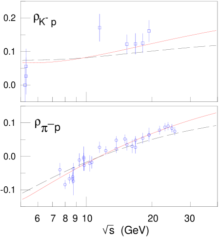
Hence our best estimate for the parameters describing the hard pomeron is shown in Table 1, and some of the fits are shown in Fig. 1.

As can be seen, the parameters are in agreement with those describing DIS, although the soft pomeron is a bit softer than assumed in [8]. In particular, we obtain for the hard-pomeron singularity

$$\alpha_{h}=1.45\pm 0.01.$$ (7)

However, a new and unexpected hierarchy of couplings is needed. Writing $H_{ab}=h_{a}\ h_{b}$, we obtain:

$$1\approx h_{K}\approx 1.1h_{\pi}\approx 3.2h_{p}$$ (8)

Such a hierarchy may be expected in dipole models [1], but it is stronger than expected. Size effects may thus not be sufficient to account for it.

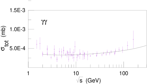
The hard pomeron is probably not a simple pole, but it must be close to it: as we obtain the $\gamma\gamma$ cross section via Gribov-Pomeranchuk factorisation, we indeed test the analytic nature of the singularity [9]. The result is shown in Fig. 2. One can see that the LEP data are compatible with our results, and that we prefer a lower value, such as that obtained using PHOJET. Also, our value of the coupling of the hard pomeron to protons must be an upper limit: bigger values would lead to too small a $\gamma\gamma$ cross section.

Figure 3: Relative contribution of the various terms of the amplitude, compared with the $C=+1$ part of the amplitude (“tot”) in the $pp$ case. The dashed curve is for a hard pole, and the plain curves for the unitarised form.

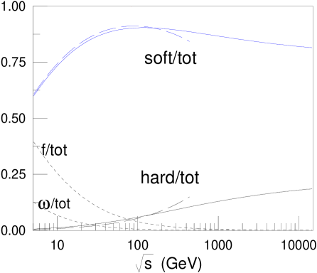
To obtain a fit to higher energies, one must surely unitarise the hard pomeron contribution, as it violates the black-disk limit around $\sqrt{s}=400$ GeV. The way to do this is far from clear, especially as there can be some mixing with the other trajectories. We have shown in [6] that it is possible to find a unitarisation scheme which produces a good description of the data for all energies. Its contribution, shown in Fig. 3, is always smaller than 25% of the total cross section.

4 Outlook

In conclusion, we have shown [6] that it is possible that the hard pomeron is present in soft data and that this object may be similar to a simple pole for $\sqrt{s}\leq 100$ GeV. This means that the bulk of the simple-pole phenomenology can be kept in the presence of a hard pomeron. The latter however will bring corrections at large $s$, large $Q^{2}$ or large $t$. The surprising hierarchy of couplings (8), as well as the smallness of the residues, indicates that our results will need confirmation. It may be worth noting here that we obtain similar results if we exclude the $\rho$ data from the analysis. Also, some evidence for a hard pomeron may also be found in elastic scattering data [12].

References

- [1] A. Donnachie and H. G. Dosch, Phys. Rev. D 65 (2002) 014019 [arXiv:hep-ph/0106169];
- [2] N. N. Nikolaev, J. Speth, V.R. Zoller, Phys. Lett. B 473 (2000) 157; J. Bartels, E. Gotsman, E. Levin, M. Lublinsky and U. Maor, Phys. Lett. B 556 (2003) 114; S. M. Troshin and N. E. Tyurin, Phys. Part. Nucl. 30 (1999) 550.
- [3] J. R. Cudell et al. [COMPETE Collaboration], Phys. Rev. D 65 (2002) 074024 [arXiv:hep-ph/0107219]; Phys. Rev. Lett. 89 (2002) 201801 [arXiv:hep-ph/0206172]; K. Hagiwara et al. [Particle Data Group Collaboration], Phys. Rev. D 66 (2002) 010001.
- [4] G. Soyez, arXiv:hep-ph/0407098; Phys. Rev. D 67 (2003) 076001 [arXiv:hep-ph/0211361]. L. Csernai, L. Jenkovszky, K. Kontros, A. Lengyel, V. Magas and F. Paccanoni, Eur. Phys. J. C 24 (2002) 205 [arXiv:hep-ph/0112265].
- [5] G. Soyez, Phys. Rev. D 69 (2004) 096005 [arXiv:hep-ph/0306113]; J. R. Cudell and G. Soyez, Phys. Lett. B 516 (2001) 77 [arXiv:hep-ph/0106307].
- [6] J. R. Cudell, E. Martynov, O. Selyugin and A. Lengyel, Phys. Lett. B 587 (2004) 78 [arXiv:hep-ph/0310198].
- [7] A. Donnachie and P. V. Landshoff, Phys. Lett. B 296 (1992) 227 [arXiv:hep-ph/9209205].
- [8] A. Donnachie and P. V. Landshoff, Phys. Lett. B 550 (2002) 160 [arXiv:hep-ph/0204165]; Phys. Lett. B 533 (2002) 277 [arXiv:hep-ph/0111427]; Phys. Lett. B 518 (2001) 63 [arXiv:hep-ph/0105088]; J. R. Cudell, A. Donnachie and P. V. Landshoff, Phys. Lett. B 448 (1999) 281 [Erratum-ibid. B 526 (2002) 413] [arXiv:hep-ph/9901222].
- [9] J. R. Cudell, E. Martynov and G. Soyez, Nucl. Phys. B 682 (2004) 391 [arXiv:hep-ph/0207196].
- [10] J. R. Cudell, V. Ezhela, K. Kang, S. Lugovsky and N. Tkachenko, Phys. Rev. D 61 (2000) 034019 [Erratum-ibid. D 63 (2001) 059901] [arXiv:hep-ph/9908218].
- [11] A. Donnachie and P. V. Landshoff, Phys. Lett. B 595 (2004) 393. [arXiv:hep-ph/0402081].
- [12] J.R. Cudell and E. Martynov, in preparation.