LAL 04-10

Isospin constraints from/on Bππ𝐵𝜋𝜋B\to\pi\pi


M. Pivka𝑎{}^{\,a} and F.R. Le Diberderb𝑏{}^{\,b}

a CERN, PH Department
CH-1211 Geneva 23, Switzerland

b Laboratoire de l’Accélérateur Linéaire,
IN2P3-CNRS et Université de Paris-Sud, F-91898 Orsay, France

Abstract

The Standard Model constraints on α𝛼\alpha which can be derived from the Bππ𝐵𝜋𝜋B\rightarrow\pi\pi decays are revisited in some depth. As experimental inputs, the B0π+πsuperscript𝐵0superscript𝜋superscript𝜋B^{0}\rightarrow\pi^{+}\pi^{-}, B+π+π0superscript𝐵superscript𝜋superscript𝜋0B^{+}\rightarrow\pi^{+}\pi^{0} decays complemented by the B0π0π0superscript𝐵0superscript𝜋0superscript𝜋0B^{0}\rightarrow\pi^{0}\pi^{0} decays, the CP parameters Sππsubscript𝑆𝜋𝜋S_{\pi\pi} and Cππsubscript𝐶𝜋𝜋C_{\pi\pi}, and/or the value of α𝛼\alpha as determined by the global CKM fit are used. The constraints discussed here are model independent in the sense that they rely only on Isospin symmetry, following the Gronau-London proposal. A new bound on 00superscript00{\cal B}^{00} and the function C00(00)subscript𝐶00superscript00C_{00}({\cal B}^{00}) are introduced. While another bound applied to BABAR results is shown to imply that cos(2αeff)2subscript𝛼eff\cos(2\alpha_{\rm eff}) is negative. The Grossman-Quinn bound is rediscussed. A close form expression is given for α𝛼\alpha as a function of the measurements. Various scenarii for the future of the isospin analysis are explored. To probe the Standard Model the (00,C00)superscript00subscript𝐶00({\cal B}^{00},C_{00}) plane is introduced.


1 Introduction

The purpose of this note is to revisit the Standard Model constraints which can be derived from (and on) the Bππ𝐵𝜋𝜋B\rightarrow\pi\pi decays following the Gronau-London proposal [1]. Much have been written already on this topic, for example [2, 3, 4], but fresh developments are presented here.

This study leads to correct a strong bias: the Bππ𝐵𝜋𝜋B\rightarrow\pi\pi isospin analysis is not doomed neither to wait for ultra high luminosity, nor to have a small branching ratio 00superscript00{\cal B}^{00} (corresponding to the B0π0π0superscript𝐵0superscript𝜋0superscript𝜋0B^{0}\rightarrow\pi^{0}\pi^{0} decay) to be able to constrain α𝛼\alpha. The current period of time is very exciting: anything can happen in the next three years, including a rather precise determination of α𝛼\alpha.

In Section 2 is recalled the present experimental status: the values of the three branching ratios (+=(B0π+π)superscriptabsentsuperscript𝐵0superscript𝜋superscript𝜋{\cal B}^{+-}={\cal B}(B^{0}\to{\pi^{+}\pi^{-}}), +0=(B+π+π0)superscript0superscript𝐵superscript𝜋superscript𝜋0{\cal B}^{+0}={\cal B}(B^{+}\to\pi^{+}\pi^{0}) and 00superscript00{\cal B}^{00}) and the two time-dependent asymmetry parameters (Sππsubscript𝑆𝜋𝜋S_{\pi\pi} and Cππsubscript𝐶𝜋𝜋C_{\pi\pi}). The statistical meaning of the BABAR and Belle results for Sππsubscript𝑆𝜋𝜋S_{\pi\pi} and Cππsubscript𝐶𝜋𝜋C_{\pi\pi} is discussed, considering two different statistical treatments.

In Section 3, the plague of the mirror solutions is explicited. Section 4 then turns to some algebra. A new bound on 00superscript00{\cal B}^{00} is presented Eq.(24), from which the sign of cos(2αeff)2subscript𝛼eff\cos(2\alpha_{\rm eff}) is inferred, a function C00(00)subscript𝐶00superscript00C_{00}({\cal B}^{00}) is explicited Eq.(35), a close form expression for α𝛼\alpha as a function of the measurements is given, and the meaning of the Grossman-Quinn bound on ααeffdelimited-∣∣𝛼subscript𝛼eff\mid\alpha-\alpha_{\rm eff}\mid is discussed.

In Section 5 the perspectives for measuring α𝛼\alpha are pondered. First an exploration of the space of still open possibilities is attempted. Then two scenarii for the high luminosity regime (10ab110superscriptab110~{}\mbox{ab}^{-1}) are considered. For the sake of completeness a nasty and a nice scenario are considered, with 500fb1500superscriptfb1500~{}\mbox{fb}^{-1}.

The analysis is reconsidered from another point of view in Section 6. Instead of the usual ρ¯¯𝜌\bar{\rho} and η¯¯𝜂\bar{\eta} variables, the branching ratio 00superscript00{\cal B}^{00} and the asymmetry term C00subscript𝐶00C_{00} are taken as key variables to probe the Standard Model, when dealing with Bππ𝐵𝜋𝜋B\rightarrow\pi\pi decays. The present experimental status and the high luminosity potential are discussed in this context.

The ElectroWeak Penguin complications are neglected throughout the note, having in mind that, when accounted for, they should not utterly blur the picture.

The effects of radiative corrections [5, 6], which imply a 555 to 10%percent1010\% increase on the published branching ratios are not taken into account in the present analysis.

2 Comparison of BABAR and Belle results

The two detectors BABAR and Belle located respectively at the asymmetric B𝐵B Factory PEP-II and KEK-B measure branching ratios and time-dependent asymmetries for the Bππ𝐵𝜋𝜋B\to\pi\pi decays. If the BABAR values, for the time-dependent asymmetries, are in the physical region, Belle ones are not. A special statistical treatment is then advised to deal with such a situation where a measurement lies beyond the physical boundaries: this is the purpose of this section. First are recalled in Section 2.1 the values measured by BABAR and Belle. The world average (W.A.) ones are given as well [7]. Section 2.2 discusses the results using the standard statistical treatment. Section 2.3 turns to the boundary effect via a particular treatment.

2.1 Present experimental status

The most recent values of BABAR and Belle are summarized in Table 1. All branching ratios are quoted in the 106superscript10610^{-6} unit, as in the whole document. For the world average values of the two time-dependent asymmetries terms Sππsubscript𝑆𝜋𝜋S_{\pi\pi} and Cππsubscript𝐶𝜋𝜋C_{\pi\pi}, the discrepancy between BABAR and Belle is not taken into account and the results are merged together at face values. That is to say the raw measurements are taken, without accounting for the fact that physical values should be in the disk Sππ2+Cππ21superscriptsubscript𝑆𝜋𝜋2superscriptsubscript𝐶𝜋𝜋21S_{\pi\pi}^{2}+C_{\pi\pi}^{2}\leq 1. Since Belle results are outside the physical disk, in some instances modified and fictitious results are used instead, where the Belle measurements are forced back onto the unity circle: they are denoted Belle in the present document.

+(106)superscriptabsentsuperscript106{\cal B}^{+-}~{}(10^{-6}) +0(106)superscript0superscript106{\cal B}^{+0}~{}(10^{-6}) 00(106)superscript00superscript106{\cal B}^{00}~{}(10^{-6}) Cππsubscript𝐶𝜋𝜋C_{\pi\pi} Sππsubscript𝑆𝜋𝜋S_{\pi\pi} ρ𝜌\rho
BABAR 4.7±0.6plus-or-minus4.70.64.7\ \pm 0.6\ 5.5±1.2plus-or-minus5.51.25.5\ \pm 1.2\ 2.1±0.7plus-or-minus2.10.72.1\ \pm 0.7\ 0.19±0.20plus-or-minus0.190.20-0.19\pm 0.20 0.40±0.22plus-or-minus0.400.22-0.40\pm 0.22 0.020.02-0.02
Belle 4.4±0.7plus-or-minus4.40.74.4\ \pm 0.7\ 5.0±1.3plus-or-minus5.01.35.0\ \pm 1.3\ 1.7±0.6plus-or-minus1.70.61.7\ \pm 0.6\ 0.58±0.17plus-or-minus0.580.17-0.58\pm 0.17 1.00±0.22plus-or-minus1.000.22-1.00\pm 0.22 0.290.29-0.29
Belle - - - 0.55±0.17plus-or-minus0.550.17-0.55\pm 0.17 0.84±0.22plus-or-minus0.840.22-0.84\pm 0.22 -
W.A. 4.55±0.44plus-or-minus4.550.444.55\pm 0.44 5.18±0.77plus-or-minus5.180.775.18\pm 0.77 1.9±0.5plus-or-minus1.90.51.9\ \pm 0.5\ 0.46±0.13plus-or-minus0.460.13-0.46\pm 0.13 0.73±0.16plus-or-minus0.730.16-0.73\pm 0.16 0.170.17-0.17
Table 1: Input values to the fits for the branching ratios [8, 9, 10, 11] and for the CP violating asymmetries [12, 13]. The notation Belle refers to the Belle results for the branching ratios, but where the measured values for Sππsubscript𝑆𝜋𝜋S_{\pi\pi} and Cππsubscript𝐶𝜋𝜋C_{\pi\pi} are replaced by the values quoted by Belle for Sππbestsuperscriptsubscript𝑆𝜋𝜋bestS_{\pi\pi}^{\rm best} and Cππbestsuperscriptsubscript𝐶𝜋𝜋bestC_{\pi\pi}^{\rm best} (Section 2.3). The world average branching ratios are obtained using in addition CLEO results [14].

2.2 The unbounded (standard) statistical treatment

A proper method to compute a confidence level (CL) associated to a given theoretical hypothesis (hyp) and an experimental result (exp) is the following: one defines a test statistics w(hyp,exp)𝑤hypexpw({\rm hyp},{\rm exp}) which bears the property that the larger its value, the smaller the likelihood of the hypothesis (hyp) to be true, given the experimental result (exp). One denotes fhyp(w)subscript𝑓hyp𝑤f_{{\rm hyp}}(w) the probability density function of the variable w𝑤w, the hypothesis being assumed to be true. The confidence level is then computed as:

CL(hyp,exp)=w(hyp,exp)fhyp(w)𝑑w.CLhypexpsuperscriptsubscript𝑤hypexpsubscript𝑓hyp𝑤differential-d𝑤{\rm CL}({\rm hyp},{\rm exp})~{}=~{}\int_{w({\rm hyp},{\rm exp})}^{\infty}f_{{\rm hyp}}(w)dw~{}. (1)

When the theoretical hypothesis is unbounded, a standard treatment is to identify w𝑤w with the χ2superscript𝜒2\chi^{2} measuring the agreement between theory and experiment. When the theoretical hypothesis is bounded, this standard treatment is still valid. However, it suffers from a drawback: if, because of a statistical fluctuation, the experimental result lies far away from the allowed region, the confidence level might be very small, whatever the hypothesis. The underlying theory is therefore ruled out. The drawback stems from the fact that one may wish to set a confidence level assuming that the underlying theory is true. That is to say, one does not question the validity of the theory as a whole, but one is interested to reach a statement on some of its theoretical parameters.

2.3 The bounded statistical treatment

The standard, χ2superscript𝜒2\chi^{2}-based, statistical analysis of the Sππsubscript𝑆𝜋𝜋S_{\pi\pi} and Cππsubscript𝐶𝜋𝜋C_{\pi\pi} measurements may lead to the exclusion of the whole physical domain Sππ2+Cππ21superscriptsubscript𝑆𝜋𝜋2superscriptsubscript𝐶𝜋𝜋21S_{\pi\pi}^{2}+C_{\pi\pi}^{2}\leq 1 if statistical fluctuations bring the measurements far enough outside it. Because Belle values enter deep into the unphysical region, the hypothesis of no CP violation in the Bππ𝐵𝜋𝜋B\rightarrow\pi\pi (Sππ=Cππ=0subscript𝑆𝜋𝜋subscript𝐶𝜋𝜋0S_{\pi\pi}=C_{\pi\pi}=0) is ruled out at 2.48×10⁵%2.48percentsuperscript1052.48\times 10^{-5}\% CL by her analysis [13]. Here is presented a statistical treatment which by construction cannot rule out the whole physical domain. It incorporates the (mild) assumption that at least Quantum Mechanics is right and hence that Sππ2+Cππ21superscriptsubscript𝑆𝜋𝜋2superscriptsubscript𝐶𝜋𝜋21S_{\pi\pi}^{2}+C_{\pi\pi}^{2}\leq 1.

Let us denote:

  • Sππhypsuperscriptsubscript𝑆𝜋𝜋hypS_{\pi\pi}^{\rm hyp} and Cππhypsuperscriptsubscript𝐶𝜋𝜋hypC_{\pi\pi}^{\rm hyp} , the theoretical values one would like to set a CL on. They are within the physical domain in the (Sππ,Cππ)subscript𝑆𝜋𝜋subscript𝐶𝜋𝜋(S_{\pi\pi},C_{\pi\pi}) plane,

  • Sππexpsuperscriptsubscript𝑆𝜋𝜋expS_{\pi\pi}^{\rm exp} and Cππexpsuperscriptsubscript𝐶𝜋𝜋expC_{\pi\pi}^{\rm exp} , the measured values. They can be anywhere in the (Sππ,Cππ)subscript𝑆𝜋𝜋subscript𝐶𝜋𝜋(S_{\pi\pi},C_{\pi\pi}) plane,

  • Sππbestsuperscriptsubscript𝑆𝜋𝜋bestS_{\pi\pi}^{\rm best} and Cππbestsuperscriptsubscript𝐶𝜋𝜋bestC_{\pi\pi}^{\rm best} , the theoretical values which are in the best agreement with the above measurements. They are within the physical domain in the (Sππ,Cππ)subscript𝑆𝜋𝜋subscript𝐶𝜋𝜋(S_{\pi\pi},C_{\pi\pi}) plane. These values are the ones used to replace Sππexpsuperscriptsubscript𝑆𝜋𝜋expS_{\pi\pi}^{\rm exp} and Cππexpsuperscriptsubscript𝐶𝜋𝜋expC_{\pi\pi}^{\rm exp}, when considering the Belle results,

  • χ2(exp|hyp)superscript𝜒2conditionalexphyp\chi^{2}({\rm exp}|{\rm hyp}) is the χ2superscript𝜒2\chi^{2} one gets when comparing the measured values with the hypotheses Sππhypsuperscriptsubscript𝑆𝜋𝜋hypS_{\pi\pi}^{\rm hyp} and Cππhypsuperscriptsubscript𝐶𝜋𝜋hypC_{\pi\pi}^{\rm hyp},

  • χ2(exp|best)superscript𝜒2conditionalexpbest\chi^{2}({\rm exp}|{\rm best}) is the minimal χ2(exp|hyp)superscript𝜒2conditionalexphyp\chi^{2}({\rm exp}|{\rm hyp}) one gets when exploring the physical domain. The corresponding values of Sππsubscript𝑆𝜋𝜋S_{\pi\pi} and Cππsubscript𝐶𝜋𝜋C_{\pi\pi} are the above defined Sππbestsuperscriptsubscript𝑆𝜋𝜋bestS_{\pi\pi}^{\rm best} and Cππbestsuperscriptsubscript𝐶𝜋𝜋bestC_{\pi\pi}^{\rm best},

  • w=χ2(exp|hyp)χ2(exp|best)𝑤superscript𝜒2conditionalexphypsuperscript𝜒2conditionalexpbestw=\chi^{2}({\rm exp}|{\rm hyp})-\chi^{2}({\rm exp}|{\rm best}) is the test statistics used to defined the Confidence Level in the presently advocated treatment.
Refer to caption

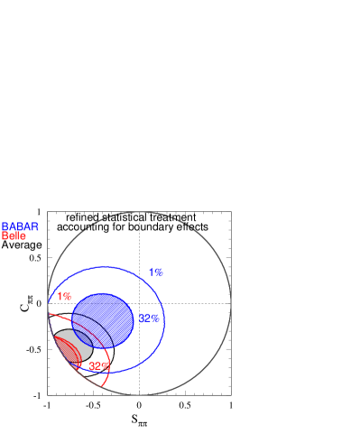
Figure 1: Confidence level at 32%percent3232\% and 1%percent11\% corresponding to BABAR and Belle results, and their average. The calculation takes into account the fact that the theoretical values are in the physical domain Sππ2+Cππ21superscriptsubscript𝑆𝜋𝜋2superscriptsubscript𝐶𝜋𝜋21S_{\pi\pi}^{2}+C_{\pi\pi}^{2}\leq 1. The ellipse located inside the shaded areas indicate the 32%percent3232\% bound obtained with the usual treatment.

If Sππexpsuperscriptsubscript𝑆𝜋𝜋expS_{\pi\pi}^{\rm exp} and Cππexpsuperscriptsubscript𝐶𝜋𝜋expC_{\pi\pi}^{\rm exp} are inside the physical domain then χ2(exp|best)=0superscript𝜒2conditionalexpbest0\chi^{2}({\rm exp}|{\rm best})=0. Whatever Sππexpsuperscriptsubscript𝑆𝜋𝜋expS_{\pi\pi}^{\rm exp} and Cππexpsuperscriptsubscript𝐶𝜋𝜋expC_{\pi\pi}^{\rm exp} are, by construction, there is a point in the physical domain where w=0𝑤0w=0: this point is {Sππbest\{S_{\pi\pi}^{\rm best},Cππbest}C_{\pi\pi}^{\rm best}\}. It is on the boundary of the physical domain if the measured values are outside 111The precise location of this point is not at the intersection of the unity-radius circle and the line joigning the measured point and the origin, but not far..

For each point {Sππhyp\{S_{\pi\pi}^{\rm hyp},Cππhyp}C_{\pi\pi}^{\rm hyp}\}, one computes w𝑤w from the values of the measurement at hand. Then, one proceeds to a (large) toy Monte-Carlo simulation to compute the probability to get a w𝑤w value larger than the one above. In principle, one should first obtain the pdf 𝒫(Sππexp,CππexpSππhyp,Cππhyp)𝒫superscriptsubscript𝑆𝜋𝜋expconditionalsuperscriptsubscript𝐶𝜋𝜋expsuperscriptsubscript𝑆𝜋𝜋hypsuperscriptsubscript𝐶𝜋𝜋hyp{\cal P}(S_{\pi\pi}^{\rm exp},C_{\pi\pi}^{\rm exp}\mid S_{\pi\pi}^{\rm hyp},C_{\pi\pi}^{\rm hyp}), which shape slightly depends on {Sππhypsuperscriptsubscript𝑆𝜋𝜋hypS_{\pi\pi}^{\rm hyp},Cππhypsuperscriptsubscript𝐶𝜋𝜋hypC_{\pi\pi}^{\rm hyp}}, and Belle does that. In practice, a mere Gaussian approximation is used, which is fair enough for the present discussion. Applying this treatment which accounts for boundary effects, one gets the contours of Fig. 1 where are drawn the CL computed from BABAR results (blue), Belle results (red) and from their average. For each of the three above sets of values, three contours are shown: the 32% (shaded area) and 1% CL ellipses provided by the treatment, and the 32% CL (smaller) ellipse obtained with the standard treatment.

BABAR results are still compatible with no-CP violation, but viewed from Belle or W.A. ones, the hypothesis of no-CP violation is excluded at a very high level.

3 Isospin Constraints on Bππ𝐵𝜋𝜋B\rightarrow\pi\pi

The constraints implied by SU(2) on the Bππ𝐵𝜋𝜋B\rightarrow\pi\pi decays [1] can be expressed as:

𝒜+superscript𝒜absent\displaystyle{\cal A}^{+-} =\displaystyle= μa𝜇𝑎\displaystyle\mu a\ (2)
𝒜¯+superscript¯𝒜absent\displaystyle\overline{{\cal A}}^{+-} =\displaystyle= μa¯e+2iαeff𝜇¯𝑎superscript𝑒2𝑖subscript𝛼eff\displaystyle\mu\bar{a}\ e^{+2i\alpha_{\rm eff}} (3)
𝒜+0superscript𝒜0\displaystyle{\cal A}^{+0} =\displaystyle= μei(δα0)𝜇superscript𝑒𝑖𝛿subscript𝛼0\displaystyle\mu\ e^{i(\delta-\alpha_{0})} (4)
𝒜0superscript𝒜0\displaystyle{\cal A}^{-0} =\displaystyle= μei(δ+α0)𝜇superscript𝑒𝑖𝛿subscript𝛼0\displaystyle\mu\ e^{i(\delta+\alpha_{0})} (5)
𝒜00superscript𝒜00\displaystyle{\cal A}^{00} =\displaystyle= 𝒜+0𝒜+2=μei(δα0)(1a2e+i(α0δ))superscript𝒜0superscript𝒜absent2𝜇superscript𝑒𝑖𝛿subscript𝛼01𝑎2superscript𝑒𝑖subscript𝛼0𝛿\displaystyle{\cal A}^{+0}-{{\cal A}^{+-}\over\sqrt{2}}=\mu\ e^{i(\delta-\alpha_{0})}\left(1-{a\over\sqrt{2}}\ e^{+i(\alpha_{0}-\delta)}\right) (6)
𝒜¯00superscript¯𝒜00\displaystyle\overline{{\cal A}}^{00} =\displaystyle= 𝒜0𝒜¯+2=μei(δ+α0)(1a¯2ei(α0+δ2αeff)),superscript𝒜0superscript¯𝒜absent2𝜇superscript𝑒𝑖𝛿subscript𝛼01¯𝑎2superscript𝑒𝑖subscript𝛼0𝛿2subscript𝛼eff\displaystyle{\cal A}^{-0}-{\overline{{\cal A}}^{+-}\over\sqrt{2}}=\mu\ e^{i(\delta+\alpha_{0})}\left(1-{\bar{a}\over\sqrt{2}}\ e^{-i(\alpha_{0}+\delta-2\alpha_{\rm eff})}\right)~{}, (7)

where

  • 𝒜+/𝒜¯+superscript𝒜absentsuperscript¯𝒜absent{\cal A}^{+-}/\overline{{\cal A}}^{+-} ;𝒜+0/𝒜0superscript𝒜0superscript𝒜0{\cal A}^{+0}/{\cal A}^{-0} ;𝒜00/𝒜¯00superscript𝒜00superscript¯𝒜00{\cal A}^{00}/\overline{{\cal A}}^{00} are the amplitudes of the B/B¯π+π𝐵¯𝐵superscript𝜋superscript𝜋B/\overline{B}\rightarrow\pi^{+}\pi^{-}; π+π0superscript𝜋superscript𝜋0\pi^{+}\pi^{0},ππ0superscript𝜋superscript𝜋0\pi^{-}\pi^{0}; π0π0superscript𝜋0superscript𝜋0\pi^{0}\pi^{0} decays, respectively,

  • μ𝜇\mu, a𝑎a and a¯¯𝑎\bar{a} are three unknown real (and positive) parameters which drive the strenght of the branching ratios,

  • α0subscript𝛼0\alpha_{0}, αeffsubscript𝛼eff\alpha_{\rm eff} and δ𝛿\delta are three phases (α0subscript𝛼0\alpha_{0} is the true value of the angle α𝛼\alpha),

  • the phase convention chosen here is such that 𝒜+superscript𝒜absent{\cal A}^{+-} is real positive.

Although αeffsubscript𝛼eff\alpha_{\rm eff} bears information on CP violation, its value is technically independent of the α0subscript𝛼0\alpha_{0} value: the presence of Penguins diagrams breaks down the relationship, if they are theoretically unknown, which is assumed here. In terms of the above six unknown parameters, the six physical observables take the form 222To take into account the fact that the lifetime of charged and neutral B𝐵B are different, every branching ratio should be divided by the corresponding lifetime: +superscriptabsent{\cal B}^{+-}, +0superscript0{\cal B}^{+0} and 00superscript00{\cal B}^{00} become then respectively +τB0superscriptabsent𝜏superscript𝐵0\frac{{\cal B}^{+-}}{\tau{B^{0}}}, +0τB+superscript0𝜏superscript𝐵\frac{{\cal B}^{+0}}{\tau{B^{+}}} and 00τB0superscript00𝜏superscript𝐵0\frac{{\cal B}^{00}}{\tau{B^{0}}}. All numerical results are obtained with this modification, but for the sake of clarity the lifetimes do not appear explicitly in the formulae. The values used for the lifetimes are taken from [15].:

+superscriptabsent\displaystyle{\cal B}^{+-} =\displaystyle= 12(𝒜+2+𝒜¯+2)=μ212(a2+a¯2)12superscriptdelimited-∣∣superscript𝒜absent2superscriptdelimited-∣∣superscript¯𝒜absent2superscript𝜇212superscript𝑎2superscript¯𝑎2\displaystyle{1\over 2}(\mid{\cal A}^{+-}\mid^{2}+\mid\overline{{\cal A}}^{+-}\mid^{2})=\mu^{2}{1\over 2}(a^{2}+\bar{a}^{2}) (8)
+0superscript0\displaystyle{\cal B}^{+0} =\displaystyle= μ2superscript𝜇2\displaystyle\mu^{2} (9)
00superscript00\displaystyle{\cal B}^{00} =\displaystyle= 12(𝒜002+𝒜¯002)=μ212(2+12(a2+a¯2)2(ac+a¯c¯))12superscriptdelimited-∣∣superscript𝒜002superscriptdelimited-∣∣superscript¯𝒜002superscript𝜇212212superscript𝑎2superscript¯𝑎22𝑎𝑐¯𝑎¯𝑐\displaystyle{1\over 2}(\mid{\cal A}^{00}\mid^{2}+\mid\overline{{\cal A}}^{00}\mid^{2})=\mu^{2}{1\over 2}\left(2+{1\over 2}(a^{2}+\bar{a}^{2})-\sqrt{2}(ac+\bar{a}\bar{c})\right) (10)
Cππsubscript𝐶𝜋𝜋\displaystyle C_{\pi\pi} =\displaystyle= 𝒜+2𝒜¯+2𝒜+2+𝒜¯+2=a2a¯2a2+a¯2superscriptdelimited-∣∣superscript𝒜absent2superscriptdelimited-∣∣superscript¯𝒜absent2superscriptdelimited-∣∣superscript𝒜absent2superscriptdelimited-∣∣superscript¯𝒜absent2superscript𝑎2superscript¯𝑎2superscript𝑎2superscript¯𝑎2\displaystyle{\mid{\cal A}^{+-}\mid^{2}-\mid\overline{{\cal A}}^{+-}\mid^{2}\over\mid{\cal A}^{+-}\mid^{2}+\mid\overline{{\cal A}}^{+-}\mid^{2}}={a^{2}-\bar{a}^{2}\over a^{2}+\bar{a}^{2}} (11)
Sππsubscript𝑆𝜋𝜋\displaystyle S_{\pi\pi} =\displaystyle= 2Im(𝒜+𝒜¯+)𝒜+2+𝒜¯+2=2aa¯a2+a¯2sin(2αeff)=1Cππ2sin(2αeff)2Imsuperscript𝒜absentsuperscriptsuperscript¯𝒜absentsuperscriptdelimited-∣∣superscript𝒜absent2superscriptdelimited-∣∣superscript¯𝒜absent22𝑎¯𝑎superscript𝑎2superscript¯𝑎22subscript𝛼eff1superscriptsubscript𝐶𝜋𝜋22subscript𝛼eff\displaystyle{-2{\rm Im}({\cal A}^{+-}{\overline{{\cal A}}^{+-}}^{\ast})\over\mid{\cal A}^{+-}\mid^{2}+\mid\overline{{\cal A}}^{+-}\mid^{2}}={2a\bar{a}\over a^{2}+\bar{a}^{2}}\sin(2\alpha_{\rm eff})=\sqrt{1-C_{\pi\pi}^{2}}\sin(2\alpha_{\rm eff}) (12)
C00subscript𝐶00\displaystyle C_{00} =\displaystyle= 𝒜002𝒜¯002𝒜002+𝒜¯002=12(a2a¯2)2(aca¯c¯)2+12(a2+a¯2)2(ac+a¯c¯)superscriptdelimited-∣∣superscript𝒜002superscriptdelimited-∣∣superscript¯𝒜002superscriptdelimited-∣∣superscript𝒜002superscriptdelimited-∣∣superscript¯𝒜00212superscript𝑎2superscript¯𝑎22𝑎𝑐¯𝑎¯𝑐212superscript𝑎2superscript¯𝑎22𝑎𝑐¯𝑎¯𝑐\displaystyle{\mid{\cal A}^{00}\mid^{2}-\mid\overline{{\cal A}}^{00}\mid^{2}\over\mid{\cal A}^{00}\mid^{2}+\mid\overline{{\cal A}}^{00}\mid^{2}}={{1\over 2}(a^{2}-\bar{a}^{2})-\sqrt{2}(ac-\bar{a}\bar{c})\over 2+{1\over 2}(a^{2}+\bar{a}^{2})-\sqrt{2}(ac+\bar{a}\bar{c})} (13)

where it proves convenient to use the two quantities c𝑐c and c¯¯𝑐\bar{c} defined as:

c𝑐\displaystyle c =\displaystyle= cos(ϕ),ϕ=α0δitalic-ϕitalic-ϕsubscript𝛼0𝛿\displaystyle\cos(\phi),~{}~{}~{}~{}\phi~{}=~{}\alpha_{0}-\delta (14)
c¯¯𝑐\displaystyle\bar{c} =\displaystyle= cos(ϕ¯),ϕ¯=α0+δ2αeff.¯italic-ϕ¯italic-ϕsubscript𝛼0𝛿2subscript𝛼eff\displaystyle\cos(\overline{\phi}),~{}~{}~{}~{}\overline{\phi}~{}=~{}\alpha_{0}+\delta-2\alpha_{\rm eff}~{}. (15)

The quantity S00subscript𝑆00S_{00}, the analogous for π0π0superscript𝜋0superscript𝜋0\pi^{0}\pi^{0} of Sππsubscript𝑆𝜋𝜋S_{\pi\pi}, could also be considered. Its expression is :

S00=2sin(2α0)+aa¯sin(2αeff)a2sin(α0+δ)a¯2sin(α0δ+2αeff)2+12(a2+a¯2)2(ac+a¯c¯).subscript𝑆0022subscript𝛼0𝑎¯𝑎2subscript𝛼eff𝑎2subscript𝛼0𝛿¯𝑎2subscript𝛼0𝛿2subscript𝛼eff212superscript𝑎2superscript¯𝑎22𝑎𝑐¯𝑎¯𝑐S_{00}={2\sin(2\alpha_{0})+{a\bar{a}}\sin(2\alpha_{\rm eff})-{a\sqrt{2}}\sin(\alpha_{0}+\delta)-{\bar{a}\sqrt{2}}\sin(\alpha_{0}-\delta+2\alpha_{\rm eff})\over 2+{1\over 2}(a^{2}+\bar{a}^{2})-\sqrt{2}(ac+\bar{a}\bar{c})}~{}. (16)

However, its measurement (through Dalitz decays of at least one of the π0superscript𝜋0{\pi^{0}}) implies huge statistics and it is assumed that S00subscript𝑆00S_{00} is not measurable. The six remaining measurements +superscriptabsent{\cal B}^{+-}, +0superscript0{\cal B}^{+0}, 00superscript00{\cal B}^{00}, Sππsubscript𝑆𝜋𝜋S_{\pi\pi}, Cππsubscript𝐶𝜋𝜋C_{\pi\pi} and C00subscript𝐶00C_{00} can in principle fix the six unknowns, including α𝛼\alpha, at least up to multiple solutions. The phases αeffsubscript𝛼eff\alpha_{\rm eff}, δ𝛿\delta and α0subscript𝛼0\alpha_{0} enter the above six Eqs.(8-13) only through c𝑐c, c¯¯𝑐\bar{c} and sin(2αeff)2subscript𝛼eff\sin(2\alpha_{\rm eff}), which are invariant through the three changes ϕϕitalic-ϕitalic-ϕ\phi\leftrightarrow-\phi, ϕ¯ϕ¯¯italic-ϕ¯italic-ϕ\overline{\phi}\leftrightarrow-\overline{\phi} and 2αeffπ2αeff2subscript𝛼eff𝜋2subscript𝛼eff2\alpha_{\rm eff}\leftrightarrow\pi-2\alpha_{\rm eff}. Hence, there are 8 mirror solutions in the range [0,π]0𝜋[0,\pi] (16 in the full range [0,2π]02𝜋[0,2\pi]). These 8 mirror solutions are explicited in Table 2 (up to a ±πplus-or-minus𝜋\pm\pi shift to bring them back in the range [0,π]0𝜋[0,\pi]) where the first row indicates the true solution for the triplet (α𝛼\alpha,δ𝛿\delta,αeffsubscript𝛼eff\alpha_{\rm eff}).

Solutions α𝛼\alpha δ𝛿\delta αeffsubscript𝛼eff\alpha_{\rm eff} ϕitalic-ϕ\phi ϕ¯¯italic-ϕ\overline{\phi}
1 α0subscript𝛼0\alpha_{0} δ𝛿\delta αeffsubscript𝛼eff\alpha_{\rm eff} ϕitalic-ϕ\phi ϕ¯¯italic-ϕ\overline{\phi}
2 δ𝛿\delta α0subscript𝛼0\alpha_{0} αeffsubscript𝛼eff\alpha_{\rm eff} ϕitalic-ϕ-\phi ϕ¯¯italic-ϕ\overline{\phi}
3 α0+2αeffsubscript𝛼02subscript𝛼eff-\alpha_{0}+2\alpha_{\rm eff} δ+2αeff𝛿2subscript𝛼eff-\delta+2\alpha_{\rm eff} αeffsubscript𝛼eff\alpha_{\rm eff} ϕitalic-ϕ-\phi ϕ¯¯italic-ϕ-\overline{\phi}
4 δ+2αeff𝛿2subscript𝛼eff-\delta+2\alpha_{\rm eff} α0+2αeffsubscript𝛼02subscript𝛼eff-\alpha_{0}+2\alpha_{\rm eff} αeffsubscript𝛼eff\alpha_{\rm eff} ϕitalic-ϕ\phi ϕ¯¯italic-ϕ-\overline{\phi}
5 π2α0𝜋2subscript𝛼0{\pi\over 2}-\alpha_{0} π2δ𝜋2𝛿{\pi\over 2}-\delta π2αeff𝜋2subscript𝛼eff{\pi\over 2}-\alpha_{\rm eff} ϕitalic-ϕ-\phi ϕ¯¯italic-ϕ-\overline{\phi}
6 π2δ𝜋2𝛿{\pi\over 2}-\delta π2α0𝜋2subscript𝛼0{\pi\over 2}-\alpha_{0} π2αeff𝜋2subscript𝛼eff{\pi\over 2}-\alpha_{\rm eff} ϕitalic-ϕ\phi ϕ¯¯italic-ϕ-\overline{\phi}
7 π2+α02αeff𝜋2subscript𝛼02subscript𝛼eff{\pi\over 2}+\alpha_{0}-2\alpha_{\rm eff} π2+δ2αeff𝜋2𝛿2subscript𝛼eff{\pi\over 2}+\delta-2\alpha_{\rm eff} π2αeff𝜋2subscript𝛼eff{\pi\over 2}-\alpha_{\rm eff} ϕitalic-ϕ\phi ϕ¯¯italic-ϕ\overline{\phi}
8 π2+δ2αeff𝜋2𝛿2subscript𝛼eff{\pi\over 2}+\delta-2\alpha_{\rm eff} π2+α02αeff𝜋2subscript𝛼02subscript𝛼eff{\pi\over 2}+\alpha_{0}-2\alpha_{\rm eff} π2αeff𝜋2subscript𝛼eff{\pi\over 2}-\alpha_{\rm eff} ϕitalic-ϕ-\phi ϕ¯¯italic-ϕ\overline{\phi}
Table 2: Mirror solutions for α𝛼\alpha in the range [0,π]0𝜋[0,\pi]. All the 8 triplets (α,δ,αeff𝛼𝛿subscript𝛼eff\alpha,\delta,\alpha_{\rm eff}) yield the same values for c𝑐c, c¯¯𝑐\bar{c} and sin(2αeff)2subscript𝛼eff\sin(2\alpha_{\rm eff}). Solutions (5) to (8) are just π/2𝜋2\pi/2 minus solutions (1) to (4). The 8 mirror solutions are strictly equivallent. They cannot be distinguished if no input is added to the ones of Eqs.(8-13), like S00subscript𝑆00S_{00} for example.

It is worth remarking that the mirror solutions appear in pairs symmetrical around αeffsubscript𝛼eff\alpha_{\rm eff}:

α(1)αeff𝛼1subscript𝛼eff\displaystyle\alpha(1)-\alpha_{\rm eff} =\displaystyle= αeffα(3)subscript𝛼eff𝛼3\displaystyle\alpha_{\rm eff}-\alpha(3) (17)
α(2)αeff𝛼2subscript𝛼eff\displaystyle\alpha(2)-\alpha_{\rm eff} =\displaystyle= αeffα(4)subscript𝛼eff𝛼4\displaystyle\alpha_{\rm eff}-\alpha(4) (18)

and that, if the mirror solutions closest to the true value α0subscript𝛼0\alpha_{0} are solutions (2)-(3)-(4), denoting them α(ii,iii,iv)𝛼𝑖𝑖𝑖𝑖𝑖𝑖𝑣\alpha(ii,iii,iv) according to their closeness rank:

α(ii)α0α(iii)α0α(iv)α0.delimited-∣∣𝛼𝑖𝑖subscript𝛼0delimited-∣∣𝛼𝑖𝑖𝑖subscript𝛼0delimited-∣∣𝛼𝑖𝑣subscript𝛼0\mid\alpha(ii)-\alpha_{0}\mid\leq\mid\alpha(iii)-\alpha_{0}\mid\leq\mid\alpha(iv)-\alpha_{0}\mid~{}. (19)

It follows, from Table 2, that the fourth-rank mirror solution cannot be too close, nor too far away from α0α(i)subscript𝛼0𝛼𝑖\alpha_{0}\equiv\alpha(i), since it satisfies the double inequality:

2α(ii)α0α(iv)α02α(iii)α0.2delimited-∣∣𝛼𝑖𝑖subscript𝛼0delimited-∣∣𝛼𝑖𝑣subscript𝛼02delimited-∣∣𝛼𝑖𝑖𝑖subscript𝛼02\mid\alpha(ii)-\alpha_{0}\mid\leq\mid\alpha(iv)-\alpha_{0}\mid\leq 2\mid\alpha(iii)-\alpha_{0}\mid~{}. (20)

Therefore, if the second-rank mirror solution α(ii)𝛼𝑖𝑖\alpha(ii) is near α0subscript𝛼0\alpha_{0}, while the third-rank mirror solution α(iii)𝛼𝑖𝑖𝑖\alpha(iii) is also creeping close, then the fourth-rank solution α(iv)𝛼𝑖𝑣\alpha(iv) is nor far either: in that case, α0subscript𝛼0\alpha_{0} will not be precisely measured. This topic is discussed in Section 4.4 in the light of the Grossman-Quinn bound.

4 Algebra

In this section one deals with some stark mathematics. The algebra involved being quite simple, only the results are presented: they are important for the next sections. It is demonstrated in passing that the sign of cos(2αeff)2subscript𝛼eff\cos(2\alpha_{\rm eff}) is firmly established by BABAR data, and the current CKM fit results. Below, are discussed the two types of bounds one may find in the literature: lower (and upper) bounds on 00superscript00{\cal B}^{00}, and upper bounds on ααeffdelimited-∣∣𝛼subscript𝛼eff\mid\alpha-\alpha_{\rm eff}\mid. These bounds are of some interest, but they can also be misleading. Furthermore, because of the limited precision on the measurements they use, all bounds (and the new bound of Eq.(24) is no exception) do not provide more than qualitative insights. To turn a bound value into a quantitative statement, one should append the CL it refers to, and this implies to have recourse to fits, which is done in Section 5.

4.1 New bounds on 00superscript00{\cal B}^{00}

New bounds on 00superscript00{\cal B}^{00} are presented, using the current knowledge on α𝛼\alpha. The value determined by the standard CKM fit is 96±13oplus-or-minus96superscript13𝑜96\pm 13^{o} (1.67±0.23radplus-or-minus1.670.23rad1.67\pm 0.23~{}\rm rad[16]. Using α𝛼\alpha presents several interests:

  • to help cornering 00superscript00{\cal B}^{00}. For the time being, the question is not yet to pinpoint α𝛼\alpha thanks to Bππ𝐵𝜋𝜋B\rightarrow\pi\pi decays, but to evaluate the chances one has to do so in the close or distant future. With that respect, one is longing for a robust estimate of 00superscript00{\cal B}^{00}, and every tools at hand should be used to secure it. The information on α𝛼\alpha must be used to this end as well,

  • to derive the sign of cos(2αeff)2subscript𝛼eff\cos(2\alpha_{\rm eff}) (Section 4.1.2),

  • to understand the behavior of the mirror solutions (Section 5.1).

Assuming that α𝛼\alpha is known, the set of equations for the Bππ𝐵𝜋𝜋B\rightarrow\pi\pi amplitudes implies the following lower bounds for the B0π0π0superscript𝐵0superscript𝜋0superscript𝜋0B^{0}\rightarrow\pi^{0}\pi^{0} branching ratio 333They are obtained by deriving 00superscript00{\cal B}^{00} with respect to δ𝛿\delta.:

α:l±00subscriptsuperscript00:𝛼limit-fromlplus-or-minus\displaystyle{\cal B}^{00}_{\alpha:{\rm l}\pm} =\displaystyle= +0+12++0+(1+O±)superscript012superscriptabsentsuperscript0superscriptabsent1subscript𝑂plus-or-minus\displaystyle{\cal B}^{+0}+{1\over 2}{\cal B}^{+-}-\sqrt{{\cal B}^{+0}{\cal B}^{+-}(1+O_{\pm})} (21)
O±subscript𝑂plus-or-minus\displaystyle O_{\pm} =\displaystyle= 1Cππ2cos(2(α0αeff))1superscriptsubscript𝐶𝜋𝜋22subscript𝛼0subscript𝛼eff\displaystyle\sqrt{1-C_{\pi\pi}^{2}}\ \cos(2(\alpha_{0}-\alpha_{\rm eff})) (22)
=\displaystyle= ±(1sin2(2α0))(1Cππ2Sππ2)+sin(2α0)Sππplus-or-minus1superscript22subscript𝛼01superscriptsubscript𝐶𝜋𝜋2superscriptsubscript𝑆𝜋𝜋22subscript𝛼0subscript𝑆𝜋𝜋\displaystyle\pm\sqrt{(1-\sin^{2}(2\alpha_{0}))(1-C_{\pi\pi}^{2}-S_{\pi\pi}^{2})}+\sin(2\alpha_{0})S_{\pi\pi} (23)

where ±plus-or-minus\pm in O±subscript𝑂plus-or-minusO_{\pm} is the sign of the product cos(2αeff)cos(2α0)2subscript𝛼eff2subscript𝛼0\cos(2\alpha_{\rm eff})\cos(2\alpha_{0}).

They come with the upper bounds α:u±00subscriptsuperscript00:𝛼limit-fromuplus-or-minus{\cal B}^{00}_{\alpha:{\rm u}\pm} obtained by reversing the sign in front of the square root. However, the upper bounds are not very relevant, being much weaker than the direct experimental upper limit.

4.1.1 The reBound

The bound α:l+00subscriptsuperscript00:𝛼limit-froml{\cal B}^{00}_{\alpha:{\rm l}+} obtained when cos(2αeff)cos(2α0)2subscript𝛼eff2subscript𝛼0\cos(2\alpha_{\rm eff})\cos(2\alpha_{0}) is taken to be positive is referred to as the reBound:

α:l+00=+0+12++0+(1+O+)subscriptsuperscript00:𝛼limit-fromlsuperscript012superscriptabsentsuperscript0superscriptabsent1subscript𝑂{\cal B}^{00}_{\alpha:{\rm l}+}={\cal B}^{+0}+{1\over 2}{\cal B}^{+-}-\sqrt{{\cal B}^{+0}{\cal B}^{+-}(1+O_{+})} (24) O+=(1sin2(2α0))(1Cππ2Sππ2)+sin(2α0)Sππsubscript𝑂1superscript22subscript𝛼01superscriptsubscript𝐶𝜋𝜋2superscriptsubscript𝑆𝜋𝜋22subscript𝛼0subscript𝑆𝜋𝜋O_{+}=\sqrt{(1-\sin^{2}(2\alpha_{0}))(1-C_{\pi\pi}^{2}-S_{\pi\pi}^{2})}+\sin(2\alpha_{0})S_{\pi\pi} (25)

The alternative bound α:l00subscriptsuperscript00:𝛼limit-froml{\cal B}^{00}_{\alpha:{\rm l}-} is considered in the next section.

The reBound can be compared with previous bounds [17, 18], the strongest lower one being the Gronau-London-Sinha-Sinha (GLSS) bound [19]:

GLSS:l00=+0+12++0+(1+1Cππ2)subscriptsuperscript00:GLSSlsuperscript012superscriptabsentsuperscript0superscriptabsent11superscriptsubscript𝐶𝜋𝜋2{\cal B}^{00}_{\rm GLSS:l}={\cal B}^{+0}+{1\over 2}{\cal B}^{+-}-\sqrt{{\cal B}^{+0}{\cal B}^{+-}\left(1+\sqrt{1-C_{\pi\pi}^{2}}\right)} (26)

which minimal value with respect to Cππsubscript𝐶𝜋𝜋C_{\pi\pi} is attained for Cππ=0subscript𝐶𝜋𝜋0C_{\pi\pi}=0:

GLSS:l00[min]=+0(1+2+0)2.subscriptsuperscript00:GLSSldelimited-[]minsuperscript0superscript1superscriptabsent2superscript02{\cal B}^{00}_{\rm GLSS:l}[\rm min]={\cal B}^{+0}\left(1-\sqrt{{\cal B}^{+-}\over 2{\cal B}^{+0}}\right)^{2}~{}. (27)

It comes in pair with the upper bound GLSS:u00subscriptsuperscript00:GLSSu{\cal B}^{00}_{\rm GLSS:u} obtained by reverting the sign in front of the square root. However, as obvious from Eq.(22) the reBound is more stringent than the GLSS bound, which it reproduces if no knowledge on α𝛼\alpha is assumed. The largest difference is obtained with the Belle measurements (Cππ2+Sππ2=1superscriptsubscript𝐶𝜋𝜋2superscriptsubscript𝑆𝜋𝜋21C_{\pi\pi}^{2}+S_{\pi\pi}^{2}=1), which, taken together with the value α0=90osubscript𝛼0superscript90𝑜\alpha_{0}~{}=~{}90^{o}, imply the new lower limit 00>2.3superscript002.3{\cal B}^{00}>2.3, while the weaker bound of Eq.(26) is 00>0.7superscript000.7{\cal B}^{00}>0.7 (see Table 3).

Using unadorned standard error propagation to estimate the precision of the bound, one gets for the reBound, α=96o𝛼superscript96𝑜\alpha~{}=~{}96^{o}, and,

BABAR values:

α:l+00=0.60.3+0.5[+0]0.1+0.2[+]0.0+0.1[Sππ]0.0+0.1[Cππ]0.0+0.2[α]subscriptsuperscript00:𝛼limit-fromlsubscriptsuperscript0.60.50.3subscriptsuperscriptdelimited-[]superscript00.20.1subscriptsuperscriptdelimited-[]superscriptabsent0.10.0subscriptsuperscriptdelimited-[]subscript𝑆𝜋𝜋0.10.0subscriptsuperscriptdelimited-[]subscript𝐶𝜋𝜋0.20.0delimited-[]𝛼{\cal B}^{00}_{\alpha:{\rm l}+}=0.6^{+0.5}_{-0.3}[{\cal B}^{+0}]^{+0.2}_{-0.1}[{\cal B}^{+-}]^{+0.1}_{-0.0}[S_{\pi\pi}]^{+0.1}_{-0.0}[C_{\pi\pi}]^{+0.2}_{-0.0}[\alpha] (28)

Belle values:

α:l+00=1.90.5+0.7[+0]0.0+0.1[+]0.1+0.1[Sππ]0.0+0.0[Cππ]0.4+0.6[α]subscriptsuperscript00:𝛼limit-fromlsubscriptsuperscript1.90.70.5subscriptsuperscriptdelimited-[]superscript00.10.0subscriptsuperscriptdelimited-[]superscriptabsent0.10.1subscriptsuperscriptdelimited-[]subscript𝑆𝜋𝜋0.00.0subscriptsuperscriptdelimited-[]subscript𝐶𝜋𝜋0.60.4delimited-[]𝛼{\cal B}^{00}_{\alpha:{\rm l}+}=1.9^{+0.7}_{-0.5}[{\cal B}^{+0}]^{+0.1}_{-0.0}[{\cal B}^{+-}]^{+0.1}_{-0.1}[S_{\pi\pi}]^{+0.0}_{-0.0}[C_{\pi\pi}]^{+0.6}_{-0.4}[\alpha] (29)

and world average values:

α:l+00=1.10.3+0.3[+0]0.1+0.1[+]0.2+0.0[Sππ]0.1+0.2[Cππ]0.2+0.4[α]subscriptsuperscript00:𝛼limit-fromlsubscriptsuperscript1.10.30.3subscriptsuperscriptdelimited-[]superscript00.10.1subscriptsuperscriptdelimited-[]superscriptabsent0.00.2subscriptsuperscriptdelimited-[]subscript𝑆𝜋𝜋0.20.1subscriptsuperscriptdelimited-[]subscript𝐶𝜋𝜋0.40.2delimited-[]𝛼{\cal B}^{00}_{\alpha:{\rm l}+}=1.1^{+0.3}_{-0.3}[{\cal B}^{+0}]^{+0.1}_{-0.1}[{\cal B}^{+-}]^{+0.0}_{-0.2}[S_{\pi\pi}]^{+0.2}_{-0.1}[C_{\pi\pi}]^{+0.4}_{-0.2}[\alpha] (30)

where the source of the uncertainty on the bound is specified within brackets. Whereas this tells that the main negative inaccuracy on the reBound value stems from the branching ratio +0superscript0{\cal B}^{+0}, one cannot infer much else: the errors are large and correlated, hence they cannot be added in quadrature. Anyway, one should keep in mind that the actual 90% CL lower limit on 00superscript00{\cal B}^{00} can hardly be guessed from back of the envelope calculations.

The numerical results for the reBound for BABAR, Belle and world average are summarized in Table 3 for three different α0subscript𝛼0\alpha_{0} values. In this table are also given numerical values of other bounds presented in the following sections.

Bounds GLSS:l00subscriptsuperscript00:GLSSl{\cal B}^{00}_{\rm GLSS:l} α:l+00subscriptsuperscript00:𝛼limit-froml{\cal B}^{00}_{\alpha:{\rm l}+}: reBound α:l00subscriptsuperscript00:𝛼limit-froml{\cal B}^{00}_{\alpha:{\rm l}-}: tough Bound 00/+0superscript00superscript0{\cal B}^{00}/{\cal B}^{+0} SGQsubscript𝑆GQS_{\rm GQ}
α𝛼\alpha 90osuperscript90𝑜90^{o} 96osuperscript96𝑜96^{o} 110osuperscript110𝑜110^{o} 90osuperscript90𝑜90^{o} 96osuperscript96𝑜96^{o} 110osuperscript110𝑜110^{o}
BABAR 0.60.60.6 0.70.70.7 0.60.60.6 0.60.60.6 5.95.95.9 5.25.25.2 3.83.83.8 0.40.40.4 0.40.40.4
Belle 0.70.70.7 2.32.32.3 1.91.91.9 1.21.21.2 2.32.32.3 1.91.91.9 1.21.21.2 0.40.40.4 0.30.30.3
W.A. 0.70.70.7 1.31.31.3 1.11.11.1 0.70.70.7 3.83.83.8 3.33.33.3 2.22.22.2 0.40.40.4 0.40.40.4
Table 3: Numerical values for the different bounds: the GLSS bound, the reBound, the tough Bound, the original (approximate) Grossman-Quinn bound and the exact Grossman-Quinn bound. Branching ratios are quoted in the 106superscript10610^{-6} unit. The last two values are discussed in Section 4.4.

4.1.2 The tough Bound

The hypothesis that the sign of cos(2αeff)2subscript𝛼eff\cos(2\alpha_{\rm eff}) is opposite to the sign of cos(2α0)2subscript𝛼0\cos(2\alpha_{0}) is now made. A more stringent bound is then obtained:

α:l00=+0+12++0+(1+O)subscriptsuperscript00:𝛼limit-fromlsuperscript012superscriptabsentsuperscript0superscriptabsent1subscript𝑂{\cal B}^{00}_{\alpha:{\rm l}-}={\cal B}^{+0}+{1\over 2}{\cal B}^{+-}-\sqrt{{\cal B}^{+0}{\cal B}^{+-}(1+O_{-})} (31)

which is referred to as the tough Bound. For Belle, since Cππ2+Sππ2=1superscriptsubscript𝐶𝜋𝜋2superscriptsubscript𝑆𝜋𝜋21C_{\pi\pi}^{2}+S_{\pi\pi}^{2}=1, the tough Bound is identical to the reBound. However, for BABAR and for the world average, reverting the sign makes a huge difference. The precision on the tough Bound for α=96o𝛼superscript96𝑜\alpha~{}=~{}96^{o} is, for the BABAR values:

α:l00=5.20.9+1.0[+0]0.2+0.2[+]0.5+0.5[Sππ]0.2+0.1[Cππ]0.9+0.9[α]subscriptsuperscript00:𝛼limit-fromlsubscriptsuperscript5.21.00.9subscriptsuperscriptdelimited-[]superscript00.20.2subscriptsuperscriptdelimited-[]superscriptabsent0.50.5subscriptsuperscriptdelimited-[]subscript𝑆𝜋𝜋0.10.2subscriptsuperscriptdelimited-[]subscript𝐶𝜋𝜋0.90.9delimited-[]𝛼{\cal B}^{00}_{\alpha:{\rm l}-}=5.2^{+1.0}_{-0.9}[{\cal B}^{+0}]^{+0.2}_{-0.2}[{\cal B}^{+-}]^{+0.5}_{-0.5}[S_{\pi\pi}]^{+0.1}_{-0.2}[C_{\pi\pi}]^{+0.9}_{-0.9}[\alpha] (32)

for Belle:

α:l00=1.90.5+0.7[+0]0.0+0.1[+]0.1+0.1[Sππ]0.0+0.0[Cππ]0.4+0.6[α]subscriptsuperscript00:𝛼limit-fromlsubscriptsuperscript1.90.70.5subscriptsuperscriptdelimited-[]superscript00.10.0subscriptsuperscriptdelimited-[]superscriptabsent0.10.1subscriptsuperscriptdelimited-[]subscript𝑆𝜋𝜋0.00.0subscriptsuperscriptdelimited-[]subscript𝐶𝜋𝜋0.60.4delimited-[]𝛼{\cal B}^{00}_{\alpha:{\rm l}-}=1.9^{+0.7}_{-0.5}[{\cal B}^{+0}]^{+0.1}_{-0.0}[{\cal B}^{+-}]^{+0.1}_{-0.1}[S_{\pi\pi}]^{+0.0}_{-0.0}[C_{\pi\pi}]^{+0.6}_{-0.4}[\alpha] (33)

and for the world average:

α:l00=3.30.4+0.5[+0]0.0+0.0[+]0.0+0.4[Sππ]0.3+0.2[Cππ]0.7+0.7[α].subscriptsuperscript00:𝛼limit-fromlsubscriptsuperscript3.30.50.4subscriptsuperscriptdelimited-[]superscript00.00.0subscriptsuperscriptdelimited-[]superscriptabsent0.40.0subscriptsuperscriptdelimited-[]subscript𝑆𝜋𝜋0.20.3subscriptsuperscriptdelimited-[]subscript𝐶𝜋𝜋0.70.7delimited-[]𝛼{\cal B}^{00}_{\alpha:{\rm l}-}=3.3^{+0.5}_{-0.4}[{\cal B}^{+0}]^{+0.0}_{-0.0}[{\cal B}^{+-}]^{+0.4}_{-0.0}[S_{\pi\pi}]^{+0.2}_{-0.3}[C_{\pi\pi}]^{+0.7}_{-0.7}[\alpha]~{}. (34)

These tough Bound values are, for BABAR and W.A., firm enough to be barely consistent with the measurement of 00superscript00{\cal B}^{00} (Table 1): the hypothesis cos(2αeff)cos(2α0)<02subscript𝛼eff2subscript𝛼00\cos(2\alpha_{\rm eff})\cos(2\alpha_{0})<0 is disfavored. On the other hand, the sign of cos(2α)2𝛼\cos(2\alpha) is well defined to be negative by the current state of the art of CKM fits. Hence, the tough Bound suggests cos(2αeff)<02subscript𝛼eff0\cos(2\alpha_{\rm eff})<0.

4.2 The C00subscript𝐶00C_{00} function

The asymmetry term C00subscript𝐶00C_{00} (Eq.(13)) has not been yet measured due to the insufficient luminosity. From the knowledge of α𝛼\alpha, once the three branching ratios +superscriptabsent{\cal B}^{+-}, +0superscript0{\cal B}^{+0}, 00superscript00{\cal B}^{00} and the two asymmetries Sππsubscript𝑆𝜋𝜋S_{\pi\pi} and Cππsubscript𝐶𝜋𝜋C_{\pi\pi} are measured, C00subscript𝐶00C_{00} can be determined, up to a fourfold ambiguity:

C00±;+superscriptsubscript𝐶00plus-or-minus\displaystyle C_{00}^{\pm;+} =\displaystyle= 100(1+O+){Cππ(+0+2O+00)\displaystyle\frac{1}{{\cal B}^{00}(1+O_{+})}\Bigg{\{}-C_{\pi\pi}\left({\cal B}^{+0}-{{\cal B}^{+-}\over 2}O_{+}-{\cal B}^{00}\right) (35) ±(00α:l±00)(α:u±0000)(1O+2Cππ2)}\displaystyle\pm\sqrt{({\cal B}^{00}-{\cal B}^{00}_{\alpha:{\rm l}{\pm}})({\cal B}^{00}_{\alpha:{\rm u}{\pm}}-{\cal B}^{00})(1-O_{+}^{2}-C_{\pi\pi}^{2})}\Bigg{\}}

One obtains the two other solutions C00±;superscriptsubscript𝐶00plus-or-minusC_{00}^{\pm;-} by using Osubscript𝑂O_{-} instead of O+subscript𝑂O_{+} in the above expression. For α0=90osubscript𝛼0superscript90𝑜\alpha_{0}~{}=~{}90^{o} some simplifications occur:

O±subscript𝑂plus-or-minus\displaystyle O_{\pm} =\displaystyle= ±1Cππ2Sππ2plus-or-minus1superscriptsubscript𝐶𝜋𝜋2superscriptsubscript𝑆𝜋𝜋2\displaystyle\pm\sqrt{1-C_{\pi\pi}^{2}-S_{\pi\pi}^{2}} (36)
C00±;±superscriptsubscript𝐶00plus-or-minusplus-or-minus\displaystyle C_{00}^{\pm;\pm} =\displaystyle= 100(1+O±){Cππ(+0+2O±00)\displaystyle\frac{1}{{\cal B}^{00}(1+O_{\pm})}\Bigg{\{}-C_{\pi\pi}\left({\cal B}^{+0}-{{\cal B}^{+-}\over 2}O_{\pm}-{\cal B}^{00}\right) (37)
±Sππ(00α:l±00)(α:u±0000)}.\displaystyle\pm S_{\pi\pi}\sqrt{({\cal B}^{00}-{\cal B}^{00}_{\alpha:{\rm l}{\pm}})({\cal B}^{00}_{\alpha:{\rm u}{\pm}}-{\cal B}^{00})}\Bigg{\}}~{}.

This multivalued function is drawn on Fig. 2, for BABAR, Belle and the world average, with α=90𝛼90\alpha~{}=~{}90, 969696 and 110osuperscript110𝑜110^{o}. The 00superscript00{\cal B}^{00} axis spans the range up to 15×10615superscript10615\times 10^{-6} despite the known experimental upper bound to allow a wide view on the C00(00)subscript𝐶00superscript00C_{00}({\cal B}^{00}) function. Each of the two closed loops corresponds to a given choice for the sign of cos(2αeff)cos(2α0)2subscript𝛼eff2subscript𝛼0\cos(2\alpha_{\rm eff})\cos(2\alpha_{0}): the plain lines correspond to O+subscript𝑂O_{+}, the dotted ones to Osubscript𝑂O_{-}. The upper and lower parts of each closed loop correspond to the ±plus-or-minus\pm sign of Eq.(35). The vertical lines indicate the upper and lower bounds of the allowed 00superscript00{\cal B}^{00} range. The outermost vertical lines correspond to the reBound lower (and upper) limit, while the inner lines correspond to the tough Bound limits.

For Belle, Cππ2+Sππ2superscriptsubscript𝐶𝜋𝜋2superscriptsubscript𝑆𝜋𝜋2C_{\pi\pi}^{2}+S_{\pi\pi}^{2} being taken equal to unity and then the reBound being equal to the tough Bound, the two closed loops are superimposed.

For BABAR and the world average, both the closed loops and their upper and lower components are widely split apart. For BABAR and the W.A., the inner part open when α𝛼\alpha becomes larger, it is the contrary for the outer curves: the larger α𝛼\alpha becomes, the closer they get from each other.

The variation of the value of α𝛼\alpha affects the C00(00)subscript𝐶00superscript00C_{00}({\cal B}^{00}) function domain for BABAR, Belle and W.A. In the experimentally allowed region (00<4×10⁶superscript004superscript106{\cal B}^{00}<4\times 10^{-6}), both negative and positive values are possible for C00subscript𝐶00C_{00}. Here again, such indications are to be taken with a grain of salt since the uncertainties on the measurements are not accounted for in the discussion (but they are in Section 6).

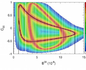
Refer to caption Refer to caption Refer to caption Refer to caption Refer to caption Refer to caption Refer to caption Refer to caption Refer to caption

Figure 2: The multivalued function C00±;±=f(+,+0,00,Sππ,Cππ,α)superscriptsubscript𝐶00plus-or-minusplus-or-minus𝑓superscriptabsentsuperscript0superscript00subscript𝑆𝜋𝜋subscript𝐶𝜋𝜋𝛼C_{00}^{\pm;\pm}=f({\cal B}^{+-},{\cal B}^{+0},{\cal B}^{00},S_{\pi\pi},C_{\pi\pi},\alpha) is drawn as a function of 00superscript00{\cal B}^{00} using α=90𝛼90\alpha~{}=~{}90 (top), 969696 (middle) as measured by the standard CKM fit, and 110osuperscript110𝑜110^{o} (bottom), for the measurements from BABAR (left), Belle (middle), and the world average (right). The outer limits correspond to cos(2αeff)cos(2α0)>02subscript𝛼eff2subscript𝛼00\cos(2\alpha_{\rm eff})\cos(2\alpha_{0})>0 (i.e. the reBound of Eq.(24)) and the inner limits to cos(2αeff)cos(2α0)<02subscript𝛼eff2subscript𝛼00\cos(2\alpha_{\rm eff})\cos(2\alpha_{0})<0 (i.e. the tough Bound of Eq.(31)).

4.3 Explicit expression for α𝛼\alpha

The identity 2α=2αeff+ϕ+ϕ¯2𝛼2subscript𝛼effitalic-ϕ¯italic-ϕ2\alpha~{}=~{}2\alpha_{\rm eff}+\phi+\overline{\phi} leads to the following expression for α𝛼\alpha:

tanα=sin(2αeff)c¯+cos(2αeff)s¯+scos(2αeff)c¯sin(2αeff)s¯+c𝛼2subscript𝛼eff¯𝑐2subscript𝛼eff¯𝑠𝑠2subscript𝛼eff¯𝑐2subscript𝛼eff¯𝑠𝑐\tan{\alpha}={\sin(2\alpha_{\rm eff})\bar{c}+\cos(2\alpha_{\rm eff})\bar{s}+s\over\cos(2\alpha_{\rm eff})\bar{c}-\sin(2\alpha_{\rm eff})\bar{s}+c} (38)

where all quantities on the right hand side can be expressed in term of the observables as follow:

sin(2αeff)2subscript𝛼eff\displaystyle\sin(2\alpha_{\rm eff}) =\displaystyle= Sππ1Cππ2subscript𝑆𝜋𝜋1superscriptsubscript𝐶𝜋𝜋2\displaystyle{S_{\pi\pi}\over\sqrt{1-C_{\pi\pi}^{2}}} (39)
cos(2αeff)2subscript𝛼eff\displaystyle\cos(2\alpha_{\rm eff}) =\displaystyle= ±1sin2(2αeff)plus-or-minus1superscript22subscript𝛼eff\displaystyle\pm\sqrt{1-\sin^{2}(2\alpha_{\rm eff})} (40)
c𝑐\displaystyle c =\displaystyle= cos(ϕ)=+0++(1+Cππ)/200(1+C00)2++0(1+Cππ)italic-ϕsuperscript0superscriptabsent1subscript𝐶𝜋𝜋2superscript001subscript𝐶002superscriptabsentsuperscript01subscript𝐶𝜋𝜋\displaystyle\cos(\phi)={{\cal B}^{+0}+{\cal B}^{+-}(1+C_{\pi\pi})/2-{\cal B}^{00}(1+C_{00})\over\sqrt{2{\cal B}^{+-}{\cal B}^{+0}(1+C_{\pi\pi})}} (41)
s𝑠\displaystyle s =\displaystyle= sin(ϕ)=±1c2italic-ϕplus-or-minus1superscript𝑐2\displaystyle\sin(\phi)=\pm\sqrt{1-c^{2}} (42)
c¯¯𝑐\displaystyle\bar{c} =\displaystyle= cos(ϕ¯)=+0++(1Cππ)/200(1C00)2++0(1Cππ)¯italic-ϕsuperscript0superscriptabsent1subscript𝐶𝜋𝜋2superscript001subscript𝐶002superscriptabsentsuperscript01subscript𝐶𝜋𝜋\displaystyle\cos(\overline{\phi})={{\cal B}^{+0}+{\cal B}^{+-}(1-C_{\pi\pi})/2-{\cal B}^{00}(1-C_{00})\over\sqrt{2{\cal B}^{+-}{\cal B}^{+0}(1-C_{\pi\pi})}} (43)
s¯¯𝑠\displaystyle\bar{s} =\displaystyle= sin(ϕ¯)=±1c¯2¯italic-ϕplus-or-minus1superscript¯𝑐2\displaystyle\sin(\overline{\phi})=\pm\sqrt{1-\bar{c}^{2}} (44)

where the eightfold ambiguity in the range [0,π]0𝜋[0,\pi] is explicited by the three arbitrary signs. One recovers the GLSS bound by requesting that both c𝑐c and c¯¯𝑐\bar{c} are smaller than one. At the edge of the allowed 00superscript00{\cal B}^{00} range, for 00=GLSS:l00superscript00subscriptsuperscript00:GLSSl{\cal B}^{00}={\cal B}^{00}_{\rm GLSS:l}, one gets:

ϕitalic-ϕ\displaystyle\phi =\displaystyle= ϕ¯=0α=αeff=δ¯italic-ϕ0𝛼subscript𝛼eff𝛿\displaystyle\overline{\phi}=0\rightarrow\alpha=\alpha_{\rm eff}=\delta (45)
C00subscript𝐶00\displaystyle C_{00} =\displaystyle= 1GLSS:l00(+2Cππ++0+(11Cππ2))1subscriptsuperscript00:GLSSlsuperscriptabsent2subscript𝐶𝜋𝜋superscript0superscriptabsent11superscriptsubscript𝐶𝜋𝜋2\displaystyle{1\over{\cal B}^{00}_{\rm GLSS:l}}\left({{\cal B}^{+-}\over 2}C_{\pi\pi}+\sqrt{{\cal B}^{+0}{\cal B}^{+-}\left(1-\sqrt{1-C_{\pi\pi}^{2}}\right)}\right) (46)
α:l+00subscriptsuperscript00:𝛼limit-froml\displaystyle{\cal B}^{00}_{\alpha:{\rm l}+} =\displaystyle= GLSS:l00.subscriptsuperscript00:GLSSl\displaystyle{\cal B}^{00}_{\rm GLSS:l}~{}. (47)

Being in an Universe where 00superscript00{\cal B}^{00} sits right at the GLSS bound may be viewed, at first glance, as good news. Indeed, in that case one has the nice equality α=αeff𝛼subscript𝛼eff\alpha~{}=~{}\alpha_{\rm eff}, as if there were no Penguins, and, as an odd bonus, one still savors direct CP violation since neither Cππsubscript𝐶𝜋𝜋C_{\pi\pi} nor C00subscript𝐶00C_{00} has to vanish. However, to be in an Universe where 00superscript00{\cal B}^{00} is simply close to the GLSS bound is bad news! Indeed, in that case, in the neighbourhood of ααeffsimilar-to-or-equals𝛼subscript𝛼eff\alpha\simeq\alpha_{\rm eff} lurk the three mirror solutions (2)-(3)-(4), while the other four solutions (5)-(6)-(7)-(8) are thrown apart. Furthermore, by construction, when one is close to the GLSS bound 00/δ=0superscript00𝛿0\partial{\cal B}^{00}/\partial\delta=0, therefore the locations of the mirror solutions (2) and (4) vary wildly with mild changes of 00superscript00{\cal B}^{00}. This subject is discussed in details in Section 5.1 and illustrated on Fig. 3. The implication that 00=GLSS:l00superscript00subscriptsuperscript00:GLSSl{\cal B}^{00}={\cal B}^{00}_{\rm GLSS:l} forces α=αeff𝛼subscript𝛼eff\alpha~{}=~{}\alpha_{\rm eff} is reminiscent of the Grossman-Quinn bound, which is discussed in the next section.

4.4 The Grossman-Quinn bound revisited

The Grossman-Quinn (GQ) bound was introduced assuming that no knowledge of α𝛼\alpha is available and C00subscript𝐶00C_{00} is not measured. It is mostly known (and used) as:

sin2(ααeff)00+0.superscript2𝛼subscript𝛼effsuperscript00superscript0\sin^{2}(\alpha-\alpha_{\rm eff})\leq{{\cal B}^{00}\over{\cal B}^{+0}}~{}. (48)

This bound appears quite peculiar owing to the results of the previous section where it was shown that α𝛼\alpha equals αeffsubscript𝛼eff\alpha_{\rm eff} if 00superscript00{\cal B}^{00} reaches the GLSS bound, not if 00superscript00{\cal B}^{00} is small. In effect, the GLSS bound is not necessarily a small number: one may thus be able to set a tight limit on the difference ααeffdelimited-∣∣𝛼subscript𝛼eff\mid\alpha-\alpha_{\rm eff}\mid even though 00superscript00{\cal B}^{00} is not small. Mathematically, the constraint on ααeffdelimited-∣∣𝛼subscript𝛼eff\mid\alpha-\alpha_{\rm eff}\mid does not stem from the size of the branching ratio, but from the proximity of the latter to its lower (or upper) bound, if no knowledge is assumed on α𝛼\alpha. Physically, there is no reason to expect ααeffsimilar-to-or-equals𝛼subscript𝛼eff\alpha\simeq\alpha_{\rm eff} except if Penguin diagrams turn out to be very small, which is not a strong hope. If it is not the case then only an unfathomable numerical accident may lead to 00GLSS:l00similar-to-or-equalssuperscript00subscriptsuperscript00:GLSSl{\cal B}^{00}\simeq{\cal B}^{00}_{\rm GLSS:l}. In fact, a straight maximization of sin2(2(ααeff))=sin2(ϕ+ϕ¯)superscript22𝛼subscript𝛼effsuperscript2italic-ϕ¯italic-ϕ\sin^{2}(2(\alpha-\alpha_{\rm eff}))=\sin^{2}(\phi+\overline{\phi}) with respect to C00subscript𝐶00C_{00} yields:

C00[max]=Cππ(+200)(+0+2+00+0++200)subscript𝐶00delimited-[]maxsubscript𝐶𝜋𝜋superscriptabsent2superscript00superscript0superscriptabsent2superscript00superscript0superscriptabsent2superscript00C_{00}[{\rm max}]=-C_{\pi\pi}\left({{\cal B}^{+-}\over 2{\cal B}^{00}}\right)\left({{\cal B}^{+0}-{{\cal B}^{+-}\over 2}+{\cal B}^{00}\over{\cal B}^{+0}+{{\cal B}^{+-}\over 2}-{\cal B}^{00}}\right) (49)

sin2(ααeff)SGQ=(00GLSS:l00)(GLSS:u0000)2++01Cππ2superscript2𝛼subscript𝛼effsubscript𝑆GQsuperscript00subscriptsuperscript00:GLSSlsubscriptsuperscript00:GLSSusuperscript002superscriptabsentsuperscript01superscriptsubscript𝐶𝜋𝜋2\sin^{2}(\alpha-\alpha_{\rm eff})~{}\leq~{}S_{\rm GQ}={\left({\cal B}^{00}-{\cal B}^{00}_{\rm GLSS:l}\right)\left({\cal B}^{00}_{\rm GLSS:u}-{\cal B}^{00}\right)\over 2{\cal B}^{+-}{\cal B}^{+0}\sqrt{1-C_{\pi\pi}^{2}}} (50)

This is not a new result: although the end product appears in a quite different form, it is derived in the same way in Ref.[19], and is approached in Ref.[18]. It is also present, albeit on a low key and in a very different looking form, in the original paper [17] itself 444Except that, in the second parenthesis, 00superscript00{\cal B}^{00} is replaced by its lower bound GLSS:l00subscriptsuperscript00:GLSSl{\cal B}^{00}_{\rm GLSS:l}, which underestimates the strength of the bound on ααeffdelimited-∣∣𝛼subscript𝛼eff\mid\alpha-\alpha_{\rm eff}\mid.. To recover the GQ bound Eq.(48) from Eq.(50), one may write:

SGQ=00+0+(11Cππ21)(00+012)(00++2+0)22+0+1Cππ2.subscript𝑆GQsuperscript00superscript011superscriptsubscript𝐶𝜋𝜋21superscript00superscript012superscriptsuperscript00superscriptabsent2superscript022superscript0superscriptabsent1superscriptsubscript𝐶𝜋𝜋2S_{\rm GQ}={{\cal B}^{00}\over{\cal B}^{+0}}+\left({1\over\sqrt{1-C_{\pi\pi}^{2}}}-1\right)\left({{\cal B}^{00}\over{\cal B}^{+0}}-{1\over 2}\right)-{\left({\cal B}^{00}+{{\cal B}^{+-}\over 2}-{\cal B}^{+0}\right)^{2}\over 2{\cal B}^{+0}{\cal B}^{+-}\sqrt{1-C_{\pi\pi}^{2}}}~{}. (51)

With BABAR, Belle and W.A. values both (competing) additionnal terms are small by chance. The second term is very small for two reasons: because (for BABAR) Cππ20.04similar-to-or-equalssuperscriptsubscript𝐶𝜋𝜋20.04C_{\pi\pi}^{2}\simeq 0.04, and because (for all) 00/+00.41/2similar-to-or-equalssuperscript00superscript00.4similar-to-or-equals12{\cal B}^{00}/{\cal B}^{+0}\simeq 0.4\simeq 1/2. The third term is small because 00superscript00{\cal B}^{00} is closed to +0+/2superscript0superscriptabsent2{\cal B}^{+0}-{\cal B}^{+-}/2.

Hence the validity of the approximation of Eq.(48), when it applies, also deprives the GQ bound of its interest: on the one hand, it yields a weak bound, and on the other hand, the bound is irrelevant since 00superscript00{\cal B}^{00} and C00subscript𝐶00C_{00} are likely to be measurable, making the full isospin analysis tractable.

Notwithstanding the above considerations, to use Eq.(48) entails an error which can go in either directions, as can be seen from Eq.(51). It can lead to overestimate555 The Charles bound [18] and the second GQ bound [17] are intermediate results between the GQ and the GLSS bounds which can only understimate the strenght of the bound on ααeffdelimited-∣∣𝛼subscript𝛼eff\mid\alpha-\alpha_{\rm eff}\mid. or to underestimate the bound on ααeffdelimited-∣∣𝛼subscript𝛼eff\mid\alpha-\alpha_{\rm eff}\mid. Although with the present data, the effect on the calculated values (Table 3) is, by chance, not a large one, there is no reason not to use the SGQsubscript𝑆GQS_{\rm GQ} bound: the underlying assumptions are identical.

Before concluding this section, it is appropriate to remind that setting a bound on ααeffdelimited-∣∣𝛼subscript𝛼eff\mid\alpha-\alpha_{\rm eff}\mid is not an alternative to the full isospin analysis: the latter encompasses the first. It is also worth repeating that a tight bound on ααeffdelimited-∣∣𝛼subscript𝛼eff\mid\alpha-\alpha_{\rm eff}\mid also implies that three mirror solutions are zeroing on α𝛼\alpha: it is good news if they all get much closer than the statistical power of the isospin analysis, it is very bad news if they just stay at bay within one or two sigma’s of α𝛼\alpha. In that case, the measurement is spoilt.

Remark: Finally, one should keep in mind that Eq.(50) does not refer to α0subscript𝛼0\alpha_{0} but to any of the eight solutions for α𝛼\alpha. In particular, since α0subscript𝛼0\alpha_{0} and δ𝛿\delta are degenerate in the isospin analysis, δ𝛿\delta obeys the constraint of Eq.(50) as well. More precisely, if one considers for definiteness the first four mirror solutions for α𝛼\alpha, and if for example solution (2) reaches the bound SGQsubscript𝑆GQS_{\rm GQ}, then:

sin2(α(1)αeff)=SGQ11Cππ21+1Cππ2((GLSS:u0000)+(00GLSS:l00)(GLSS:u0000)(00GLSS:l00))2superscript2𝛼1subscript𝛼effsubscript𝑆GQ11superscriptsubscript𝐶𝜋𝜋211superscriptsubscript𝐶𝜋𝜋2superscriptsubscriptsuperscript00:GLSSusuperscript00superscript00subscriptsuperscript00:GLSSlsubscriptsuperscript00:GLSSusuperscript00superscript00subscriptsuperscript00:GLSSl2\sin^{2}(\alpha(1)-\alpha_{\rm eff})=S_{\rm GQ}{1-\sqrt{1-C_{\pi\pi}^{2}}\over 1+\sqrt{1-C_{\pi\pi}^{2}}}\left({({\cal B}^{00}_{\rm GLSS:u}-{\cal B}^{00})+({\cal B}^{00}-{\cal B}^{00}_{\rm GLSS:l})\over({\cal B}^{00}_{\rm GLSS:u}-{\cal B}^{00})-({\cal B}^{00}-{\cal B}^{00}_{\rm GLSS:l})}\right)^{2} (52)

while the locations of the two other mirror solutions are fixed by Eqs.(17) and (18). In particular, if Cππsubscript𝐶𝜋𝜋C_{\pi\pi} is small, omitting the last parenthesis which is close to unity, the drift from αeffsubscript𝛼eff\alpha_{\rm eff} of α(1)𝛼1\alpha(1) is very small:

sin2(α(1)αeff)=SGQCππ24.superscript2𝛼1subscript𝛼effsubscript𝑆GQsuperscriptsubscript𝐶𝜋𝜋24\sin^{2}(\alpha(1)-\alpha_{\rm eff})=S_{\rm GQ}\ {C_{\pi\pi}^{2}\over 4}~{}. (53)

However, this small value is not a bound. It is only a snapshot: the value reached by α(1)𝛼1\alpha(1) when α(2)𝛼2\alpha(2) hits the SGQsubscript𝑆GQS_{\rm GQ} bound. If α(2)𝛼2\alpha(2) is not at the bound sin2(α(1)αeff)superscript2𝛼1subscript𝛼eff\sin^{2}(\alpha(1)-\alpha_{\rm eff}) takes higher or lower values. In particular, a symmetrical situation is encountered when α(1)𝛼1\alpha(1) hits SGQsubscript𝑆GQS_{\rm GQ}.

5 Perspective for the α𝛼\alpha measurement

To illustrate the above relations, different scenarii are considered with possible values of 00superscript00{\cal B}^{00}, C00subscript𝐶00C_{00} and parameters errors in the future. In Section 5.1 the evolution of the eight mirror solutions are studied as a function of 00superscript00{\cal B}^{00}. In Section 5.2, the present world average values are used with their errors scaled down by a dreamy factor 10. That is to say a luminosity of roughly 10ab110superscriptab110~{}\mbox{ab}^{-1} is considered both for BABAR and Belle. This deliberately unrealistic treatment is chosen to underline the fact that most of the difficulties to predict the outcome of the future analyses arise from the vast array of possibilities still open for the true characteristics of the Bππ𝐵𝜋𝜋B\rightarrow\pi\pi decays. They are not primarily due to the detailed performances of the analyses, although of course, the latter are a matter of deep concern. In Section 5.3 to illustrate this point, the BABAR values are considered and the present analysis performances applied to a 500fb1500superscriptfb1500~{}\mbox{fb}^{-1} data sample are considered for two theoretical scenarii concerning 00superscript00{\cal B}^{00}: a nasty one (scenario I) and a nice one (scenario II).

The results of the analysis are expressed as confidence levels on α𝛼\alpha. A fit is performed minimizing the straight χ2superscript𝜒2\chi^{2}

χ2superscript𝜒2\displaystyle\chi^{2} =\displaystyle= (exp++σ[+])2+(exp+0+0σ[+0])2+(exp0000σ[00])2superscriptsubscriptsuperscriptabsentexpsuperscriptabsent𝜎delimited-[]superscriptabsent2superscriptsubscriptsuperscript0expsuperscript0𝜎delimited-[]superscript02superscriptsubscriptsuperscript00expsuperscript00𝜎delimited-[]superscript002\displaystyle\ \ \left({{\cal B}^{+-}_{\rm exp}-{\cal B}^{+-}\over\sigma[{\cal B}^{+-}]}\right)^{2}+\left({{\cal B}^{+0}_{\rm exp}-{\cal B}^{+0}\over\sigma[{\cal B}^{+0}]}\right)^{2}+\left({{\cal B}^{00}_{\rm exp}-{\cal B}^{00}\over\sigma[{\cal B}^{00}]}\right)^{2} (54)
+(SππexpSππσ[Sππ])2+(CππexpCππσ[Cππ])2+(C00expC00σ[C00])2superscriptsuperscriptsubscript𝑆𝜋𝜋expsubscript𝑆𝜋𝜋𝜎delimited-[]subscript𝑆𝜋𝜋2superscriptsuperscriptsubscript𝐶𝜋𝜋expsubscript𝐶𝜋𝜋𝜎delimited-[]subscript𝐶𝜋𝜋2superscriptsuperscriptsubscript𝐶00expsubscript𝐶00𝜎delimited-[]subscript𝐶002\displaystyle+\left({S_{\pi\pi}^{\rm exp}-S_{\pi\pi}\over\sigma[S_{\pi\pi}]}\right)^{2}+\left({C_{\pi\pi}^{\rm exp}-C_{\pi\pi}\over\sigma[C_{\pi\pi}]}\right)^{2}+\left({C_{00}^{\rm exp}-C_{00}\over\sigma[C_{00}]}\right)^{2}

to obtain Figs. 45 and 6.

5.1 Scenario space

The space of scenarii allowed by the current state of knowledge is a large one. A wide point of view is taken and six two-dimensional subsets of the parameters are embraced. These are defined by taking at face value the BABAR, Belle and W.A. measurements, together with α=96o𝛼superscript96𝑜\alpha~{}=~{}96^{o} (1.67rad1.67rad1.67~{}\rm rad).

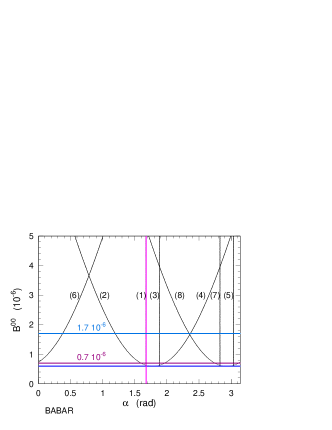
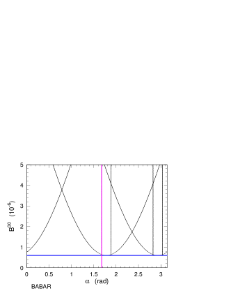
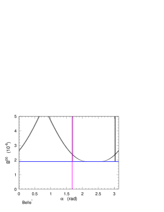
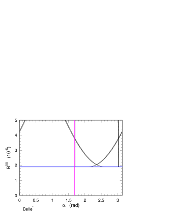
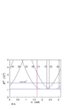
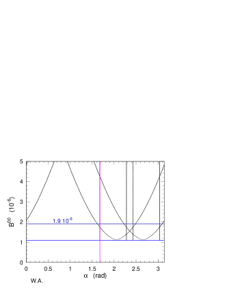
On Fig. 3 are shown the location of the 8 mirror solutions (Table 2) as a function of the value assumed for 00superscript00{\cal B}^{00}. Each set of curves starts at the minimal value given by the reBound. For the sake of clarity, only the solutions obtained with cos(2αeff)2subscript𝛼eff\cos(2\alpha_{\rm eff}) negative are considered, in agreement with the finding of Section 4.1.2. Otherwise, one should also consider another set of six curves, this time starting at the tough Bound.

Four of the mirror solutions given in Table 2 do not depend on 00superscript00{\cal B}^{00}: beside the true solution, they are the solutions (3), (5) and (7). For BABAR as for Belle one of these branching ratio independent solutions is close to the true solution. Whatever 00superscript00{\cal B}^{00}, this nearby mirror solution has a harmful effect on the measurement. However, the current uncertainties on Cππsubscript𝐶𝜋𝜋C_{\pi\pi} and Sππsubscript𝑆𝜋𝜋S_{\pi\pi} are large enough to allow for this mirror solution to drift away swiftly with the coming updates. For the world average, all mirror solutions are harmlessly far apart.

The location of the other four mirror solutions depend on 00superscript00{\cal B}^{00}, because C00subscript𝐶00C_{00} is a multivalued function of this branching ratio. The C00(00)subscript𝐶00superscript00C_{00}({\cal B}^{00}) function drawn on Fig. 2 shows that there exist two values of C00subscript𝐶00C_{00} for a given 00superscript00{\cal B}^{00} and for a given sign of the product cos(2αeff)cos(2α0)2subscript𝛼eff2subscript𝛼0\cos(2\alpha_{\rm eff})\cos(2\alpha_{0}). The three sets of curves on the left hand side are obtained with the upper corresponding values of C00subscript𝐶00C_{00} and the three sets of curves on the right hand side with the lower values of C00subscript𝐶00C_{00} (for cos(2αeff)cos(2α0)2subscript𝛼eff2subscript𝛼0\cos(2\alpha_{\rm eff})\cos(2\alpha_{0}) positive). The curves for the two different C00subscript𝐶00C_{00} bounce back together when 00superscript00{\cal B}^{00} hits the reBound α:l+00subscriptsuperscript00:𝛼limit-froml{\cal B}^{00}_{\alpha:{\rm l}+}.

The worst case scenario is when three mirror solutions gather around the true solution (ie. when 00GLSS:l00similar-to-or-equalssuperscript00subscriptsuperscript00:GLSSl{\cal B}^{00}\simeq{\cal B}^{00}_{\rm GLSS:l}). With BABAR values, because α:l+00GLSS:l00similar-to-or-equalssubscriptsuperscript00:𝛼limit-fromlsubscriptsuperscript00:GLSSl{\cal B}^{00}_{\alpha:{\rm l}+}\simeq{\cal B}^{00}_{\rm GLSS:l} for α=96o𝛼superscript96𝑜\alpha~{}=~{}96^{o}, this happens for 00superscript00{\cal B}^{00} close to the reBound, where one observes that 3 mirror solutions are lumped together with the true solution. In that case, the higher 00superscript00{\cal B}^{00}, the better the measurement of α𝛼\alpha. With Belle, or with the world average values, the worst case scenario is avoided because the GLSS bound is well below the reBound. However, nasty situations where some mirror solutions collide with α𝛼\alpha can still occur. With Belle values, this happens by accident (i.e. for 00GLSS:l00superscript00subscriptsuperscript00:GLSSl{\cal B}^{00}\neq{\cal B}^{00}_{\rm GLSS:l}) for 002.4×10⁶similar-to-or-equalssuperscript002.4superscript106{\cal B}^{00}\simeq 2.4\times 10^{-6}.

Refer to caption Refer to caption Refer to caption Refer to caption Refer to caption Refer to caption

Figure 3: Location of the 8 mirror solutions as a function of 00superscript00{\cal B}^{00}. The six sets of curves refer to BABAR (top), Belle (middle) and the world average (bottom). Each set starts at the minimal value 00=α:l+00superscript00subscriptsuperscript00:𝛼limit-froml{\cal B}^{00}={\cal B}^{00}_{\alpha:{\rm l}+}. Only the solutions obtained with cos(2αeff)2subscript𝛼eff\cos(2\alpha_{\rm eff}) negative (Section 4.1.2) are considered. The curves on the left hand side are obtained with the C00subscript𝐶00C_{00} value corresponding to the upper part of the C00(00)subscript𝐶00superscript00C_{00}({\cal B}^{00}) function (Fig. 2), the ones on the right hand side with the C00subscript𝐶00C_{00} value corresponding to the lower part of the C00(00)subscript𝐶00superscript00C_{00}({\cal B}^{00}) function. The vertical lines drawn on each plot represent the true value of α𝛼\alpha (96osuperscript96𝑜96^{o}) and the mirror solutions (3), (5) and (7) which are independent of 00superscript00{\cal B}^{00}. Four scenarii serve as illustrations in Section 5.2 (W.A. using 00=1.9×10⁶superscript001.9superscript106{\cal B}^{00}=1.9\times 10^{-6}) and Section 5.3 (BABAR, using 00=1.7superscript001.7{\cal B}^{00}=1.7 and 0.7×1060.7superscript1060.7\times 10^{-6}). The corresponding horizontal lines are drawn here to indicate the locations of the 8 mirror solutions.

5.2 Guessestimates for high luminosity (10ab110superscriptab110~{}\mbox{ab}^{-1})

+(106)superscriptabsentsuperscript106{\cal B}^{+-}~{}(10^{-6}) +0(106)superscript0superscript106{\cal B}^{+0}~{}(10^{-6}) 00(106)superscript00superscript106{\cal B}^{00}~{}(10^{-6})
10ab110superscriptab110~{}\mbox{ab}^{-1} 4.55±0.10plus-or-minus4.550.104.55\pm 0.10 5.18±0.18plus-or-minus5.180.185.18\pm 0.18\ 1.9±0.11plus-or-minus1.90.111.9\pm 0.11
1000fb11000superscriptfb11000~{}\mbox{fb}^{-1} 4.55±0.19plus-or-minus4.550.194.55\pm 0.19 5.18±0.32plus-or-minus5.180.325.18\pm 0.32\ 1.9±0.22plus-or-minus1.90.221.9\pm 0.22
Cππsubscript𝐶𝜋𝜋C_{\pi\pi} Sππsubscript𝑆𝜋𝜋S_{\pi\pi} C00subscript𝐶00C_{00}
10ab110superscriptab110~{}\mbox{ab}^{-1} 0.46±0.04plus-or-minus0.460.04-0.46\pm 0.04 0.73±0.03plus-or-minus0.730.03-0.73\pm 0.03 0.8/0.38±0.080.8/-0.38\pm 0.08
1000fb11000superscriptfb11000~{}\mbox{fb}^{-1} 0.46±0.07plus-or-minus0.460.07-0.46\pm 0.07 0.73±0.07plus-or-minus0.730.07-0.73\pm 0.07 0.8/0.38±0.260.8/-0.38\pm 0.26
Table 4: Input values to the fits for the branching ratios, the CP violating asymmetries and their extrapolated errors for 101010 and 1ab11superscriptab11~{}\mbox{ab}^{-1}. The central values are the W.A. ones. The two values quoted for C00subscript𝐶00C_{00} are the ones obtained for cos(2αeff)cos(2α0)2subscript𝛼eff2subscript𝛼0\cos(2\alpha_{\rm eff})\cos(2\alpha_{0}) positive.

The value α=96o𝛼superscript96𝑜\alpha~{}=~{}96^{o} is chosen together with cos(2αeff)2subscript𝛼eff\cos(2\alpha_{\rm eff}) negative (Section 4.1.2). The central values for W.A. are used as inputs and the errors are extrapolated to 10ab110superscriptab110~{}\mbox{ab}^{-1} (Table 4). Such a luminosity gives a number of π0π0superscript𝜋0superscript𝜋0\pi^{0}\pi^{0} events close to 500050005000. This set of parameters is consistent with two different values of C00subscript𝐶00C_{00} as shown Fig. 2, which are equal to 0.800.800.80 and 0.380.38-0.38. The estimated errors for both C00subscript𝐶00C_{00} are taken to be 0.080.080.08.

The result of the fit is shown on Fig. 4 (C00=0.8subscript𝐶000.8C_{00}=0.8) and Fig. 5 (C00=0.38subscript𝐶000.38C_{00}=-0.38). Six of the mirror solutions appear above α=96o𝛼superscript96𝑜\alpha~{}=~{}96^{o}. The domain allowed at more than 5% CL is quite large. Because of that one may be tempted to conclude that ππ𝜋𝜋\pi\pi does not bring much to CKM metrology. However, one should keep in mind that CKM fits receive contributions from numerous measurements. It is thus misleading to compare α(ππ)𝛼𝜋𝜋\alpha(\pi\pi) to all the other measurements taken at once. Furthermore, precisely because one expects the domain in α𝛼\alpha allowed by a global fit to be quite small in the high luminosity area, the low CL values are not anymore relevant. For metrology, what matters then is the sharpness of the 8 peaks. If no mirror solution shows up in the vicinity of the correct α𝛼\alpha value, then ππ𝜋𝜋\pi\pi may contribute to CKM metrology in a very significant way by helping to pinpoint precisely α𝛼\alpha. This is the case for C00=0.8subscript𝐶000.8C_{00}=0.8 where the 8 peaks are sharp, but this is not the case for C00=0.38subscript𝐶000.38C_{00}=-0.38 where the peaks are dull.

Refer to caption Refer to caption

Figure 4: Confidence Level CL(α𝛼\alpha)=Prob(χmin2,1)subscriptsuperscript𝜒2min1(\chi^{2}_{\rm min},1) obtained for W.A. central values at a luminosity of 10ab110superscriptab110~{}\mbox{ab}^{-1} when performing a direct fit with a fine-grain exploration of the parameter space (left). The value chosen for C00subscript𝐶00C_{00} is 0.80.80.8. One observes the 8 mirror solutions showing up as 8 CL=1 peaks. The right plot is a zoom around the true solution α=96o𝛼superscript96𝑜\alpha~{}=~{}96^{o} (1.67rad1.67rad1.67~{}\rm rad). The presence on the left hand side of the nearby mirror solution (2) makes the CL curve asymmetrical. The 32% CL is reached at α=1.67±σ±𝛼plus-or-minus1.67subscript𝜎plus-or-minus\alpha~{}=~{}{1.67}\pm\sigma_{\pm} with σ+=0.07subscript𝜎0.07\sigma_{+}=0.07 and σ=0.08subscript𝜎0.08\sigma_{-}=0.08 (radians). The doted line represents CL(α𝛼\alpha) for a luminosity of 1000fb11000superscriptfb11000~{}\mbox{fb}^{-1}. In that case, one practically looses all constraints on the left hand side: the mirror solution (2) is too close to be resolved. However, the error on the right hand side remains useful: σ=0.19subscript𝜎0.19\sigma_{-}=0.19.

A zoom around α=96o𝛼superscript96𝑜\alpha~{}=~{}96^{o} is shown on Fig. 4 (right) in plain line. Because of the nearby mirror solution (2), the CL curve is not symmetrical. Defining σ±subscript𝜎plus-or-minus\sigma_{\pm} by CL(1.67±σ±)=32%plus-or-minus1.67subscript𝜎plus-or-minuspercent32(1.67\pm\sigma_{\pm})=32\% one gets σ+=0.07subscript𝜎0.07\sigma_{+}=0.07 and σ=0.08subscript𝜎0.08\sigma_{-}=0.08. The negative error blows up fast with decreasing luminosity, because the fit is quickly not able anymore to resolve the true solution from the mirror solution (2). The positive error scales almost with the square root of the luminosity because the CL is almost at zero down the pic. The CL(α)𝛼(\alpha) for a luminosity of 1000fb11000superscriptfb11000~{}\mbox{fb}^{-1} is shown as well in dotted line. For this case the positive error σ=0.19subscript𝜎0.19\sigma_{-}=0.19 is slightly smaller than the (ill-defined) actual precision on α𝛼\alpha from the global CKM fit (=0.23absent0.23=0.23). Obviously, before then, the measurement of ΔmsΔsubscript𝑚𝑠\Delta m_{s} by the Tevatron experiments will have changed the global CKM picture.

Refer to caption Refer to caption

Figure 5: Confidence Level CL(α𝛼\alpha)=Prob(χmin2,1)subscriptsuperscript𝜒2min1(\chi^{2}_{\rm min},1) obtained for W.A. central values at a luminosity of 10ab110superscriptab110~{}\mbox{ab}^{-1} when performing a direct fit with a fine-grain exploration of the parameter space. The value chosen for C00subscript𝐶00C_{00} is 0.380.38-0.38. The CL curves obtained in that case are to be compared with the ones if Fig. 4 (C00=0.8subscript𝐶000.8C_{00}=0.8). In the present case, the peaks merged partly and are much less pronounced.

5.3 Two scenarii at 500fb1500superscriptfb1500~{}\mbox{fb}^{-1} for BABAR

+(106)superscriptabsentsuperscript106{\cal B}^{+-}~{}(10^{-6}) +0(106)superscript0superscript106{\cal B}^{+0}~{}(10^{-6}) 00(106)superscript00superscript106{\cal B}^{00}~{}(10^{-6})
scenario I 4.7±0.26plus-or-minus4.70.264.7\pm 0.26 5.5±0.43plus-or-minus5.50.435.5\pm 0.43\ 0.7±0.29plus-or-minus0.70.290.7\pm 0.29
scenario II 4.7±0.26plus-or-minus4.70.264.7\pm 0.26 5.5±0.43plus-or-minus5.50.435.5\pm 0.43\ 1.7±0.29plus-or-minus1.70.291.7\pm 0.29
Cππsubscript𝐶𝜋𝜋C_{\pi\pi} Sππsubscript𝑆𝜋𝜋S_{\pi\pi} C00subscript𝐶00C_{00}
scenario I 0.19±0.09plus-or-minus0.190.09-0.19\pm 0.09 0.40±0.10plus-or-minus0.400.10-0.40\pm 0.10 0.47±1.29plus-or-minus0.471.290.47\pm 1.29
scenario II 0.19±0.09plus-or-minus0.190.09-0.19\pm 0.09 0.40±0.10plus-or-minus0.400.10-0.40\pm 0.10 0.29±0.58plus-or-minus0.290.580.29\pm 0.58
Table 5: Input values to the fits for the branching ratios, the CP violating asymmetries and their extrapolated errors. Scenarii I and II use the BABAR values for +superscriptabsent{\cal B}^{+-}, +0superscript0{\cal B}^{+0}, Cππsubscript𝐶𝜋𝜋C_{\pi\pi} and Sππsubscript𝑆𝜋𝜋S_{\pi\pi} and two distinct 00superscript00{\cal B}^{00} guesses.

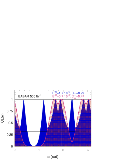
Now, only the BABAR central values are considered, at a luminosity of 500fb1500superscriptfb1500~{}\mbox{fb}^{-1} which is planned to be reached in 2006 by BABAR. Considering the upper left plot on Fig. 3, one considers two scenarii for 00superscript00{\cal B}^{00}. The worst case scenarii are obtained when several mirror solutions gather around the true solution, staying about one σ[α]𝜎delimited-[]𝛼\sigma[\alpha] away. With BABAR values, this happens for 00superscript00{\cal B}^{00} close to the reBound value α:l+00=0.6×10⁶subscriptsuperscript00:𝛼limit-froml0.6superscript106{\cal B}^{00}_{\alpha:{\rm l}+}=0.6\times 10^{-6}, where 3 mirror solutions are lumped together with the true solution. As discussed in Section 4.3 this happens because αeffsubscript𝛼eff\alpha_{\rm eff} being close to α𝛼\alpha, the reBound is close to the GLSS bound where the mirror solutions are exactly degenerate. To show the effect, one considers a scenario with the barely acceptable value 00=0.7×10⁶superscript000.7superscript106{\cal B}^{00}=0.7\times 10^{-6}: this is the scenario I. Scenario II is one where, taking the opposite stand, 00superscript00{\cal B}^{00} is far from the reBound. The degeneracy between the mirror solutions is then lifted which lets presume that the measurement of α𝛼\alpha will be easier. The value 00=1.7×10⁶superscript001.7superscript106{\cal B}^{00}=1.7\times 10^{-6} is chosen for this case.

The values used for these two scenarii are presented in Table 5. The result of the fits are shown Fig. 6. A zoom of the fits around the true value of α𝛼\alpha is displayed on the right.

Refer to caption Refer to caption

Figure 6: Confidence Level CL(α𝛼\alpha)=Prob(χmin2,1)\chi^{2}_{\rm min},1) obtained for scenario I and scenario II. The luminosity is 500fb1500superscriptfb1500~{}\mbox{fb}^{-1} and α=96o𝛼superscript96𝑜\alpha~{}=~{}96^{o}. The right plot is a zoom around the value α=96o𝛼superscript96𝑜\alpha~{}=~{}96^{o} (1.67rad1.67rad1.67~{}\rm rad) for 00=0.7×10⁶superscript000.7superscript106{\cal B}^{00}=0.7\times 10^{-6} (dotted line) and 00=1.7×10⁶superscript001.7superscript106{\cal B}^{00}=1.7\times 10^{-6} (plain line).

Whereas, in scenario II, the larger value of the branching ratio 00superscript00{\cal B}^{00} leaves some power to the analysis, in scenario I, the vicinity of the mirror solutions deprives the analysis of most of its interest.

6 Standard Model Tests: the (00,C00)superscript00subscript𝐶00({\cal B}^{00},C_{00}) plot

The above discussion offers a perspective on the future capabilities of ππ𝜋𝜋\pi\pi analysis to constraint the angle α𝛼\alpha: everything can happen in the few coming years, including a precise measurement of α𝛼\alpha from the Bππ𝐵𝜋𝜋B\to\pi\pi decays.

Testing the Standard Model is a different topic. Although this question can be addressed by comparing the constraints on α𝛼\alpha from the standard CKM fit to the ones obtained from Bππ𝐵𝜋𝜋B\to\pi\pi decays, it is a clumsy way to proceed. Indeed, one has to deal with the mirror solutions which are irrelevant when one is only willing to know whether or not the Standard Model can accomodate the set of six measurements +superscriptabsent{\cal B}^{+-}, +0superscript0{\cal B}^{+0}, 00superscript00{\cal B}^{00}, Cππsubscript𝐶𝜋𝜋C_{\pi\pi}, Sππsubscript𝑆𝜋𝜋S_{\pi\pi} and C00subscript𝐶00C_{00} knowing α𝛼\alpha from other measurements. Since the last precise measurements are going to be 00superscript00{\cal B}^{00} and C00subscript𝐶00C_{00} (the latter being still out of reach) it is appropriate to probe the Standard Model by considering the (00,C00)superscript00subscript𝐶00({\cal B}^{00},C_{00}) plane.

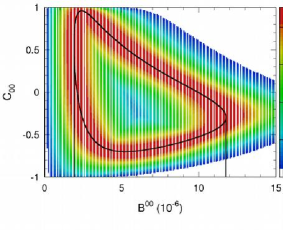
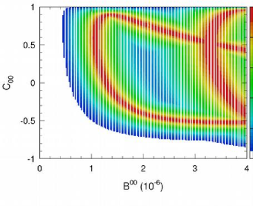
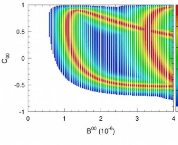
The C00(00)subscript𝐶00superscript00C_{00}({\cal B}^{00}) function introduced in Section 4.2 has shown the possible contour, for BABAR, Belle and W.A., of C00subscript𝐶00C_{00} as a function of 00superscript00{\cal B}^{00} (Fig. 2). Here is now presented the plane (00,C00superscript00subscript𝐶00{\cal B}^{00},C_{00}) when a fit is performed using +superscriptabsent{\cal B}^{+-}, +0superscript0{\cal B}^{+0}, Cππsubscript𝐶𝜋𝜋C_{\pi\pi}, Sππsubscript𝑆𝜋𝜋S_{\pi\pi} and α𝛼\alpha, in order to evaluate the CL at each point. To look at this plane is a proper way to handle data because no bound is needed, nor dealing with mirror solutions. The results for the three experimental cases are presented on Fig. 7 for the present luminosity and α=96o𝛼superscript96𝑜\alpha~{}=~{}96^{o} with the curves of Fig. 2 superimposed. Considering the allowed region (00<4×10⁶superscript004superscript106{\cal B}^{00}<4\times 10^{-6}), one observes that there is practically no constraints on C00subscript𝐶00C_{00}, neither for BABAR, Belle or W.A. Similarly, with the present level of knowledge, any value of 00superscript00{\cal B}^{00} can be accomodated by the Standard Model, except exceedingly small ones.
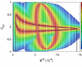
Refer to caption Refer to caption Refer to caption

Figure 7: The (00,C00)superscript00subscript𝐶00({\cal B}^{00},C_{00}) plane is presented for BABAR (left), Belle (middle) and W.A. (right), using the actual luminosity and α=96o𝛼superscript96𝑜\alpha~{}=~{}96^{o}. The curves superimposed are the ones given by Eq.(35) for cos(2αeff)2subscript𝛼eff\cos(2\alpha_{\rm eff}) negative (see Fig. 2).

Figure 8 represent the plane (00,C00superscript00subscript𝐶00{\cal B}^{00},C_{00}) considering the W.A. results, for a luminosity of 500500500 and 1000fb11000superscriptfb11000~{}\mbox{fb}^{-1}. To rule out the Standard Model would imply an accurate measurement of a large negative value of C00subscript𝐶00C_{00} and/or a very small value of 00superscript00{\cal B}^{00}.

Refer to caption Refer to caption

Figure 8: The (00,C00)superscript00subscript𝐶00({\cal B}^{00},C_{00}) plane is presented using the world average branching ratios and CP parameters, for 500fb1500superscriptfb1500~{}\mbox{fb}^{-1} (left) and 1000fb11000superscriptfb11000~{}\mbox{fb}^{-1} (right).

7 Conclusion

The constraints on the angle α𝛼\alpha are revisited, considering the three branching ratios +superscriptabsent{\cal B}^{+-}, +0superscript0{\cal B}^{+0} and 00superscript00{\cal B}^{00}, and the three CP parameters Cππsubscript𝐶𝜋𝜋C_{\pi\pi}, Sππsubscript𝑆𝜋𝜋S_{\pi\pi} and C00subscript𝐶00C_{00}. A new bound is established on 00superscript00{\cal B}^{00} taking advantage of the constraints on α𝛼\alpha available from the standard CKM fit. The function C00(00)subscript𝐶00superscript00C_{00}({\cal B}^{00}) is introduced and the use of the (00,C00)superscript00subscript𝐶00({\cal B}^{00},C_{00}) plane is advocated as a means to probe new physics, when the measurement of C00subscript𝐶00C_{00} will be available. The Grossman-Quinn bound is discussed and a compact formula is provided which highlights its domain of validity.

When considering BABAR results, three cases can be considered: 1) if 00superscript00{\cal B}^{00} reaches exactly its lower bound, there is no ambiguity for α𝛼\alpha (but this is academic), 2) if 00superscript00{\cal B}^{00} is only close to its lower bound, the locations of the mirror solutions are varying rapidly as a function of 00superscript00{\cal B}^{00} and the evaluation of α𝛼\alpha becomes difficult, 3) if 00superscript00{\cal B}^{00} is far enough from the lower bound, the degeneracy between the mirror solutions tend to be lifted and the measurement of α𝛼\alpha may become feasible with only a medium statistics. The current period is very exciting, anything can happen in the next three years: including a rather precise determination of α𝛼\alpha.

The introduction of the (00,C00superscript00subscript𝐶00{\cal B}^{00},C_{00}) plane in order to test the Standard Model shows that it will be difficult to rule out this latter.

References

  • [1] M. Gronau and D. London, “Isospin analysis of CP𝐶𝑃CP asymmetries in B decays”, Phys. Rev. Lett. 65, 3381, (1990).
  • [2] P.F. Harrison et H.R. Quinn, editeurs, “The BABAR physics book”, SLAC-R-504 (1998).
  • [3] A. Höcker, H. Lacker, M. Pivk et L. Roos, “Interpreting CP𝐶𝑃CP Asymmetries in B0π+πsuperscript𝐵0superscript𝜋superscript𝜋B^{0}\to{\pi^{+}\pi^{-}} Decays”, LAL 02-103 (October 2002).
  • [4] A. Ali, E. Lunghi, A. Parkhomenko, “An analysis of the time dependent CP asymmetry in Bππ𝐵𝜋𝜋B\to\pi\pi decays in the Standard Model”, DESY-04-036, ZU-TH-02-04 (March 2004). Submitted to Eur.Phys.J.C, hep-ph/0403275.
  • [5] M. Pivk and F.R. Le Diberder, “𝒫slotsubscript𝒫𝑠𝑙𝑜𝑡\hbox{${}_{s}$}{\cal P}lot: a statistical tool to unfold data distributions”, physics/0402083, (February 2004).
  • [6] M. Pivk, Thèse de l’Université Paris VII, May 2003 (in French),
    BABAR-THESIS-03/012,
    http://tel.ccsd.cnrs.fr/documents/archives0/00/00/29/91/index_fr.html
  • [7] HFAG Web page, http://www.slac.stanford.edu/xorg/hfag/triangle/index.html
  • [8] BABAR  collaboration, B. Aubert et al., “ Measurements of branching fractions and CP violating asymmetries in B0π+π,K+π,K+Ksuperscript𝐵0superscript𝜋superscript𝜋superscript𝐾superscript𝜋superscript𝐾superscript𝐾B^{0}\to\pi^{+}\pi^{-},K^{+}\pi^{-},K^{+}K^{-} decays”, Phys. Rev. Lett. 89, 281802 hep-ex/0207055, (July 2002).
  • [9] BABAR  collaboration, B. Aubert et al., “Observation of the decay B+π+π0superscript𝐵superscript𝜋superscript𝜋0B^{+}\to\pi^{+}{\pi^{0}}, study of B+K±π0superscript𝐵superscript𝐾plus-or-minussuperscript𝜋0B^{+}\to K^{\pm}{\pi^{0}}, and search for B0π0π0superscript𝐵0superscript𝜋0superscript𝜋0B^{0}\to\pi^{0}\pi^{0}”, Phys. Rev. Lett. 91:021801, hep-ex/0303028, (March 2003).
  • [10] BABAR  collaboration, B. Aubert et al., “Observation of a significant excess of π0π0superscript𝜋0superscript𝜋0{\pi^{0}}{\pi^{0}} events in B meson decays”, Phys. Rev. Lett. 91:241801, hep-ex/0308012, (August 2003).
  • [11] Belle collaboration, Y. Chao et al., “Improved Measurements of Branching Fractions in BKπ,ππ,KK𝐵𝐾𝜋𝜋𝜋𝐾𝐾B\to K\pi,\pi\pi,KK decays”, hep-ex/0311061, (Novembre 2003).
  • [12] ”CKM unitarity angles α(ϕ2)𝛼subscriptitalic-ϕ2\alpha(\phi_{2}) and γ(ϕ3)𝛾subscriptitalic-ϕ3\gamma(\phi_{3})”, talk given by H. Jawahery at Lepton-Photon 2003.
  • [13] Belle collaboration, K. Abe et al., “Observation of large CP violation and evidence for direct CP violation in B0π+πsuperscript𝐵0superscript𝜋superscript𝜋B^{0}\to{\pi^{+}\pi^{-}}\ decays”, hep-ex/0401029 (January 2004).
  • [14] CLEO collaboration (A. Bornheim et al.), “Measurements of Charmless Hadronic Two-Body B Meson Decays and the ratio (BDK)𝐵𝐷𝐾{\cal B}(B\to DK)/(BDπ)𝐵𝐷𝜋{\cal B}(B\to D\pi)”, hep-ex/0302026 (February 2003).
  • [15] Particle Data Group (K. Hagiwara et al.), Phys. Rev. D66, 010001 (2002)
  • [16] CKMfitter Web page, http://www.slac.stanford.edu/xorg/ckmfitter/
  • [17] Y. Grossman and H. R. Quinn, “Bounding the Effect of Penguin Diagrams in acp(B0π+π)subscript𝑎cpsuperscript𝐵0superscript𝜋superscript𝜋a_{\rm cp}(B^{0}\rightarrow\pi^{+}\pi^{-})”, Phys. Rev. D58: 017504 (1998).
  • [18] J. Charles, “Taming the Penguin in the Bd0(t)π+πsubscriptsuperscript𝐵0𝑑𝑡superscript𝜋superscript𝜋B^{0}_{d}(t)\rightarrow\pi^{+}\pi^{-} CP-Asymmetry: Observables and Minimal Theoretical Input”, Phys. Rev. D59: 054007 (1999).
  • [19] M. Gronau, D. London, N. Sinha, R. Sinha, “Improving Bounds on Penguin Pollution in Bππ𝐵𝜋𝜋B\rightarrow\pi\pi”, Phys. Lett. B514: 315 (2001).
  • [20] A. Höcker, H. Lacker, S. Laplace and F. R. Le Diberder, Eur. Phys. J. C21, 225, hep-ph/0104062 (2001).