OSU-HEP-03-10

August 2003

Anomalous U​(1)π‘ˆ1U(1) Symmetry and
Lepton Flavor Violation

K.S. Babu,111E-mail address: babu@okstate.edu Ts. Enkhbat222E-mail address: enkhbat@okstate.edu and I. Gogoladze333On a leave of absence from: Andronikashvili Institute of Physics, GAS, 380077 Tbilisi, Georgia.
E-mail address: ilia@hep.phy.okstate.edu

Department of Physics, Oklahoma State University
Stillwater, OKΒ 74078, USA

We show that in a large class of models based on anomalous U​(1)π‘ˆ1U(1) symmetry which addresses the fermion mass hierarchy problem, leptonic flavor changing processes are induced that are in the experimentally interesting range. The flavor violation occurs through the renormalization group evolution of the soft SUSY breaking parameters between the string scale and the U​(1)Aπ‘ˆsubscript1𝐴U(1)_{A} breaking scale. We derive general expressions for the evolution of these parameters in the presence of higher dimensional operators. Several sources for the flavor violation are identified: flavor–dependent contributions to the soft masses from the U​(1)Aπ‘ˆsubscript1𝐴U(1)_{A} gaugino, scalar mass corrections proportional to the trace of U​(1)Aπ‘ˆsubscript1𝐴U(1)_{A} charge, non–proportional A𝐴A–terms from vertex corrections, and the U​(1)Aπ‘ˆsubscript1𝐴U(1)_{A} D𝐷D–term. Quantitative estimates for the decays ΞΌβ†’eβ€‹Ξ³β†’πœ‡π‘’π›Ύ\mu\rightarrow e\gamma and Ο„β†’ΞΌβ€‹Ξ³β†’πœπœ‡π›Ύ\tau\rightarrow\mu\gamma are presented in supergravity models which accommodate the relic abundance of neutralino dark matter.

1 Introduction

The Standard Model, while highly successful in explaining all experimental data, does not provide an explanation for the observed hierarchy in the masses and mixings of quarks and leptons. Extended symmetries are often speculated to address this problem. Family–dependent U​(1)π‘ˆ1U(1) symmetry is a widely studied extension. An attractive scenario is the Froggatt–Nielsen scheme [1]. In this scenario all the Yukawa couplings are assumed to be of order one, but the ones which generate the light fermion masses arise only as nonrenormalizable operators suppressed by powers of a small parameter Ο΅β‰‘βŸ¨S⟩/Mitalic-Ο΅delimited-βŸ¨βŸ©π‘†π‘€\epsilon\equiv\langle S\rangle/M, where ⟨S⟩delimited-βŸ¨βŸ©π‘†\langle S\rangle is the flavor symmetry breaking order parameter and M𝑀M is a more fundamental mass scale. With the flavor U​(1)π‘ˆ1U(1) charges of fermions differing only by order one, large hierarchy factors, such as mu/mt∼10βˆ’6similar-tosubscriptπ‘šπ‘’subscriptπ‘šπ‘‘superscript106m_{u}/m_{t}\sim 10^{-6}, are explained.

A natural origin for the flavor U​(1)π‘ˆ1U(1) symmetry is the anomalous U​(1)Aπ‘ˆsubscript1𝐴U(1)_{A} gauge symmetry of string theory [2]. The small expansion parameter Ο΅italic-Ο΅\epsilon arises in a natural way in anomalous U​(1)π‘ˆ1U(1) models through the Fayet–Iliopoulos term induced by the gravitational anomaly [3]. Such models have been extensively studied in the literature for understanding the fermion mass hierarchy puzzle [4, 5]. The purpose of this paper is to address flavor changing neutral currents in this class of models.

In the presence of low energy supersymmetry (SUSY), a family–dependent anomalous U​(1)Aπ‘ˆsubscript1𝐴U(1)_{A} symmetry will induce flavor changing processes, even when there is no flavor violation in the soft SUSY breaking parameters at the fundamental scale – taken to be the string scale. Such violations will be generated through the renormalization group evolution (RGE) of the SUSY breaking parameters between Ms​t​r​i​n​gsubscriptπ‘€π‘ π‘‘π‘Ÿπ‘–π‘›π‘”M_{string} and the U​(1)Aπ‘ˆsubscript1𝐴U(1)_{A} breaking scale ⟨S⟩delimited-βŸ¨βŸ©π‘†\langle S\rangle. We derive general expressions for the evolution of these parameters in the presence of higher dimensional operators. Our results can be applied to a wide class of Froggatt–Nielsen models. We have found several sources of flavor violation. In the momentum interval ⟨SβŸ©β‰€ΞΌβ‰€Ms​t​r​i​n​gdelimited-βŸ¨βŸ©π‘†πœ‡subscriptπ‘€π‘ π‘‘π‘Ÿπ‘–π‘›π‘”\langle S\rangle\leq\mu\leq M_{string}, the U​(1)Aπ‘ˆsubscript1𝐴U(1)_{A} gaugino is active and will contribute differently to the soft masses of different families. Because Tr​U​(1)ATrπ‘ˆsubscript1𝐴{\rm Tr}U(1)_{A} is not zero in anomalous U​(1)π‘ˆ1U(1) models, there are nonuniversal RGE contributions to the soft scalar masses arising from the D𝐷D–term proportional to the respective flavor charges. Furthermore, the trilinear A𝐴A–terms will receive vertex corrections from the U​(1)Aπ‘ˆsubscript1𝐴U(1)_{A} gaugino that are not proportional to the respective Yukawa couplings. In addition to these RGE effects, upon symmetry breaking, the D𝐷D–term associated with the U​(1)Aπ‘ˆsubscript1𝐴U(1)_{A} will also induce nonuniversal masses for the sfermions [6]–[8].

In this paper we investigate the combined effects of nonuniversality for lepton flavor violating (LFV) decays ΞΌβ†’eβ€‹Ξ³β†’πœ‡π‘’π›Ύ\mu\rightarrow e\gamma and Ο„β†’ΞΌβ€‹Ξ³β†’πœπœ‡π›Ύ\tau\rightarrow\mu\gamma in a class of anomalous U​(1)Aπ‘ˆsubscript1𝐴U(1)_{A} models. Quantitative predictions for the branching ratios are presented in two specific models of fermion mass hierarchy. We find that the branching ratio for ΞΌβ†’eβ€‹Ξ³β†’πœ‡π‘’π›Ύ\mu\rightarrow e\gamma is around the current experimental limit, while Ο„β†’ΞΌβ€‹Ξ³β†’πœπœ‡π›Ύ\tau\rightarrow\mu\gamma may be accessible in the future. In our analysis we also include the right–handed neutrino–induced LFV effects, which have been widely studied in the literature [9]–[11]. These effects turn out to be significant in some but not all cases that we study. In fact, within our framework, if leptogenesis is assumed to be the source of the observed cosmological baryon asymmetry [12], it turns out that the right–handed neutrino induced LFV effects are negligible. Related effects from SUSY GUT thresholds for LFV have been studied in Ref. [13]. The flavor violating effects are more prominent in the leptonic sector compared to the quark sector since quark flavor violation is diluted somewhat by the gluino focusing effects which arise during the evolution of the SUSY breaking parameters below the U​(1)Aπ‘ˆsubscript1𝐴U(1)_{A} breaking scale. This is especially so when the SUSY parameter are chosen, as we do, such that the lightest neutralino is the dark matter with an acceptable cosmological abundance.

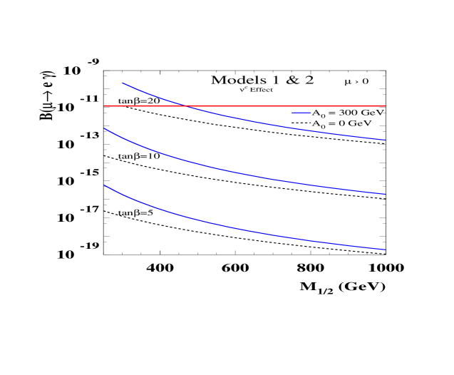
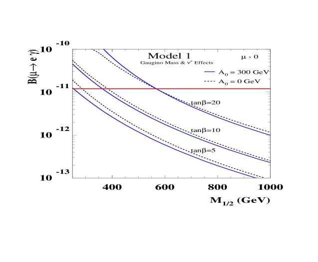
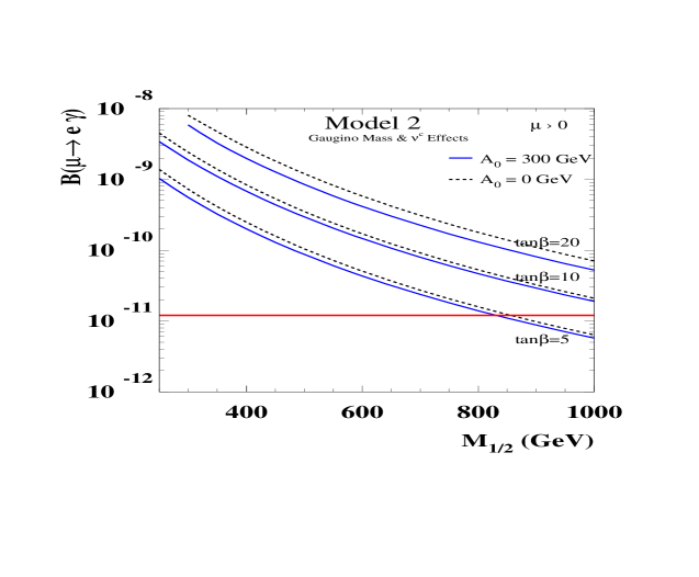
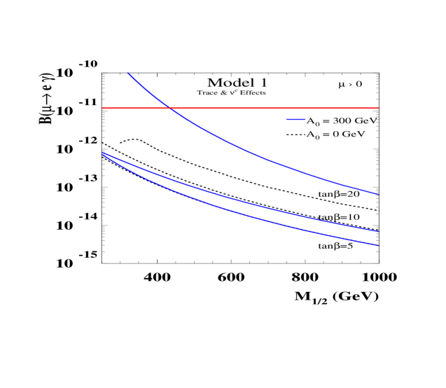
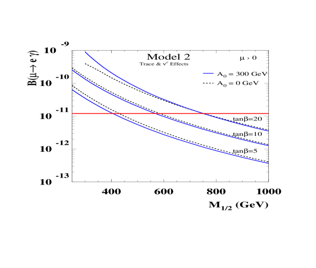
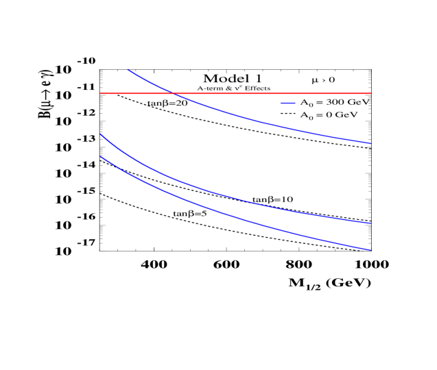
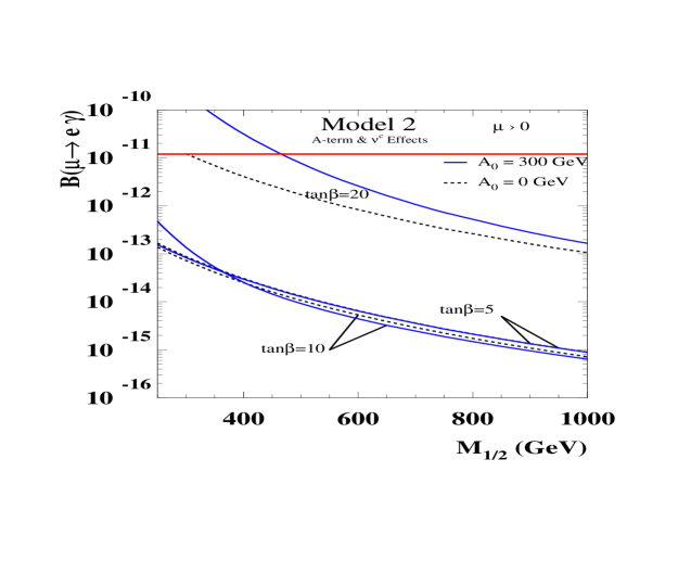
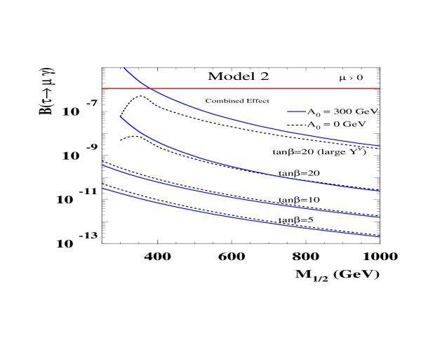
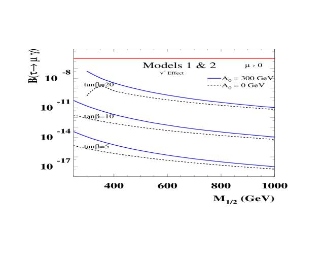
The structure of the paper is as follows. In Section 2 we introduce our models. In 2.1 we describe our models of fermion mass hierarchy, in 2.2 we present the details of anomalous U​(1)π‘ˆ1U(1) models. In 2.3 we present our fermion mass fits for two models, Model 1 and Model 2. In 2.4 we discuss baryogenesis through leptogenesis in these models. In Section 3 we derive generalized expressions for the evolution of the soft SUSY breaking parameters appropriate for a class of Froggatt–Nielsen models. Section 4 is devoted to the numerical analysis of the branching ratios for the processes ΞΌβ†’eβ€‹Ξ³β†’πœ‡π‘’π›Ύ\mu\rightarrow e\gamma and Ο„β†’ΞΌβ€‹Ξ³β†’πœπœ‡π›Ύ\tau\rightarrow\mu\gamma. In 4.1 we outline the qualitative features of flavor violation arising from various sources. 4.2 has our numerical fits. Figures 3 and 4 show our results for the branching ratios for ΞΌβ†’eβ€‹Ξ³β†’πœ‡π‘’π›Ύ\mu\rightarrow e\gamma in the two models of fermion masses. In 4.3 we address the D𝐷D-term splitting problem. Our conclusions are given in Section 5.

2 Fermion Mass Matrices and Anomalous U​(1)Aπ‘ˆsubscript1𝐴U(1)_{A} Flavor Symmetry

In this section we present two specific models of fermion mass hierarchy based on a flavor–dependent anomalous U​(1)Aπ‘ˆsubscript1𝐴U(1)_{A} symmetry using the Froggatt–Nielsen mechanism [1]. The U​(1)Aπ‘ˆsubscript1𝐴U(1)_{A} symmetry is broken by an MSSM singlet flavon filed S𝑆S slightly below the string scale (Ms​tsubscript𝑀𝑠𝑑M_{st}). This provides the small expansion parameter Ο΅=⟨S⟩/Ms​titalic-Ο΅delimited-βŸ¨βŸ©π‘†subscript𝑀𝑠𝑑\epsilon=\langle S\rangle/M_{st} needed for explaining the fermion mass hierarchy. We also present explicit models of anomalous U​(1)Aπ‘ˆsubscript1𝐴U(1)_{A} symmetry.

2.1 Fermion Mass Hierarchy

A general form of the superpotential which can explain the fermion masses and mixing hierarchy through the Froggatt–Nielsen mechanism has the form

Wπ‘Š\displaystyle W =\displaystyle= yi​juni​ju!​Qi​ujc​Hu​(SMs​t)ni​ju+yi​jdni​jd!​Qi​djc​Hd​(SMs​t)ni​jdsuperscriptsubscript𝑦𝑖𝑗𝑒subscriptsuperscript𝑛𝑒𝑖𝑗subscript𝑄𝑖superscriptsubscript𝑒𝑗𝑐subscript𝐻𝑒superscript𝑆subscript𝑀𝑠𝑑subscriptsuperscript𝑛𝑒𝑖𝑗superscriptsubscript𝑦𝑖𝑗𝑑subscriptsuperscript𝑛𝑑𝑖𝑗subscript𝑄𝑖superscriptsubscript𝑑𝑗𝑐subscript𝐻𝑑superscript𝑆subscript𝑀𝑠𝑑subscriptsuperscript𝑛𝑑𝑖𝑗\displaystyle\frac{y_{ij}^{u}}{n^{u}_{ij}!}Q_{i}u_{j}^{c}H_{u}\left(\frac{S}{M_{st}}\right)^{n^{u}_{ij}}+\frac{y_{ij}^{d}}{n^{d}_{ij}!}Q_{i}d_{j}^{c}H_{d}\left(\frac{S}{M_{st}}\right)^{n^{d}_{ij}} (1)
+\displaystyle+ yi​jeni​je!​Li​ejc​Hd​(SMs​t)ni​je+yi​jΞ½ni​jΞ½!​Li​νjc​Hu​(SMs​t)ni​jΞ½superscriptsubscript𝑦𝑖𝑗𝑒subscriptsuperscript𝑛𝑒𝑖𝑗subscript𝐿𝑖superscriptsubscript𝑒𝑗𝑐subscript𝐻𝑑superscript𝑆subscript𝑀𝑠𝑑subscriptsuperscript𝑛𝑒𝑖𝑗superscriptsubscriptπ‘¦π‘–π‘—πœˆsubscriptsuperscriptπ‘›πœˆπ‘–π‘—subscript𝐿𝑖subscriptsuperscriptπœˆπ‘π‘—subscript𝐻𝑒superscript𝑆subscript𝑀𝑠𝑑subscriptsuperscriptπ‘›πœˆπ‘–π‘—\displaystyle\frac{y_{ij}^{e}}{n^{e}_{ij}!}L_{i}e_{j}^{c}H_{d}\left(\frac{S}{M_{st}}\right)^{n^{e}_{ij}}+\frac{y_{ij}^{\nu}}{n^{\nu}_{ij}!}L_{i}\nu^{c}_{j}H_{u}\left(\frac{S}{M_{st}}\right)^{n^{\nu}_{ij}}
+\displaystyle+ MRi​j​νic​νjc​(SMs​t)ni​jΞ½c+μ​Hu​Hd,subscriptsubscript𝑀𝑅𝑖𝑗subscriptsuperscriptπœˆπ‘π‘–subscriptsuperscriptπœˆπ‘π‘—superscript𝑆subscript𝑀𝑠𝑑subscriptsuperscript𝑛superscriptπœˆπ‘π‘–π‘—πœ‡subscript𝐻𝑒subscript𝐻𝑑\displaystyle{M_{R}}_{ij}\nu^{c}_{i}\nu^{c}_{j}\left(\frac{S}{M_{st}}\right)^{n^{\nu^{c}}_{ij}}+\mu H_{u}H_{d}\,,

where i,j=(1, 2, 3)𝑖𝑗123i,j=(1,\,2,\,3) are family indices, ni​jusubscriptsuperscript𝑛𝑒𝑖𝑗{n^{u}_{ij}}, ni​jdsubscriptsuperscript𝑛𝑑𝑖𝑗{n^{d}_{ij}}, ni​jesubscriptsuperscript𝑛𝑒𝑖𝑗{n^{e}_{ij}}, ni​jΞ½subscriptsuperscriptπ‘›πœˆπ‘–π‘—{n^{\nu}_{ij}} and ni​jΞ½csubscriptsuperscript𝑛superscriptπœˆπ‘π‘–π‘—n^{\nu^{c}}_{ij} are positive integers fixed by the choice of U​(1)Aπ‘ˆsubscript1𝐴U(1)_{A} charge assignment. yi​jusubscriptsuperscript𝑦𝑒𝑖𝑗y^{u}_{ij} etc. are Yukawa coupling coefficients which are all taken to be of order one. Here MRsubscript𝑀𝑅M_{R} is the right-handed (Ξ½icsubscriptsuperscriptπœˆπ‘π‘–\nu^{c}_{i}) neutrino mass scale. We use the standard notation for the MSSM fields.

The soft supersymmetry breaking terms which will induce LFV have the form given by

βˆ’Ls​o​f​tsubscriptLπ‘ π‘œπ‘“π‘‘\displaystyle-\textit{L}_{soft} =\displaystyle= {ai​juni​ju!Q~iu~jcHu(SMs​t)ni​ju+ai​jdni​jd!Q~id~jcHd(SMs​t)ni​jd\displaystyle\left\{\frac{a_{ij}^{u}}{n^{u}_{ij}!}\tilde{Q}_{i}\tilde{u}_{j}^{c}H_{u}\left(\frac{S}{M_{st}}\right)^{n^{u}_{ij}}+\frac{a_{ij}^{d}}{n^{d}_{ij}!}\tilde{Q}_{i}\tilde{d}_{j}^{c}H_{d}\left(\frac{S}{M_{st}}\right)^{n^{d}_{ij}}\right. (2)
+\displaystyle+ ai​jeni​je!​L~i​e~jc​Hd​(SMs​t)ni​je+ai​jΞ½ni​jΞ½!​L~i​ν~jc​Hu​(SMs​t)ni​jΞ½+B′​MRi​j​ν~ic​ν~jc​(SMs​t)ni​jΞ½csuperscriptsubscriptπ‘Žπ‘–π‘—π‘’subscriptsuperscript𝑛𝑒𝑖𝑗subscript~𝐿𝑖superscriptsubscript~𝑒𝑗𝑐subscript𝐻𝑑superscript𝑆subscript𝑀𝑠𝑑subscriptsuperscript𝑛𝑒𝑖𝑗superscriptsubscriptπ‘Žπ‘–π‘—πœˆsubscriptsuperscriptπ‘›πœˆπ‘–π‘—subscript~𝐿𝑖subscriptsuperscript~πœˆπ‘π‘—subscript𝐻𝑒superscript𝑆subscript𝑀𝑠𝑑subscriptsuperscriptπ‘›πœˆπ‘–π‘—superscript𝐡′subscriptsubscript𝑀𝑅𝑖𝑗subscriptsuperscript~πœˆπ‘π‘–subscriptsuperscript~πœˆπ‘π‘—superscript𝑆subscript𝑀𝑠𝑑subscriptsuperscript𝑛superscriptπœˆπ‘π‘–π‘—\displaystyle\frac{a_{ij}^{e}}{n^{e}_{ij}!}\tilde{L}_{i}\tilde{e}_{j}^{c}H_{d}\left(\frac{S}{M_{st}}\right)^{n^{e}_{ij}}+\frac{a_{ij}^{\nu}}{n^{\nu}_{ij}!}\tilde{L}_{i}{\tilde{\nu}}^{c}_{j}H_{u}\left(\frac{S}{M_{st}}\right)^{n^{\nu}_{ij}}+B^{\prime}{M_{R}}_{ij}\tilde{\nu}^{c}_{i}\tilde{\nu}^{c}_{j}\left(\frac{S}{M_{st}}\right)^{n^{\nu^{c}}_{ij}}
+\displaystyle+ 12βˆ‘i=1,2,3M1/2iΞ»iΞ»i+12MΞ»FΞ»FΞ»F+BΞΌHuHd+h. c.}\displaystyle\left.\frac{1}{2}\sum_{i=1,2,3}M^{i}_{1/2}\lambda_{i}\lambda_{i}+\frac{1}{2}M_{\lambda_{F}}\lambda_{F}\lambda_{F}+B\mu H_{u}H_{d}+\mbox{h. c.}\right\}
+\displaystyle+ βˆ‘(m~f2)a​b​f~a†​f~b+ms~2​|S|2+m~Hu2​|Hu|2+m~Hd2​|Hd|2.subscriptsubscriptsuperscript~π‘š2π‘“π‘Žπ‘superscriptsubscript~π‘“π‘Žβ€ subscript~𝑓𝑏superscript~subscriptπ‘šπ‘ 2superscript𝑆2subscriptsuperscript~π‘š2subscript𝐻𝑒superscriptsubscript𝐻𝑒2subscriptsuperscript~π‘š2subscript𝐻𝑑superscriptsubscript𝐻𝑑2\displaystyle\sum\left(\tilde{m}^{2}_{f}\right)_{ab}\tilde{f}_{a}^{\dagger}\tilde{f}_{b}+\tilde{m_{s}}^{2}|S|^{2}+\tilde{m}^{2}_{H_{u}}|H_{u}|^{2}+\tilde{m}^{2}_{H_{d}}|H_{d}|^{2}\,.

Here a tilde stands for the scalar components of the matter superfields, and Ξ»isubscriptπœ†π‘–\lambda_{i} and Ξ»Fsubscriptπœ†πΉ\lambda_{F} are the MSSM gauginos and the flavor U​(1)Aπ‘ˆsubscript1𝐴U(1)_{A} gaugino. (M1/2isubscriptsuperscript𝑀𝑖12M^{i}_{1/2}, MΞ»Fsubscript𝑀subscriptπœ†πΉM_{\lambda_{F}}) and ((m~f2)a​bsubscriptsubscriptsuperscript~π‘š2π‘“π‘Žπ‘(\tilde{m}^{2}_{f})_{ab}, m~s2superscriptsubscript~π‘šπ‘ 2\tilde{m}_{s}^{2}) are the gaugino and scalar soft masses respectively. f~asubscript~π‘“π‘Ž\tilde{f}_{a} stands for the MSSM sfermions including the right–handed sneutrinos. Note that the generalized A𝐴A–terms in Eq. (2) has the same structure as the corresponding superpotential terms of Eq. (1).

We assign flavor U​(1)Aπ‘ˆsubscript1𝐴U(1)_{A} charges to the MSSM fields such that the observed fermion mass and mixing hierarchies are obtained with all Yukawa couplings being order one. As we will show explicitly, the expansion parameter Ο΅=⟨S⟩/Ms​titalic-Ο΅delimited-βŸ¨βŸ©π‘†subscript𝑀𝑠𝑑\epsilon=\langle S\rangle/M_{st} is naturally of order 0.20.20.2 in anomalous U​(1)π‘ˆ1U(1) models. We use the idea of β€œlopsided” mass matrices for generating large neutrino mixings [14, 15], while maintaining small quark mixings.

We analyze two specific textures for the fermion mass matrices, Model 1 and Model 2. Model 2 is the texture advocated in Ref. [5], and Model 1 is a slight variant of it. The textures for the two models are

Mu∼⟨HuβŸ©β€‹(ϡ 8βˆ’2​αϡ 6βˆ’Ξ±Ο΅β€‰4βˆ’Ξ±Ο΅β€‰6βˆ’Ξ±Ο΅4Ο΅2ϡ 4βˆ’Ξ±Ο΅21),Md∼⟨HdβŸ©β€‹Ο΅p​(ϡ 5βˆ’Ξ±Ο΅β€‰4βˆ’Ξ±Ο΅β€‰4βˆ’Ξ±Ο΅3Ο΅2Ο΅2Ο΅11),formulae-sequencesimilar-tosubscript𝑀𝑒delimited-⟨⟩subscript𝐻𝑒matrixsuperscriptitalic-Ο΅82𝛼superscriptitalic-Ο΅6𝛼superscriptitalic-Ο΅4𝛼superscriptitalic-Ο΅6𝛼superscriptitalic-Ο΅4superscriptitalic-Ο΅2superscriptitalic-Ο΅4𝛼superscriptitalic-Ο΅21similar-tosubscript𝑀𝑑delimited-⟨⟩subscript𝐻𝑑superscriptitalic-ϡ𝑝matrixsuperscriptitalic-Ο΅5𝛼superscriptitalic-Ο΅4𝛼superscriptitalic-Ο΅4𝛼superscriptitalic-Ο΅3superscriptitalic-Ο΅2superscriptitalic-Ο΅2italic-Ο΅11\displaystyle M_{u}\sim\langle H_{u}\rangle\pmatrix{\epsilon^{\,8-2\alpha}&\epsilon^{\,6-\alpha}&\epsilon^{\,4-\alpha}\cr\epsilon^{\,6-\alpha}&\epsilon^{4}&\epsilon^{2}\cr\epsilon^{\,4-\alpha}&\epsilon^{2}&1}\,,\hskip 28.45274ptM_{d}\sim\langle H_{d}\rangle\epsilon^{p}\pmatrix{\epsilon^{\,5-\alpha}&\epsilon^{\,4-\alpha}&\epsilon^{\,4-\alpha}\cr\epsilon^{3}&\epsilon^{2}&\epsilon^{2}\cr\epsilon&1&1},
Me∼⟨HdβŸ©β€‹Ο΅p​(ϡ 5βˆ’Ξ±Ο΅3ϡϡ 4βˆ’Ξ±Ο΅21ϡ 4βˆ’Ξ±Ο΅21),MΞ½D∼⟨HuβŸ©β€‹Ο΅s​(Ο΅2ϡϡϡ11Ο΅11),formulae-sequencesimilar-tosubscript𝑀𝑒delimited-⟨⟩subscript𝐻𝑑superscriptitalic-ϡ𝑝matrixsuperscriptitalic-Ο΅5𝛼superscriptitalic-Ο΅3italic-Ο΅superscriptitalic-Ο΅4𝛼superscriptitalic-Ο΅21superscriptitalic-Ο΅4𝛼superscriptitalic-Ο΅21similar-tosubscript𝑀subscript𝜈𝐷delimited-⟨⟩subscript𝐻𝑒superscriptitalic-ϡ𝑠matrixsuperscriptitalic-Ο΅2italic-Ο΅italic-Ο΅italic-Ο΅11italic-Ο΅11\displaystyle M_{e}\sim\langle H_{d}\rangle\epsilon^{p}\pmatrix{\epsilon^{\,5-\alpha}&\epsilon^{3}&\epsilon\cr\epsilon^{\,4-\alpha}&\epsilon^{2}&1\cr\epsilon^{\,4-\alpha}&\epsilon^{2}&1}\,,\hskip 56.9055ptM_{\nu_{D}}\sim\langle H_{u}\rangle\epsilon^{s}\pmatrix{\epsilon^{2}&\epsilon&\epsilon\cr\epsilon&1&1\cr\epsilon&1&1},
MΞ½c∼MR​(Ο΅2ϡϡϡ11Ο΅11)β‡’MΞ½l​i​g​h​t∼⟨Hu⟩2MR​ϡ2​s​(Ο΅2ϡϡϡ11Ο΅11).formulae-sequencesimilar-tosubscript𝑀superscriptπœˆπ‘subscript𝑀𝑅matrixsuperscriptitalic-Ο΅2italic-Ο΅italic-Ο΅italic-Ο΅11italic-Ο΅11β‡’similar-tosubscriptsuperscriptπ‘€π‘™π‘–π‘”β„Žπ‘‘πœˆsuperscriptdelimited-⟨⟩subscript𝐻𝑒2subscript𝑀𝑅superscriptitalic-Ο΅2𝑠matrixsuperscriptitalic-Ο΅2italic-Ο΅italic-Ο΅italic-Ο΅11italic-Ο΅11\displaystyle M_{\nu^{c}}\sim M_{R}\pmatrix{\epsilon^{2}&\epsilon&\epsilon\cr\epsilon&1&1\cr\epsilon&1&1}\,\hskip 34.14322pt\Rightarrow\hskip 42.67912ptM^{light}_{\nu}\sim\frac{{\langle H_{u}\rangle}^{2}}{M_{R}}\epsilon^{2s}\pmatrix{\epsilon^{2}&\epsilon&\epsilon\cr\epsilon&1&1\cr\epsilon&1&1}. (3)

Here Musubscript𝑀𝑒M_{u}, Mdsubscript𝑀𝑑M_{d} and Mesubscript𝑀𝑒M_{e} are the up–quark, down–quark, and the charged lepton mass matrices (written in the basis u​Mu​uc𝑒subscript𝑀𝑒superscript𝑒𝑐uM_{u}u^{c}, etc.). MΞ½Dsubscript𝑀subscript𝜈𝐷M_{\nu_{D}} is the Dirac neutrino mass matrix, and MΞ½csubscript𝑀superscriptπœˆπ‘M_{\nu^{c}} is the right–handed neutrino Majorana mass matrix. The light neutrino mass matrix MΞ½l​i​g​h​tsubscriptsuperscriptπ‘€π‘™π‘–π‘”β„Žπ‘‘πœˆM^{light}_{\nu} is derived from the seesaw mechanism. We have not exhibited order one coefficients in the matrix elements of Eq. (2.1). The expansion parameter is ϡ∼0.2similar-toitalic-Ο΅0.2\epsilon\sim 0.2. The exponent p𝑝p appearing in the overall factor Ο΅psuperscriptitalic-ϡ𝑝\epsilon^{p} multiplying Mdsubscript𝑀𝑑M_{d} and Mesubscript𝑀𝑒M_{e} is assumed to take values 00, 111 or 222 corresponding to large (∼20similar-toabsent20\sim 20), moderate (∼10similar-toabsent10\sim 10), and small (∼5similar-toabsent5\sim 5) values of tan⁑β(β‰‘βŸ¨Hu⟩/⟨Hd⟩)annotated𝛽absentdelimited-⟨⟩subscript𝐻𝑒delimited-⟨⟩subscript𝐻𝑑\tan\beta\,\,(\equiv\langle H_{u}\rangle/\langle H_{d}\rangle) respectively.

The parameter α𝛼\alpha is allowed to take two values, 00 and 111, corresponding to Model 1 (Ξ±=0𝛼0\alpha=0) and Model 2 (Ξ±=1𝛼1\alpha=1). The two models differ only in the masses and mixings of the first family. Both models give excellent fits to the fermion masses and mixings including neutrino oscillation parameters. Their predictions for LFV are however noticeably different, which we analyze in Section 4.

2.2 Anomalous U​(1)Aπ‘ˆsubscript1𝐴U(1)_{A} Models

The mass matrix textures of Eq. (2.1) can be obtained from an anomalous U​(1)π‘ˆ1U(1) gauge symmetry that is flavor dependent. In Table 1 we present a set of such U​(1)π‘ˆ1U(1) charges. These charges are integer multiples of the charge of the flavon field S𝑆S which is taken to be βˆ’11-1. Note that the texture alone does not fix the exponent s𝑠s appearing in MΞ½Dsubscript𝑀subscript𝜈𝐷M_{\nu_{D}} of Eq. (2.1).

Field U​(1)Aπ‘ˆsubscript1𝐴U(1)_{A} Charge Charge notation
Q1subscript𝑄1Q_{1}, Q2subscript𝑄2Q_{2}, Q3subscript𝑄3Q_{3}   4βˆ’Ξ±, 2, 04𝛼2 04-\alpha,\,2,\,0 qiQsubscriptsuperscriptπ‘žπ‘„π‘–q^{Q}_{i}
L1subscript𝐿1L_{1}, L2subscript𝐿2L_{2}, L3subscript𝐿3L_{3}   1+s,s,s1𝑠𝑠𝑠1+s,\,s,\,s qiLsubscriptsuperscriptπ‘žπΏπ‘–q^{L}_{i}
u1csubscriptsuperscript𝑒𝑐1u^{c}_{1}, u2csubscriptsuperscript𝑒𝑐2u^{c}_{2}, u3csubscriptsuperscript𝑒𝑐3u^{c}_{3} 4βˆ’Ξ±, 2, 04𝛼2 04-\alpha,\,2,\,0 qiusubscriptsuperscriptπ‘žπ‘’π‘–q^{u}_{i}
d1csubscriptsuperscript𝑑𝑐1d^{c}_{1}, d2csubscriptsuperscript𝑑𝑐2d^{c}_{2}, d3csubscriptsuperscript𝑑𝑐3d^{c}_{3} 1+p,p,p1𝑝𝑝𝑝1+p,\,p,\,p qidsubscriptsuperscriptπ‘žπ‘‘π‘–q^{d}_{i}
e1csubscriptsuperscript𝑒𝑐1e^{c}_{1},e2csubscriptsuperscript𝑒𝑐2e^{c}_{2},e3csubscriptsuperscript𝑒𝑐3e^{c}_{3}   4+pβˆ’sβˆ’Ξ±, 2+pβˆ’s,pβˆ’s4𝑝𝑠𝛼2𝑝𝑠𝑝𝑠4+p-s-\alpha,\,2+p-s,\,p-s qiesubscriptsuperscriptπ‘žπ‘’π‘–q^{e}_{i}
Ξ½1csubscriptsuperscriptπœˆπ‘1\nu^{c}_{1}, Ξ½2csubscriptsuperscriptπœˆπ‘2\nu^{c}_{2}, Ξ½3csubscriptsuperscriptπœˆπ‘3\nu^{c}_{3} 1, 0, 01 0 01,\,0,\,0 qiΞ½subscriptsuperscriptπ‘žπœˆπ‘–q^{\nu}_{i}
Husubscript𝐻𝑒H_{u}, Hdsubscript𝐻𝑑H_{d}, S𝑆S 0, 0,βˆ’10 010,\,0,\,-1 (h,hΒ―,qs)β„ŽΒ―β„Žsubscriptπ‘žπ‘ (h,\bar{h},q_{s})
Table 1: The flavor U​(1)Aπ‘ˆsubscript1𝐴U(1)_{A} charge assignments for the MSSM fields and the flavon field S𝑆S in the normalization of qs=βˆ’1subscriptπ‘žπ‘ 1q_{s}=-1. Here α𝛼\alpha is 0​(1)010\,(1) for Model 1 (Model 2). In the third column we list the generic notation for the charges used in the RGE analysis.

We use the Green–Schwarz (GS) mechanism [2] for anomaly cancellation associated with U​(1)Aπ‘ˆsubscript1𝐴U(1)_{A} gauge symmetry. These conditions are given by

A1k1=A2k2=A3k3=AAkA=Ag​r​a​v​i​t​y12,subscript𝐴1subscriptπ‘˜1subscript𝐴2subscriptπ‘˜2subscript𝐴3subscriptπ‘˜3subscript𝐴𝐴subscriptπ‘˜π΄subscriptπ΄π‘”π‘Ÿπ‘Žπ‘£π‘–π‘‘π‘¦12\displaystyle\frac{A_{1}}{k_{1}}=\frac{A_{2}}{k_{2}}=\frac{A_{3}}{k_{3}}=\frac{A_{A}}{k_{A}}=\frac{A_{gravity}}{12}\,, (4)

where Aisubscript𝐴𝑖A_{i} and AAsubscript𝐴𝐴A_{A} are the coefficients U​(1)Y2Γ—U​(1)Aπ‘ˆsuperscriptsubscript1π‘Œ2π‘ˆsubscript1𝐴U(1)_{Y}^{2}\times U(1)_{A}, S​U​(2)L2Γ—U​(1)Aπ‘†π‘ˆsuperscriptsubscript2𝐿2π‘ˆsubscript1𝐴SU(2)_{L}^{2}\times U(1)_{A}, S​U​(3)C2Γ—U​(1)Aπ‘†π‘ˆsuperscriptsubscript3𝐢2π‘ˆsubscript1𝐴SU(3)_{C}^{2}\times U(1)_{A} and U​(1)A3π‘ˆsuperscriptsubscript1𝐴3U(1)_{A}^{3} gauge anomalies respectively. kisubscriptπ‘˜π‘–k_{i} and kAsubscriptπ‘˜π΄k_{A} are the Kac–Moody levels. Ag​r​a​v​i​t​ysubscriptπ΄π‘”π‘Ÿπ‘Žπ‘£π‘–π‘‘π‘¦A_{gravity} is the mixed gravitational anomaly coefficient which is given by the trace of the U​(1)Aπ‘ˆsubscript1𝐴U(1)_{A} charges over all fields. With the non–Abelian levels k2=k3=1subscriptπ‘˜2subscriptπ‘˜31k_{2}=k_{3}=1, which is the simplest possibility, from Table 1 and Eq. (4) one finds

A2subscript𝐴2\displaystyle A_{2} =\displaystyle= 19βˆ’3​α+3​s2,193𝛼3𝑠2\displaystyle\frac{19-3\alpha+3s}{2},
A3subscript𝐴3\displaystyle A_{3} =\displaystyle= 19βˆ’3​α+3​p2.193𝛼3𝑝2\displaystyle\frac{19-3\alpha+3p}{2}\,. (5)

This implies that p=s𝑝𝑠p=s. Furthermore,

A1subscript𝐴1\displaystyle A_{1} =\displaystyle= 56​(19βˆ’3​α+3​p),56193𝛼3𝑝\displaystyle\frac{5}{6}(19-3\alpha+3p)\,, (6)

which fixes the level k1subscriptπ‘˜1k_{1} to be 5/3535/3.

With p=s𝑝𝑠p=s the charges given in Table 1 are compatible with S​U​(5)π‘†π‘ˆ5SU(5) unification. In string theory gauge coupling unification can occur without a simple covering group. The string unification condition is [16]

k1​g12=k2​g22=k3​g32=kA​gF2.subscriptπ‘˜1superscriptsubscript𝑔12subscriptπ‘˜2superscriptsubscript𝑔22subscriptπ‘˜3superscriptsubscript𝑔32subscriptπ‘˜π΄superscriptsubscript𝑔𝐹2\displaystyle k_{1}g_{1}^{2}=k_{2}g_{2}^{2}=k_{3}g_{3}^{2}=k_{A}g_{F}^{2}\,. (7)

Our result k1=5/3subscriptπ‘˜153k_{1}=5/3 is what is needed for consistency of the observed unification of gauge couplings in the MSSM. The discrepancy in the unification scale derived from low energy data versus perturbative string theory evaluation can be reconciled in the context of M–theory by making use of the radius of the eleventh dimension [17]. We assume such a scenario.

From now on we shall assume the S​U​(5)π‘†π‘ˆ5SU(5) normalization for g1subscript𝑔1g_{1}. If one assumes that the field content of the model is just the one listed in Table 1, the gravitational anomaly Ag​r​a​v​i​t​ysubscriptπ΄π‘”π‘Ÿπ‘Žπ‘£π‘–π‘‘π‘¦A_{gravity} would not satisfy the GS condition. One simple solution is the introduction of additional MSSM singlet (hidden sector) fields Xksubscriptπ‘‹π‘˜X_{k}. Then Eq. (4) leads to the following result:

Ag​r​a​v​i​t​y=5​(13βˆ’2​α+3​p)+βˆ‘kqkX=6​(19βˆ’3​α+3​p),subscriptπ΄π‘”π‘Ÿπ‘Žπ‘£π‘–π‘‘π‘¦5132𝛼3𝑝subscriptπ‘˜subscriptsuperscriptπ‘žπ‘‹π‘˜6193𝛼3𝑝\displaystyle A_{gravity}=5\left(13-2\alpha+3p\right)+\sum_{k}q^{X}_{k}=6(19-3\alpha+3p)\,, (8)

where qkXsubscriptsuperscriptπ‘žπ‘‹π‘˜q^{X}_{k} are the U​(1)Aπ‘ˆsubscript1𝐴U(1)_{A} charges of the extra fields Xksubscriptπ‘‹π‘˜X_{k}. From this, one gets βˆ‘kqkX=(49βˆ’8​α+3​p)subscriptπ‘˜subscriptsuperscriptπ‘žπ‘‹π‘˜498𝛼3𝑝\sum_{k}q^{X}_{k}=\left(49-8\alpha+3p\right). We assume for simplicity that all the Xksubscriptπ‘‹π‘˜X_{k} fields have the same flavor charge equal to 111. The number nXsuperscript𝑛𝑋n^{X} of Xksubscriptπ‘‹π‘˜X_{k} fields is then fixed to be

nX=49βˆ’8​α+3​p.superscript𝑛𝑋498𝛼3𝑝\displaystyle n^{X}=49-8\alpha+3p\,. (9)

We are now in a position to determine the level kAsubscriptπ‘˜π΄k_{A} as well as the U​(1)Aπ‘ˆsubscript1𝐴U(1)_{A} gauge coupling gFsubscript𝑔𝐹g_{F} at the unification scale. We renormalize the U​(1)Aπ‘ˆsubscript1𝐴U(1)_{A} charges by a factor |qs|subscriptπ‘žπ‘ |q_{s}| so that the charge of the flavon field is now βˆ’|qs|subscriptπ‘žπ‘ -|q_{s}|. |qs|subscriptπ‘žπ‘ |q_{s}| is determined by demanding gF2=g22superscriptsubscript𝑔𝐹2superscriptsubscript𝑔22g_{F}^{2}=g_{2}^{2} at the unification scale. Eq. (4) and the number nXsuperscript𝑛𝑋n^{X} in Eq. (9) then fix |qs|subscriptπ‘žπ‘ |q_{s}| to be

|qs|=19βˆ’3​α+3​p10​(4βˆ’Ξ±)3+5​[(1+p)3+2​p3]+nX.subscriptπ‘žπ‘ 193𝛼3𝑝10superscript4𝛼35delimited-[]superscript1𝑝32superscript𝑝3superscript𝑛𝑋\displaystyle|q_{s}|=\sqrt{\frac{19-3\alpha+3p}{10(4-\alpha)^{3}+5[(1+p)^{3}+2p^{3}]+n^{X}}}\,. (10)

For p=(0, 1, 2)𝑝012p=(0,\,1,\,2) one has |qs|=(0.165, 0.172, 0.166)subscriptπ‘žπ‘ 0.1650.1720.166|q_{s}|=(0.165,\,0.172,\,0.166) for Model 1 (Ξ±=0𝛼0\alpha=0) and |qs|=(0.225, 0.228, 0.203)subscriptπ‘žπ‘ 0.2250.2280.203|q_{s}|=(0.225,\,0.228,\,0.203) for Model 2 (Ξ±=1𝛼1\alpha=1) .

The Fayet–Iliopoulos term for the anomalous U​(1)Aπ‘ˆsubscript1𝐴U(1)_{A}, generated through the gravitational anomaly, is given by [3]

ΞΎ=gs​t2​Ms​t2192​π2​|qs|​Ag​r​a​v​i​t​y,πœ‰superscriptsubscript𝑔𝑠𝑑2superscriptsubscript𝑀𝑠𝑑2192superscriptπœ‹2subscriptπ‘žπ‘ subscriptπ΄π‘”π‘Ÿπ‘Žπ‘£π‘–π‘‘π‘¦\displaystyle\xi=\frac{g_{st}^{2}M_{st}^{2}}{192\pi^{2}}|q_{s}|A_{gravity}\,, (11)

where gs​tsubscript𝑔𝑠𝑑g_{st} is the unified gauge coupling at the string scale. By minimizing the potential

V=|qs|2​gF28​(ΞΎ|qs|βˆ’|S|2+βˆ‘aqaf​|f~a|2+βˆ‘kqkX​|Xk|2)2𝑉superscriptsubscriptπ‘žπ‘ 2superscriptsubscript𝑔𝐹28superscriptπœ‰subscriptπ‘žπ‘ superscript𝑆2subscriptπ‘Žsuperscriptsubscriptπ‘žπ‘Žπ‘“superscriptsubscript~π‘“π‘Ž2subscriptπ‘˜superscriptsubscriptπ‘žπ‘˜π‘‹superscriptsubscriptπ‘‹π‘˜22\displaystyle V=\frac{|q_{s}|^{2}g_{F}^{2}}{8}\left(\frac{\xi}{|q_{s}|}-|S|^{2}+\sum_{a}q_{a}^{f}|\tilde{f}_{a}|^{2}+\sum_{k}q_{k}^{X}|X_{k}|^{2}\right)^{2} (12)

in the unbroken supersymmetric limit we obtain

Ο΅=⟨S⟩Ms​t=gs​t2​Ag​r​a​v​i​t​y192​π2.italic-Ο΅delimited-βŸ¨βŸ©π‘†subscript𝑀𝑠𝑑superscriptsubscript𝑔𝑠𝑑2subscriptπ΄π‘”π‘Ÿπ‘Žπ‘£π‘–π‘‘π‘¦192superscriptπœ‹2\displaystyle\epsilon=\frac{\langle S\rangle}{M_{st}}=\sqrt{\frac{g_{st}^{2}A_{gravity}}{192\pi^{2}}}\,. (13)

The numerical values of Ο΅italic-Ο΅\epsilon derived from Eq. (13) for different p𝑝p and α𝛼\alpha are listed in Table 2 by making use of Eq. (10).

Ο΅italic-Ο΅\epsilon p=0𝑝0p=0 p=1𝑝1p=1 p=2𝑝2p=2
Ξ±=0𝛼0\alpha=0 0.1770.1770.177 0.1910.1910.191 0.2040.2040.204
Ξ±=1𝛼1\alpha=1 0.1630.1630.163 0.1770.1770.177 0.1910.1910.191
Table 2: Numerical values for the small expansion parameter Ο΅italic-Ο΅\epsilon corresponding to different fermion mass hierarchy structure.

This is the small expansion parameter appearing in the mass matrices of Eq. (2.1). Here we took gs​t2/4​π≃1/24similar-to-or-equalssubscriptsuperscript𝑔2𝑠𝑑4πœ‹124g^{2}_{st}/4\pi\simeq 1/24.

The mass of the flavor U​(1)Aπ‘ˆsubscript1𝐴U(1)_{A} gauge boson is found to be

MF=|qs|​gFβ€‹βŸ¨S⟩2.subscript𝑀𝐹subscriptπ‘žπ‘ subscript𝑔𝐹delimited-βŸ¨βŸ©π‘†2\displaystyle M_{F}=\frac{|q_{s}|g_{F}\langle S\rangle}{\sqrt{2}}\,. (14)

Between the string scale Ms​tsubscript𝑀𝑠𝑑M_{st} and MFsubscript𝑀𝐹M_{F} the flavor gaugino contributes to flavor violating processes. This mass can now be determined:

MF=(Ms​t88.3,Ms​t84.6,Ms​t86.3)​forΒ p=(0,1,2),subscript𝑀𝐹subscript𝑀𝑠𝑑88.3subscript𝑀𝑠𝑑84.6subscript𝑀𝑠𝑑86.3forΒ p=(0,1,2)\displaystyle M_{F}=\left(\frac{M_{st}}{88.3},\,\frac{M_{st}}{84.6},\,\frac{M_{st}}{86.3}\right)\,\mbox{for $p=(0,1,2$)}\,, (15)

in the case of Model 1 and

MF=(Ms​t68.7,Ms​t66.8,Ms​t72.9)​forΒ p=(0,1,2),subscript𝑀𝐹subscript𝑀𝑠𝑑68.7subscript𝑀𝑠𝑑66.8subscript𝑀𝑠𝑑72.9forΒ p=(0,1,2)\displaystyle M_{F}=\left(\frac{M_{st}}{68.7},\,\frac{M_{st}}{66.8},\,\frac{M_{st}}{72.9}\right)\,\mbox{for $p=(0,1,2$)}\,, (16)

in the case of Model 2.

2.3 Fermion Mass Fits

Here we present numerical fits to the fermion masses and mixings for Model 1 and Model 2. These fits will be used in our quantitative analysis of lepton flavor violation.

As input at low energy we choose the following values for the running quark masses [18]

mu​(1​GeV)=5.11​MeV,mc​(mc)=1.27​GeV,mt​(mt)=167​GeV,formulae-sequencesubscriptπ‘šπ‘’1GeV5.11MeVformulae-sequencesubscriptπ‘šπ‘subscriptπ‘šπ‘1.27GeVsubscriptπ‘šπ‘‘subscriptπ‘šπ‘‘167GeV\displaystyle m_{u}(1\,\mbox{GeV})=5.11\,\mbox{MeV},\,\,\,\,\,\,m_{c}(m_{c})=1.27\,\mbox{GeV},\,\,\,\,\,\,m_{t}(m_{t})=167\,\mbox{GeV},
md​(1​GeV)=8.9​MeV,ms​(1​GeV)=130​MeV,mb​(mb)=4.25​GeV.formulae-sequencesubscriptπ‘šπ‘‘1GeV8.9MeVformulae-sequencesubscriptπ‘šπ‘ 1GeV130MeVsubscriptπ‘šπ‘subscriptπ‘šπ‘4.25GeV\displaystyle m_{d}(1\,\mbox{GeV})=8.9\,\mbox{MeV},\,\,\,\,\,\,m_{s}(1\,\mbox{GeV})=130\,\mbox{MeV},\,\,\,\,\,\,m_{b}(m_{b})=4.25\,\mbox{GeV}. (17)

The CKM mixing matrix elements are chosen to be |Vu​s|=0.222subscript𝑉𝑒𝑠0.222|V_{us}|=0.222, |Vu​b|=0.0035subscript𝑉𝑒𝑏0.0035|V_{ub}|=0.0035, |Vc​b|=0.04subscript𝑉𝑐𝑏0.04|V_{cb}|=0.04 and Ξ·=0.33πœ‚0.33\eta=0.33 (the Wolfenstein parameter of CP–violation). Using two–loop QED and QCD renormalization group equations we obtain these running parameters at the SUSY breaking scale, MS​U​S​Y=500subscriptπ‘€π‘†π‘ˆπ‘†π‘Œ500M_{SUSY}=500 GeV, with Ξ±s​(MZ)=0.118subscript𝛼𝑠subscript𝑀𝑍0.118\alpha_{s}(M_{Z})=0.118, to be

rf≑mf​(MS​U​S​Y)mf​(mf),subscriptπ‘Ÿπ‘“subscriptπ‘šπ‘“subscriptπ‘€π‘†π‘ˆπ‘†π‘Œsubscriptπ‘šπ‘“subscriptπ‘šπ‘“\displaystyle r_{f}\equiv\frac{m_{f}(M_{SUSY})}{m_{f}(m_{f})}\,, (18)

where

(rt,rb,rΟ„,ru,c,rd,s,re,ΞΌ)=(0.943, 0.605, 0.991, 0.395, 0.398, 0.989).subscriptπ‘Ÿπ‘‘subscriptπ‘Ÿπ‘subscriptπ‘Ÿπœsubscriptπ‘Ÿπ‘’π‘subscriptπ‘Ÿπ‘‘π‘ subscriptπ‘Ÿπ‘’πœ‡0.9430.6050.9910.3950.3980.989\displaystyle(r_{t},\,r_{b},\,r_{\tau},\,r_{u,c},\,r_{d,s},\,r_{e,\mu})=\left(0.943,\,0.605,\,0.991,\,0.395,\,0.398,\,0.989\right). (19)

Using two–loop SUSY RGE evaluation above MS​U​S​Ysubscriptπ‘€π‘†π‘ˆπ‘†π‘ŒM_{SUSY} we obtain the Yukawa couplings at the U​(1)Aπ‘ˆsubscript1𝐴U(1)_{A} breaking scale (∼1015similar-toabsentsuperscript1015\sim 10^{15} GeV) to be

(Yu,Yc,Yt)=(5.135Γ—10βˆ’6, 1.426Γ—10βˆ’3, 0.538),subscriptπ‘Œπ‘’subscriptπ‘Œπ‘subscriptπ‘Œπ‘‘5.135superscript1061.426superscript1030.538\displaystyle\left(Y_{u},\,Y_{c},\,Y_{t}\right)=\left(5.135\times 10^{-6},\,1.426\times 10^{-3},\,0.538\right),
(Yd,Ys,Yb)=(3.459Γ—10βˆ’5, 5.052Γ—10βˆ’4, 2.768Γ—10βˆ’2),subscriptπ‘Œπ‘‘subscriptπ‘Œπ‘ subscriptπ‘Œπ‘3.459superscript1055.052superscript1042.768superscript102\displaystyle\left(Y_{d},\,Y_{s},\,Y_{b}\right)=\left(3.459\times 10^{-5},\,5.052\times 10^{-4},\,2.768\times 10^{-2}\right),
(Ye,YΞΌ,YΟ„)=(1.024Γ—10βˆ’5, 2.118Γ—10βˆ’3, 3.572Γ—10βˆ’2),subscriptπ‘Œπ‘’subscriptπ‘Œπœ‡subscriptπ‘Œπœ1.024superscript1052.118superscript1033.572superscript102\displaystyle\left(Y_{e},\,Y_{\mu},\,Y_{\tau}\right)=\left(1.024\times 10^{-5},\,2.118\times 10^{-3},\,3.572\times 10^{-2}\right),
(YΞ½1,YΞ½2,YΞ½3)=(3.515Γ—10βˆ’4, 8.419Γ—10βˆ’4, 1.131Γ—10βˆ’2),subscriptπ‘Œsubscript𝜈1subscriptπ‘Œsubscript𝜈2subscriptπ‘Œsubscript𝜈33.515superscript1048.419superscript1041.131superscript102\displaystyle\left(Y_{\nu_{1}},\,Y_{\nu_{2}},\,Y_{\nu_{3}}\right)=\left(3.515\times 10^{-4},\,8.419\times 10^{-4},\,1.131\times 10^{-2}\right), (20)

for tan⁑β=5𝛽5\tan\beta=5,

(Yu,Yc,Yt)=(4.999Γ—10βˆ’6, 1.389Γ—10βˆ’3, 0.518),subscriptπ‘Œπ‘’subscriptπ‘Œπ‘subscriptπ‘Œπ‘‘4.999superscript1061.389superscript1030.518\displaystyle\left(Y_{u},\,Y_{c},\,Y_{t}\right)=\left(4.999\times 10^{-6},\,1.389\times 10^{-3},\,0.518\right), (21)
(Yd,Ys,Yb)=(6.844Γ—10βˆ’5, 9.997Γ—10βˆ’4, 5.470Γ—10βˆ’2),subscriptπ‘Œπ‘‘subscriptπ‘Œπ‘ subscriptπ‘Œπ‘6.844superscript1059.997superscript1045.470superscript102\displaystyle\left(Y_{d},\,Y_{s},\,Y_{b}\right)=\left(6.844\times 10^{-5},\,9.997\times 10^{-4},\,5.470\times 10^{-2}\right),
(Ye,YΞΌ,YΟ„)=(2.027Γ—10βˆ’5, 4.192Γ—10βˆ’3, 7.094Γ—10βˆ’2),subscriptπ‘Œπ‘’subscriptπ‘Œπœ‡subscriptπ‘Œπœ2.027superscript1054.192superscript1037.094superscript102\displaystyle\left(Y_{e},\,Y_{\mu},\,Y_{\tau}\right)=\left(2.027\times 10^{-5},\,4.192\times 10^{-3},\,7.094\times 10^{-2}\right),
(YΞ½1,YΞ½2,YΞ½3)=(1.708Γ—10βˆ’3, 4.105Γ—10βˆ’2, 5.519Γ—10βˆ’2),subscriptπ‘Œsubscript𝜈1subscriptπ‘Œsubscript𝜈2subscriptπ‘Œsubscript𝜈31.708superscript1034.105superscript1025.519superscript102\displaystyle\left(Y_{\nu_{1}},\,Y_{\nu_{2}},\,Y_{\nu_{3}}\right)=\left(1.708\times 10^{-3},\,4.105\times 10^{-2},\,5.519\times 10^{-2}\right),

for tan⁑β=10𝛽10\tan\beta=10, and

(Yu,Yc,Yt)=(4.996Γ—10βˆ’6, 1.387Γ—10βˆ’3, 0.518),subscriptπ‘Œπ‘’subscriptπ‘Œπ‘subscriptπ‘Œπ‘‘4.996superscript1061.387superscript1030.518\displaystyle\left(Y_{u},\,Y_{c},\,Y_{t}\right)=\left(4.996\times 10^{-6},\,1.387\times 10^{-3},\,0.518\right),
(Yd,Ys,Yb)=(1.40Γ—10βˆ’4, 2.045Γ—10βˆ’4, 0.113),subscriptπ‘Œπ‘‘subscriptπ‘Œπ‘ subscriptπ‘Œπ‘1.40superscript1042.045superscript1040.113\displaystyle\left(Y_{d},\,Y_{s},\,Y_{b}\right)=\left(1.40\times 10^{-4},\,2.045\times 10^{-4},\,0.113\right),
(Ye,YΞΌ,YΟ„)=(4.132Γ—10βˆ’5, 8.545Γ—10βˆ’3, 0.147),subscriptπ‘Œπ‘’subscriptπ‘Œπœ‡subscriptπ‘Œπœ4.132superscript1058.545superscript1030.147\displaystyle\left(Y_{e},\,Y_{\mu},\,Y_{\tau}\right)=\left(4.132\times 10^{-5},\,8.545\times 10^{-3},\,0.147\right),
(YΞ½1,YΞ½2,YΞ½3)=(8.551Γ—10βˆ’3, 2.059Γ—10βˆ’2, 0.278),subscriptπ‘Œsubscript𝜈1subscriptπ‘Œsubscript𝜈2subscriptπ‘Œsubscript𝜈38.551superscript1032.059superscript1020.278\displaystyle\left(Y_{\nu_{1}},\,Y_{\nu_{2}},\,Y_{\nu_{3}}\right)=\left(8.551\times 10^{-3},\,2.059\times 10^{-2},\,0.278\right), (22)

for tan⁑β=20𝛽20\tan\beta=20. |Vu​b|subscript𝑉𝑒𝑏|V_{ub}|, |Vc​b|subscript𝑉𝑐𝑏|V_{cb}|, |Vt​d|subscript𝑉𝑑𝑑|V_{td}| and |Vt​s|subscript𝑉𝑑𝑠|V_{ts}| are multiplicatively renormalized by an RGE factor of 0.90.90.9 in going from the low energy scale to the U​(1)Aπ‘ˆsubscript1𝐴U(1)_{A} breaking scale.

We have determined the Dirac neutrino Yukawa couplings as follows. First we note that the anomaly cancellation conditions in Eq. (4) implies p=s𝑝𝑠p=s, which means that the Dirac neutrino Yukawa couplings are fixed to be of the same order as the charged lepton Yukawa couplings. Now, if one takes the right–handed Majorana neutrino mass matrix to be proportional to the transpose of the Dirac neutrino Yukawa coupling matrix for simplicity, MΞ½c=YΞ½T​MR​ϡpsubscript𝑀superscriptπœˆπ‘superscriptsubscriptπ‘Œπœˆπ‘‡subscript𝑀𝑅superscriptitalic-ϡ𝑝M_{\nu^{c}}=Y_{\nu}^{T}\,M_{R}\,\epsilon^{p}, then the light neutrino mass matrix is given by

MΞ½l​i​g​h​t=Yν​MΞ½cβˆ’1​YΞ½T​v2​s​i​n2​β=Yν​v2​s​i​n2​βMR​ϡp.subscriptsuperscriptπ‘€π‘™π‘–π‘”β„Žπ‘‘πœˆsubscriptπ‘Œπœˆsuperscriptsubscript𝑀superscriptπœˆπ‘1superscriptsubscriptπ‘Œπœˆπ‘‡superscript𝑣2𝑠𝑖superscript𝑛2𝛽subscriptπ‘Œπœˆsuperscript𝑣2𝑠𝑖superscript𝑛2𝛽subscript𝑀𝑅superscriptitalic-ϡ𝑝\displaystyle M^{light}_{\nu}=Y_{\nu}M_{\nu^{c}}^{-1}Y_{\nu}^{T}\,v^{2}\,sin^{2}\beta=Y_{\nu}\frac{v^{2}\,sin^{2}\beta}{M_{R}\,\epsilon^{p}}\,. (23)

This simplified choice is certainly consistent with the fermion mass structures we have chosen in Eqs. (2.1). We adopt this choice in our analysis. YΞ½superscriptπ‘ŒπœˆY^{\nu} is determined from a fit to the light neutrino oscillation parameters with MR=1014subscript𝑀𝑅superscript1014M_{R}=10^{14} GeV. This fit corresponds to mΞ½e=2.7Γ—10βˆ’3subscriptπ‘šsubscriptπœˆπ‘’2.7superscript103m_{\nu_{e}}=2.7\times 10^{-3} eV, mΞ½ΞΌ=6.4Γ—10βˆ’3subscriptπ‘šsubscriptπœˆπœ‡6.4superscript103m_{\nu_{\mu}}=6.4\times 10^{-3} eV and mΞ½Ο„=8.6Γ—10βˆ’2subscriptπ‘šsubscript𝜈𝜏8.6superscript102m_{\nu_{\tau}}=8.6\times 10^{-2} eV  and the leptonic mixing matrix given by

VM​N​S=(0.848βˆ’0.526βˆ’0.04090.3490.619βˆ’0.72βˆ’0.4βˆ’0.59βˆ’0.7013).subscript𝑉𝑀𝑁𝑆matrix0.8480.5260.04090.3490.6190.720.40.590.7013\displaystyle V_{MNS}=\pmatrix{0.848&-0.526&-0.0409\cr 0.349&0.619&-0.72\cr-0.4&-0.59&-0.7013}. (24)

We also consider a scenario where the Dirac neutrino Yukawa couplings are maximized by choosing MR=4Γ—1014subscript𝑀𝑅4superscript1014M_{R}=4\times 10^{14} GeV. In this case we have

(YΞ½1,YΞ½2,YΞ½3)=(1.406Γ—10βˆ’3, 3.368Γ—10βˆ’3, 0.453Γ—10βˆ’2)​for​tan⁑β=5,subscriptπ‘Œsubscript𝜈1subscriptπ‘Œsubscript𝜈2subscriptπ‘Œsubscript𝜈31.406superscript1033.368superscript1030.453superscript102for𝛽5\displaystyle\left(Y_{\nu_{1}},\,Y_{\nu_{2}},\,Y_{\nu_{3}}\right)=\left(1.406\times 10^{-3},\,3.368\times 10^{-3},\,0.453\times 10^{-2}\right)\,\mbox{for}\,\tan\beta=5,
(YΞ½1,YΞ½2,YΞ½3)=(6.843Γ—10βˆ’3, 1.645Γ—10βˆ’2, 0.222)​for​tan⁑β=10,subscriptπ‘Œsubscript𝜈1subscriptπ‘Œsubscript𝜈2subscriptπ‘Œsubscript𝜈36.843superscript1031.645superscript1020.222for𝛽10\displaystyle\left(Y_{\nu_{1}},\,Y_{\nu_{2}},\,Y_{\nu_{3}}\right)=\left(6.843\times 10^{-3},\,1.645\times 10^{-2},\,0.222\right)\,\mbox{for}\,\tan\beta=10,
(YΞ½1,YΞ½2,YΞ½3)=(3.514Γ—10βˆ’2, 8.464Γ—10βˆ’2, 1.237)​for​tan⁑β=20.subscriptπ‘Œsubscript𝜈1subscriptπ‘Œsubscript𝜈2subscriptπ‘Œsubscript𝜈33.514superscript1028.464superscript1021.237for𝛽20\displaystyle\left(Y_{\nu_{1}},\,Y_{\nu_{2}},\,Y_{\nu_{3}}\right)=\left(3.514\times 10^{-2},\,8.464\times 10^{-2},\,1.237\right)\,\mbox{for}\,\tan\beta=20. (25)

We now present our fits to the observables of Eqs. (2.3)–(2.3) consistent with the texture of Eq. (2.1). This cannot be done uniquely since the right–handed rotation matrices are unknown from low energy data, so we make a specific choice. In our lepton flavor violation analysis we shall make use of this specific fit. One should bear in mind that there are uncertain coefficients of order one in the Yukawa matrices of our fit, which can lead to an order of magnitude uncertainty in the branching ratios for LFV processes.

We introduce the following notation:

Yi​jf≑yi​jf​ϡni​jf.subscriptsuperscriptπ‘Œπ‘“π‘–π‘—subscriptsuperscript𝑦𝑓𝑖𝑗superscriptitalic-Ο΅subscriptsuperscript𝑛𝑓𝑖𝑗\displaystyle Y^{f}_{ij}\equiv y^{f}_{ij}\,\epsilon^{n^{f}_{ij}}. (26)

In Model 1, a good fit to the Yukawa couplings matrices is found to be

Yu=y33u​(3.91​ϡ80.226​ϡ60.375​ϡ40.226​ϡ61.91​ϡ40.499​ϡ20.375​ϡ40.499​ϡ21),superscriptπ‘Œπ‘’subscriptsuperscript𝑦𝑒33matrix3.91superscriptitalic-Ο΅80.226superscriptitalic-Ο΅60.375superscriptitalic-Ο΅40.226superscriptitalic-Ο΅61.91superscriptitalic-Ο΅40.499superscriptitalic-Ο΅20.375superscriptitalic-Ο΅40.499superscriptitalic-Ο΅21\displaystyle Y^{u}=y^{u}_{33}\pmatrix{3.91\,\epsilon^{8}&0.226\,\epsilon^{6}&0.375\,\epsilon^{4}\cr 0.226\,\epsilon^{6}&1.91\,\epsilon^{4}&0.499\,\epsilon^{2}\cr 0.375\,\epsilon^{4}&0.499\,\epsilon^{2}&1},\hskip 14.22636pt
Yd=y33d​ϡp​((1.56+0.115​i)​ϡ5(0.909+0.054​i)​ϡ4(0.658+0.131​i)​ϡ4βˆ’2.89​ϡ31.02​ϡ21.22​ϡ2(βˆ’0.878+0.88Γ—10βˆ’3​i)​ϡ0.412+0.11Γ—10βˆ’6​i1+0.73Γ—10βˆ’6​i),superscriptπ‘Œπ‘‘subscriptsuperscript𝑦𝑑33superscriptitalic-ϡ𝑝matrix1.560.115𝑖superscriptitalic-Ο΅50.9090.054𝑖superscriptitalic-Ο΅40.6580.131𝑖superscriptitalic-Ο΅42.89superscriptitalic-Ο΅31.02superscriptitalic-Ο΅21.22superscriptitalic-Ο΅20.8780.88superscript103𝑖italic-Ο΅0.4120.11superscript106𝑖10.73superscript106𝑖\displaystyle Y^{d}=y^{d}_{33}\,\epsilon^{p}\pmatrix{(1.56+0.115i)\,\epsilon^{5}&(0.909+0.054i)\epsilon^{4}&(0.658+0.131i)\,\epsilon^{4}\cr-2.89\,\epsilon^{3}&1.02\,\epsilon^{2}&1.22\,\epsilon^{2}\cr(-0.878+0.88\times 10^{-3}i)\,\epsilon&0.412+0.11\times 10^{-6}i&1+0.73\times 10^{-6}i},
Ye=y33e​ϡp​(1.89​ϡ51.57​ϡ30.812​ϡ0.487​ϡ42.14​ϡ20.3161.10​ϡ41.52​ϡ21),superscriptπ‘Œπ‘’subscriptsuperscript𝑦𝑒33superscriptitalic-ϡ𝑝matrix1.89superscriptitalic-Ο΅51.57superscriptitalic-Ο΅30.812italic-Ο΅0.487superscriptitalic-Ο΅42.14superscriptitalic-Ο΅20.3161.10superscriptitalic-Ο΅41.52superscriptitalic-Ο΅21\displaystyle Y^{e}=y^{e}_{33}\,\epsilon^{p}\pmatrix{1.89\,\epsilon^{5}&1.57\,\epsilon^{3}&0.812\,\epsilon\cr 0.487\,\epsilon^{4}&2.14\,\epsilon^{2}&0.316\cr 1.10\,\epsilon^{4}&1.52\,\epsilon^{2}&1},\hskip 14.22636pt
YΞ½=y33ν​ϡp​(1.51​ϡ2βˆ’0.358β€‹Ο΅βˆ’0.438β€‹Ο΅βˆ’0.358​ϡ0.3390.485βˆ’0.438​ϡ0.4851).superscriptπ‘Œπœˆsubscriptsuperscriptπ‘¦πœˆ33superscriptitalic-ϡ𝑝matrix1.51superscriptitalic-Ο΅20.358italic-Ο΅0.438italic-Ο΅0.358italic-Ο΅0.3390.4850.438italic-Ο΅0.4851\displaystyle Y^{\nu}=y^{\nu}_{33}\,\epsilon^{p}\pmatrix{1.51\,\epsilon^{2}&-0.358\,\epsilon&-0.438\,\epsilon\cr-0.358\,\epsilon&0.339&0.485\cr-0.438\,\epsilon&0.485&1}. (27)

Here

y33u=( 0.539, 0.523, 0.519),subscriptsuperscript𝑦𝑒330.5390.5230.519\displaystyle y^{u}_{33}=\left(\,0.539,\,0.523,\,0.519\right),
y33d=( 0.650, 0.257, 0.106),subscriptsuperscript𝑦𝑑330.6500.2570.106\displaystyle y^{d}_{33}=\left(\,0.650,\,0.257,\,0.106\right),
y33e=( 0.840, 0.333, 0.139),subscriptsuperscript𝑦𝑒330.8400.3330.139\displaystyle y^{e}_{33}=\left(\,0.840,\,0.333,\,0.139\right),
y33Ξ½=( 0.225, 0.219, 0.221),subscriptsuperscriptπ‘¦πœˆ330.2250.2190.221\displaystyle y^{\nu}_{33}=\left(\,0.225,\,0.219,\,0.221\right), (28)

for (p=2, 1, 0𝑝21 0p=2,\,1,\,0) which we shall associate with tan⁑β=( 5, 10, 20)𝛽51020\tan\beta=(\,5,\,10,\,20). Here we have taken Ο΅=0.2italic-Ο΅0.2\epsilon=0.2. For simplicity we assumed the leptonic Yukawa couplings to be all real.

In Model 2 we have the following fit for the Yukawa coupling matrices:

Yu=y33u​(0.876​ϡ61.30​ϡ50.499​ϡ31.30​ϡ52.59​ϡ40.993​ϡ20.499​ϡ30.993​ϡ21),superscriptπ‘Œπ‘’subscriptsuperscript𝑦𝑒33matrix0.876superscriptitalic-Ο΅61.30superscriptitalic-Ο΅50.499superscriptitalic-Ο΅31.30superscriptitalic-Ο΅52.59superscriptitalic-Ο΅40.993superscriptitalic-Ο΅20.499superscriptitalic-Ο΅30.993superscriptitalic-Ο΅21\displaystyle Y^{u}=y^{u}_{33}\pmatrix{0.876\,\epsilon^{6}&1.30\,\epsilon^{5}&0.499\,\epsilon^{3}\cr 1.30\,\epsilon^{5}&2.59\,\epsilon^{4}&0.993\,\epsilon^{2}\cr 0.499\,\epsilon^{3}&0.993\,\epsilon^{2}&1},\hskip 14.22636pt
Yd=y33d​ϡp​((3.01+0.13​i)​ϡ4(2.66+0.13​i)​ϡ3(1.21+0.13​i)​ϡ31.79​ϡ32.26​ϡ21.42​ϡ2(1.00+0.33Γ—10βˆ’3​i)​ϡ0.987+0.582Γ—10βˆ’5​i1+0.21Γ—10βˆ’5​i),superscriptπ‘Œπ‘‘subscriptsuperscript𝑦𝑑33superscriptitalic-ϡ𝑝matrix3.010.13𝑖superscriptitalic-Ο΅42.660.13𝑖superscriptitalic-Ο΅31.210.13𝑖superscriptitalic-Ο΅31.79superscriptitalic-Ο΅32.26superscriptitalic-Ο΅21.42superscriptitalic-Ο΅21.000.33superscript103𝑖italic-Ο΅0.9870.582superscript105𝑖10.21superscript105𝑖\displaystyle Y^{d}=y^{d}_{33}\,\epsilon^{p}\pmatrix{(3.01+0.13i)\,\epsilon^{4}&(2.66+0.13i)\epsilon^{3}&(1.21+0.13i)\,\epsilon^{3}\cr 1.79\,\epsilon^{3}&2.26\,\epsilon^{2}&1.42\,\epsilon^{2}\cr(1.00+0.33\times 10^{-3}i)\,\epsilon&0.987+0.582\times 10^{-5}i&1+0.21\times 10^{-5}i},
Ye=y33e​ϡp​(1.19​ϡ41.68​ϡ30.579​ϡ0.892​ϡ32.18​ϡ20.3501.36​ϡ31.45​ϡ21),superscriptπ‘Œπ‘’subscriptsuperscript𝑦𝑒33superscriptitalic-ϡ𝑝matrix1.19superscriptitalic-Ο΅41.68superscriptitalic-Ο΅30.579italic-Ο΅0.892superscriptitalic-Ο΅32.18superscriptitalic-Ο΅20.3501.36superscriptitalic-Ο΅31.45superscriptitalic-Ο΅21\displaystyle Y^{e}=y^{e}_{33}\,\epsilon^{p}\pmatrix{1.19\,\epsilon^{4}&1.68\,\epsilon^{3}&0.579\,\epsilon\cr 0.892\,\epsilon^{3}&2.18\,\epsilon^{2}&0.350\cr 1.36\,\epsilon^{3}&1.45\,\epsilon^{2}&1},\hskip 14.22636pt
YΞ½=y33ν​ϡp​(1.53​ϡ2βˆ’0.329β€‹Ο΅βˆ’0.406β€‹Ο΅βˆ’0.329​ϡ0.2930.449βˆ’0.406​ϡ0.4491).superscriptπ‘Œπœˆsubscriptsuperscriptπ‘¦πœˆ33superscriptitalic-ϡ𝑝matrix1.53superscriptitalic-Ο΅20.329italic-Ο΅0.406italic-Ο΅0.329italic-Ο΅0.2930.4490.406italic-Ο΅0.4491\displaystyle Y^{\nu}=y^{\nu}_{33}\,\epsilon^{p}\pmatrix{1.53\,\epsilon^{2}&-0.329\,\epsilon&-0.406\,\epsilon\cr-0.329\,\epsilon&0.293&0.449\cr-0.406\,\epsilon&0.449&1}. (29)

Here

y33u=( 0.535, 0.52, 0.515),subscriptsuperscript𝑦𝑒330.5350.520.515\displaystyle y^{u}_{33}=\left(\,0.535,\,0.52,\,0.515\right),
y33d=( 0.650, 0.257, 0.107),subscriptsuperscript𝑦𝑑330.6500.2570.107\displaystyle y^{d}_{33}=\left(\,0.650,\,0.257,\,0.107\right),
y33e=( 0.840, 0.333, 0.139),subscriptsuperscript𝑦𝑒330.8400.3330.139\displaystyle y^{e}_{33}=\left(\,0.840,\,0.333,\,0.139\right),
y33Ξ½=( 0.233, 0.228, 0.229),subscriptsuperscriptπ‘¦πœˆ330.2330.2280.229\displaystyle y^{\nu}_{33}=\left(\,0.233,\,0.228,\,0.229\right), (30)

for three different values of p=(2, 1, 0)𝑝21 0p=(2,\,1,\,0) identified with tan⁑β=( 5, 10, 20)𝛽51020\tan\beta=(\,5,\,10,\,20).

2.4 Leptogenesis Constraints

In this subsection we show that baryogenesis through leptogenesis [12] can occur naturally in our models of fermion mass hierarchy. This requirement does put significant restrictions on the parameter p𝑝p, which is related to the value of tan⁑β𝛽\tan\beta. We find that an acceptable baryon asymmetry would require p=2,1𝑝21p=2,1, corresponding to small to moderate values of tan⁑β𝛽\tan\beta. In this case, lepton flavor violation resulting from the right–handed neutrino Dirac Yukawa couplings tend to be suppressed.

From the neutrino Majorana mass matrix of Eq. (3), we find that the heavy Majorana masses of Ξ½2,3csuperscriptsubscript𝜈23𝑐\nu_{2,3}^{c} denoted by M2,3subscript𝑀23M_{2,3} are of order MRsubscript𝑀𝑅M_{R}, while that of Ξ½1csuperscriptsubscript𝜈1𝑐\nu_{1}^{c} (denoted by M1subscript𝑀1M_{1}) is of order Ο΅2​MRsuperscriptitalic-Ο΅2subscript𝑀𝑅\epsilon^{2}\,M_{R}. Lepton asymmetry is generated in the out of equilibrium decay of Ξ½1csubscriptsuperscriptπœˆπ‘1\nu^{c}_{1}. The induced asymmetry parameter is given by

Ο΅1=18​π​vu2​1(MΞ½D†​MΞ½D)11β€‹βˆ‘j=2,3Im​[(MΞ½D†​MΞ½D)1​j2]​f​(Mj2M12),subscriptitalic-Ο΅118πœ‹superscriptsubscript𝑣𝑒21subscriptsuperscriptsubscript𝑀subscriptπœˆπ·β€ subscript𝑀subscript𝜈𝐷11subscript𝑗23Imdelimited-[]subscriptsuperscriptsuperscriptsubscript𝑀subscriptπœˆπ·β€ subscript𝑀subscript𝜈𝐷21𝑗𝑓subscriptsuperscript𝑀2𝑗subscriptsuperscript𝑀21\displaystyle\epsilon_{1}=\frac{1}{8\pi v_{u}^{2}}\frac{1}{\left(M_{\nu_{D}}^{\dagger}M_{\nu_{D}}\right)_{11}}\sum_{j=2,3}\mbox{Im}\left[\left(M_{\nu_{D}}^{\dagger}M_{\nu_{D}}\right)^{2}_{1j}\right]f\left(\frac{M^{2}_{j}}{M^{2}_{1}}\right)\,, (31)

where vu≃174​sin⁑βsimilar-to-or-equalssubscript𝑣𝑒174𝛽v_{u}\simeq 174\sin\beta GeV, and the function f​(x)β‰ƒβˆ’3/xsimilar-to-or-equals𝑓π‘₯3π‘₯f(x)\simeq-3/\sqrt{x}. Let us focus on the asymmetry induced through the exchange of Ξ½2csuperscriptsubscript𝜈2𝑐\nu_{2}^{c}. Denote the mass ratio M1/M2=a​ϡ2subscript𝑀1subscript𝑀2π‘Žsuperscriptitalic-Ο΅2M_{1}/M_{2}=a\epsilon^{2}, where aπ‘Ža is a coefficient of order one. We also have from Eq. (3) (MΞ½D†​MΞ½D)11=b​ϡ2​s+2​vu2subscriptsuperscriptsubscript𝑀subscriptπœˆπ·β€ subscript𝑀subscript𝜈𝐷11𝑏superscriptitalic-Ο΅2𝑠2superscriptsubscript𝑣𝑒2(M_{\nu_{D}}^{\dagger}M_{\nu_{D}})_{11}=b\epsilon^{2s+2}v_{u}^{2}\,, (MΞ½D†​MΞ½D)12=c​ϡ2​s+1​vu2subscriptsuperscriptsubscript𝑀subscriptπœˆπ·β€ subscript𝑀subscript𝜈𝐷12𝑐superscriptitalic-Ο΅2𝑠1superscriptsubscript𝑣𝑒2(M_{\nu_{D}}^{\dagger}M_{\nu_{D}})_{12}=c\epsilon^{2s+1}v_{u}^{2}\,, where b,c𝑏𝑐b,\,c are also order one coefficients. Ο΅1subscriptitalic-Ο΅1\epsilon_{1} can then be estimated to be

Ο΅1≃3​a​c8​π​b​ϡ2​s+2​sin⁑ϕ,similar-to-or-equalssubscriptitalic-Ο΅13π‘Žπ‘8πœ‹π‘superscriptitalic-Ο΅2𝑠2italic-Ο•\displaystyle\epsilon_{1}\simeq\frac{3ac}{8\pi b}\epsilon^{2s+2}\sin\phi\,, (32)

where sin⁑ϕitalic-Ο•\sin\phi is an order one phase parameter. The leptonic asymmetry parameter YLsubscriptπ‘ŒπΏY_{L} is obtained from Ο΅1subscriptitalic-Ο΅1\epsilon_{1} via the relation YL=d​ϡ1/gβˆ—subscriptπ‘ŒπΏπ‘‘subscriptitalic-Ο΅1superscript𝑔Y_{L}=d\epsilon_{1}/g^{*}, where d𝑑d is the dilution factor and gβˆ—superscript𝑔g^{*} is the number of degrees of freedom in thermal equilibrium (gβˆ—β‰ƒ200similar-to-or-equalssuperscript𝑔200g^{*}\simeq 200 in the supersymmetric Standard Model). The dilution factor d𝑑d depends on the ratio kπ‘˜k of the decay rate versus the Hubble expansion rate [19]:

k=MP​l​(MΞ½D†​MΞ½D)111.66​gβˆ—β€‹(8​π​vu2)​M1.π‘˜subscript𝑀𝑃𝑙subscriptsuperscriptsubscript𝑀subscriptπœˆπ·β€ subscript𝑀subscript𝜈𝐷111.66superscript𝑔8πœ‹subscriptsuperscript𝑣2𝑒subscript𝑀1\displaystyle k=\frac{M_{Pl}\left(M_{\nu_{D}}^{\dagger}M_{\nu_{D}}\right)_{11}}{1.66\sqrt{g^{*}}(8\pi v^{2}_{u})M_{1}}\,. (33)

We now demand that the light neutrino mass mΞ½3subscriptπ‘šsubscript𝜈3m_{\nu_{3}}, which can be written from the last expression of Eq. (2.1) as mΞ½3=h​ϡ2​s​vu2/M2subscriptπ‘šsubscript𝜈3β„Žsuperscriptitalic-Ο΅2𝑠superscriptsubscript𝑣𝑒2subscript𝑀2m_{\nu_{3}}=h\epsilon^{2s}v_{u}^{2}/M_{2}\,, should equal 0.050.050.05 eV, to be consistent with the atmospheric neutrino oscillation data. This then determines kπ‘˜k to be k≃[b/(a​h)]​(33.3)similar-to-or-equalsπ‘˜delimited-[]π‘π‘Žβ„Ž33.3k\simeq[b/(ah)](33.3)\,. For this range of kπ‘˜k (assuming that b/(a​h)π‘π‘Žβ„Žb/(ah) is not smaller than about 0.30.30.3) the dilution factor can be written approximately as

d≃0.3k​[ln​(k)]0.6,(10≀k≀106).similar-to-or-equals𝑑0.3π‘˜superscriptdelimited-[]lnπ‘˜0.610π‘˜superscript106\displaystyle d\simeq{0.3\over k[{\rm ln}(k)]^{0.6}},~{}~{}(10\leq k\leq 10^{6}). (34)

Using YBβ‰ƒβˆ’YL/2similar-to-or-equalssubscriptπ‘Œπ΅subscriptπ‘ŒπΏ2Y_{B}\simeq-Y_{L}/2, we find

YB=3.6Γ—10βˆ’6​x​ϡ2​s[ln​(33.3​y)]0.6,subscriptπ‘Œπ΅3.6superscript106π‘₯superscriptitalic-Ο΅2𝑠superscriptdelimited-[]ln33.3𝑦0.6\displaystyle Y_{B}={3.6\times 10^{-6}x\epsilon^{2s}\over[{\rm ln}(33.3y)]^{0.6}}\,, (35)

where x=(a2​c2​h​sin⁑ϕ)/b2π‘₯superscriptπ‘Ž2superscript𝑐2β„Žitalic-Ο•superscript𝑏2x=(a^{2}c^{2}h\sin\phi)/b^{2} and y=b/(a​h)π‘¦π‘π‘Žβ„Žy=b/(ah) are both expected to be of order one. For the case of s=2𝑠2s=2\,, we choose x=0.05,y=3formulae-sequenceπ‘₯0.05𝑦3x=0.05,\,y=3 to obtain YB=1Γ—10βˆ’10subscriptπ‘Œπ΅1superscript1010Y_{B}=1\times 10^{-10}, which is near the central value of the observed baryon asymmetry. Note that this choice of x,yπ‘₯𝑦x,\,y is quite natural and consistent with the flavor structure we have adopted. For the case of s=1𝑠1s=1\,, we can fit YB=1Γ—10βˆ’10subscriptπ‘Œπ΅1superscript1010Y_{B}=1\times 10^{-10} by choosing x=1.7Γ—10βˆ’3,y=3formulae-sequenceπ‘₯1.7superscript103𝑦3x=1.7\times 10^{-3},\,y=3\,. Considering that xπ‘₯x is a nontrivial combination of order one parameters, this choice of xπ‘₯x cannot be considered unnatural. On the other hand, for the case of s=0𝑠0s=0\,, a good fit to YBsubscriptπ‘Œπ΅Y_{B} requires, for example, x=7Γ—10βˆ’5,y=3formulae-sequenceπ‘₯7superscript105𝑦3x=7\times 10^{-5},\,y=3. Such a low value of xπ‘₯x does not go well with the hierarchical structure dictated by the anomalous U​(1)Aπ‘ˆsubscript1𝐴U(1)_{A} symmetry.

We conclude that baryogenesis via leptogenesis works in a simple and natural way with the mass matrix textures suggested in Eq. (3), but only for low to medium values of tan⁑β𝛽\tan\beta\,, corresponding to s=p=1, 2formulae-sequence𝑠𝑝12s=p=1,\,2\,.

3 Generalized RGE Analysis of Soft SUSY Breaking Parameters

In this section we give a general RGE analysis of the soft SUSY breaking parameters including higher dimensional operators as shown in Eqs. (1) and (2). This includes the effects of the flavor U​(1)Aπ‘ˆsubscript1𝐴U(1)_{A} gaugino sector. Our analysis of this section should apply to a large class of Froggatt-Nielsen models.

The one–loop β𝛽\beta–functions for the soft scalar masses of the sleptons are found to be

β​(m~L2)i​j𝛽subscriptsuperscriptsubscript~π‘šπΏ2𝑖𝑗\displaystyle\beta\left({\tilde{m}_{L}}^{2}\right)_{ij} =\displaystyle= Ξ²(m~L2)i​jM​S​S​M+116​π2{(m~L2Yν†YΞ½+Yν†YΞ½m~L2)i​j\displaystyle\beta\left({\tilde{m}_{L}}^{2}\right)^{MSSM}_{ij}+\frac{1}{16\pi^{2}}\left\{\left(\tilde{m}_{L}^{2}{Y^{\nu}}^{\dagger}Y^{\nu}+{Y^{\nu}}^{\dagger}Y^{\nu}{\tilde{m}_{L}}^{2}\right)_{ij}\right. (36)
+2​(Yν†​m~Ξ½2​YΞ½+m~Hu2​Yν†​YΞ½+Aν†​AΞ½)i​j2subscriptsuperscriptsuperscriptπ‘Œπœˆβ€ superscriptsubscript~π‘šπœˆ2superscriptπ‘Œπœˆsuperscriptsubscript~π‘šsubscript𝐻𝑒2superscriptsuperscriptπ‘Œπœˆβ€ superscriptπ‘Œπœˆsuperscriptsuperscriptπ΄πœˆβ€ superscriptπ΄πœˆπ‘–π‘—\displaystyle\hskip 28.45274pt+2\left({Y^{\nu}}^{\dagger}\tilde{m}_{\nu}^{2}Y^{\nu}+\tilde{m}_{H_{u}}^{2}{Y^{\nu}}^{\dagger}Y^{\nu}+{A^{\nu}}^{\dagger}A^{\nu}\right)_{ij}
+2qiLgF2Ξ΄i​j(Οƒβˆ’4qiL(MΞ»F)2)},\displaystyle\left.\hskip 28.45274pt+2q^{L}_{i}g_{F}^{2}\delta_{ij}\left(\sigma-4q^{L}_{i}(M_{\lambda_{F}})^{2}\right)\right\}\,,
β​(m~e2)i​j𝛽subscriptsuperscriptsubscript~π‘šπ‘’2𝑖𝑗\displaystyle\beta\left({\tilde{m}_{e}}^{2}\right)_{ij} =\displaystyle= β​(m~e2)i​jM​S​S​M+116​π2​2​qie​gF2​δi​j​(Οƒβˆ’4​qie​(MΞ»F)2),𝛽subscriptsuperscriptsuperscriptsubscript~π‘šπ‘’2𝑀𝑆𝑆𝑀𝑖𝑗116superscriptπœ‹22subscriptsuperscriptπ‘žπ‘’π‘–superscriptsubscript𝑔𝐹2subscriptπ›Ώπ‘–π‘—πœŽ4subscriptsuperscriptπ‘žπ‘’π‘–superscriptsubscript𝑀subscriptπœ†πΉ2\displaystyle\beta\left({\tilde{m}_{e}}^{2}\right)^{MSSM}_{ij}+\frac{1}{16\pi^{2}}2q^{e}_{i}g_{F}^{2}\delta_{ij}\left(\sigma-4q^{e}_{i}(M_{\lambda_{F}})^{2}\right), (37)
β​(m~Ξ½2)i​j𝛽subscriptsuperscriptsubscript~π‘šπœˆ2𝑖𝑗\displaystyle\beta\left({\tilde{m}_{\nu}}^{2}\right)_{ij} =\displaystyle= 116​π2{2(m~Ξ½2YΞ½Yν†+YΞ½Yν†m~Ξ½2)i​j\displaystyle\frac{1}{16\pi^{2}}\left\{2\left(\tilde{m}_{\nu}^{2}Y^{\nu}{Y^{\nu}}^{\dagger}+Y^{\nu}{Y^{\nu}}^{\dagger}{\tilde{m}_{\nu}}^{2}\right)_{ij}\right. (38)
+4​(Yν​m~Ξ½2​Yν†+m~Hu2​Yν​Yν†+Aν​Aν†)i​j4subscriptsuperscriptπ‘Œπœˆsuperscriptsubscript~π‘šπœˆ2superscriptsuperscriptπ‘Œπœˆβ€ superscriptsubscript~π‘šsubscript𝐻𝑒2superscriptπ‘Œπœˆsuperscriptsuperscriptπ‘Œπœˆβ€ superscript𝐴𝜈superscriptsuperscriptπ΄πœˆβ€ π‘–π‘—\displaystyle\hskip 28.45274pt+4\left({Y^{\nu}}\tilde{m}_{\nu}^{2}{Y^{\nu}}^{\dagger}+\tilde{m}_{H_{u}}^{2}Y^{\nu}{Y^{\nu}}^{\dagger}+A^{\nu}{A^{\nu}}^{\dagger}\right)_{ij}
+2qiΞ½gF2Ξ΄i​j(Οƒβˆ’4qiΞ½(MΞ»F)2)}.\displaystyle\left.\hskip 28.45274pt+2q^{\nu}_{i}g_{F}^{2}\delta_{ij}\left(\sigma-4q^{\nu}_{i}(M_{\lambda_{F}})^{2}\right)\right\}.

Similarly the β𝛽\beta–functions for the squark soft masses are given by

β​(m~Q2)i​j𝛽subscriptsuperscriptsubscript~π‘šπ‘„2𝑖𝑗\displaystyle\beta\left({\tilde{m}_{Q}}^{2}\right)_{ij} =\displaystyle= β​(m~Q2)i​jM​S​S​M+116​π2​2​qiQ​gF2​δi​j​(Οƒβˆ’4​qiQ​(MΞ»F)2),𝛽subscriptsuperscriptsuperscriptsubscript~π‘šπ‘„2𝑀𝑆𝑆𝑀𝑖𝑗116superscriptπœ‹22subscriptsuperscriptπ‘žπ‘„π‘–superscriptsubscript𝑔𝐹2subscriptπ›Ώπ‘–π‘—πœŽ4subscriptsuperscriptπ‘žπ‘„π‘–superscriptsubscript𝑀subscriptπœ†πΉ2\displaystyle\beta\left({\tilde{m}_{Q}}^{2}\right)^{MSSM}_{ij}+\frac{1}{16\pi^{2}}2q^{Q}_{i}g_{F}^{2}\delta_{ij}\left(\sigma-4q^{Q}_{i}(M_{\lambda_{F}})^{2}\right), (39)
β​(m~u2)i​j𝛽subscriptsuperscriptsubscript~π‘šπ‘’2𝑖𝑗\displaystyle\beta\left({\tilde{m}_{u}}^{2}\right)_{ij} =\displaystyle= β​(m~u2)i​jM​S​S​M+116​π2​2​qiu​gF2​δi​j​(Οƒβˆ’4​qiu​(MΞ»F)2),𝛽subscriptsuperscriptsuperscriptsubscript~π‘šπ‘’2𝑀𝑆𝑆𝑀𝑖𝑗116superscriptπœ‹22subscriptsuperscriptπ‘žπ‘’π‘–superscriptsubscript𝑔𝐹2subscriptπ›Ώπ‘–π‘—πœŽ4subscriptsuperscriptπ‘žπ‘’π‘–superscriptsubscript𝑀subscriptπœ†πΉ2\displaystyle\beta\left({\tilde{m}_{u}}^{2}\right)^{MSSM}_{ij}+\frac{1}{16\pi^{2}}2q^{u}_{i}g_{F}^{2}\delta_{ij}\left(\sigma-4q^{u}_{i}(M_{\lambda_{F}})^{2}\right), (40)
β​(m~d2)i​j𝛽subscriptsuperscriptsubscript~π‘šπ‘‘2𝑖𝑗\displaystyle\beta\left({\tilde{m}_{d}}^{2}\right)_{ij} =\displaystyle= β​(m~d2)i​jM​S​S​M+116​π2​2​qid​gF2​δi​j​(Οƒβˆ’4​qid​(MΞ»F)2).𝛽subscriptsuperscriptsuperscriptsubscript~π‘šπ‘‘2𝑀𝑆𝑆𝑀𝑖𝑗116superscriptπœ‹22subscriptsuperscriptπ‘žπ‘‘π‘–superscriptsubscript𝑔𝐹2subscriptπ›Ώπ‘–π‘—πœŽ4subscriptsuperscriptπ‘žπ‘‘π‘–superscriptsubscript𝑀subscriptπœ†πΉ2\displaystyle\beta\left({\tilde{m}_{d}}^{2}\right)^{MSSM}_{ij}+\frac{1}{16\pi^{2}}2q^{d}_{i}g_{F}^{2}\delta_{ij}\left(\sigma-4q^{d}_{i}(M_{\lambda_{F}})^{2}\right)\,. (41)

Here ΟƒπœŽ\sigma is defined as

Οƒ=3​Tr​(2​qQ​m~Q2+qu​m~u2+qd​m~d2)+Tr​(2​qL​m~L2+qe​m~e2+qν​m~Ξ½2)𝜎3Tr2superscriptπ‘žπ‘„superscriptsubscript~π‘šπ‘„2superscriptπ‘žπ‘’superscriptsubscript~π‘šπ‘’2superscriptπ‘žπ‘‘superscriptsubscript~π‘šπ‘‘2Tr2superscriptπ‘žπΏsuperscriptsubscript~π‘šπΏ2superscriptπ‘žπ‘’superscriptsubscript~π‘šπ‘’2superscriptπ‘žπœˆsuperscriptsubscript~π‘šπœˆ2\displaystyle\sigma=3\,{\rm Tr}\left(2q^{Q}{\tilde{m}_{Q}}^{2}+q^{u}{\tilde{m}_{u}}^{2}+q^{d}{\tilde{m}_{d}}^{2}\right)+{\rm Tr}\left(2q^{L}{\tilde{m}_{L}}^{2}+q^{e}{\tilde{m}_{e}}^{2}+q^{\nu}{\tilde{m}_{\nu}}^{2}\right)
+qs​m~s2+βˆ‘kqkX​m~Xk2,subscriptπ‘žπ‘ superscriptsubscript~π‘šπ‘ 2subscriptπ‘˜subscriptsuperscriptπ‘žπ‘‹π‘˜superscriptsubscript~π‘šsubscriptπ‘‹π‘˜2\displaystyle\hskip 56.9055pt+q_{s}\tilde{m}_{s}^{2}+\sum_{k}q^{X}_{k}{\tilde{m}_{X_{k}}}^{2}\,, (42)

where m~Xksubscript~π‘šsubscriptπ‘‹π‘˜\tilde{m}_{X_{k}} is the soft mass of the extra particles Xksubscriptπ‘‹π‘˜X_{k} and the trace is over family space. Here β​(m~L2)i​jM​S​S​M𝛽subscriptsuperscriptsubscriptsuperscript~π‘š2𝐿𝑀𝑆𝑆𝑀𝑖𝑗\beta\left(\tilde{m}^{2}_{L}\right)^{MSSM}_{ij} stands for the MSSM β𝛽\beta–function without the Ξ½csuperscriptπœˆπ‘\nu^{c} or the flavor U​(1)Aπ‘ˆsubscript1𝐴U(1)_{A} contributions [20].

Refer to caption
Figure 1: (a) Trace correction from DAsubscript𝐷𝐴D_{A}–term to the soft scalar masses. (b) U​(1)Aπ‘ˆsubscript1𝐴U(1)_{A} gaugino–induced corrections to the soft masses.

The contributions proportional to ΟƒπœŽ\sigma in Eqs. (36)–(41) arise from the diagram in Figure 1 (a) which has its origin from the U​(1)Aπ‘ˆsubscript1𝐴U(1)_{A} D𝐷D–term. We call this the trace contributions. For a non–anomalous U​(1)π‘ˆ1U(1) gauge symmetry with universal scalar masses the trace term would vanish. However, for an anomalous U​(1)π‘ˆ1U(1) gauge symmetry, trace of the flavor charges is not zero, so this term will induce flavor non–universal masses. The diagram in Figure 1 (b) is the source of flavor non–universal contributions proportional to the gaugino mass MΞ»Fsubscript𝑀subscriptπœ†πΉM_{\lambda_{F}} in Eqs. (36)–(41).

Now we give the expressions for the one–loop contributions to the β𝛽\beta–function of the SUSY breaking A𝐴A–terms of Eq. (2). Let us introduce the following notation:

Ai​jf≑ai​jf​ϡni​jf.subscriptsuperscript𝐴𝑓𝑖𝑗subscriptsuperscriptπ‘Žπ‘“π‘–π‘—superscriptitalic-Ο΅subscriptsuperscript𝑛𝑓𝑖𝑗\displaystyle A^{f}_{ij}\equiv a^{f}_{ij}\,\epsilon^{n^{f}_{ij}}. (43)

There are two types of contributions to the β𝛽\beta–functions of Ai​jfsubscriptsuperscript𝐴𝑓𝑖𝑗A^{f}_{ij}: one from the gaugino and the other from the A𝐴A–terms. The flavor gaugino contribution arises from diagrams such as the one in Figure 2. The A𝐴A–term contribution to β​(Af)𝛽superscript𝐴𝑓\beta\left(A^{f}\right) cannot have the flavon field S𝑆S propagating in the loop, so that contribution is included in the MSSM piece.

The gaugino vertex contribution to β​(Ai​je)𝛽subscriptsuperscript𝐴𝑒𝑖𝑗\beta\left(A^{e}_{ij}\right) (see Figure 2) is

β​(ai​je)V=14​π2​MΞ»F​gF2​yi​je​(qiL​qje+qiL​hΒ―+qje​hΒ―+ni​je​qs​(qiL+qje+hΒ―)+12​ni​je​(ni​jeβˆ’1)​qs2).𝛽superscriptsubscriptsuperscriptπ‘Žπ‘’π‘–π‘—π‘‰14superscriptπœ‹2subscript𝑀subscriptπœ†πΉsuperscriptsubscript𝑔𝐹2subscriptsuperscript𝑦𝑒𝑖𝑗subscriptsuperscriptπ‘žπΏπ‘–subscriptsuperscriptπ‘žπ‘’π‘—subscriptsuperscriptπ‘žπΏπ‘–Β―β„Žsubscriptsuperscriptπ‘žπ‘’π‘—Β―β„Žsubscriptsuperscript𝑛𝑒𝑖𝑗subscriptπ‘žπ‘ subscriptsuperscriptπ‘žπΏπ‘–subscriptsuperscriptπ‘žπ‘’π‘—Β―β„Ž12subscriptsuperscript𝑛𝑒𝑖𝑗subscriptsuperscript𝑛𝑒𝑖𝑗1superscriptsubscriptπ‘žπ‘ 2\displaystyle\beta(a^{e}_{ij})^{V}=\frac{1}{4\pi^{2}}M_{\lambda_{F}}g_{F}^{2}y^{e}_{ij}\left(q^{L}_{i}q^{e}_{j}+q^{L}_{i}\bar{h}+q^{e}_{j}\bar{h}+n^{e}_{ij}q_{s}(q^{L}_{i}+q^{e}_{j}+\bar{h})+\frac{1}{2}n^{e}_{ij}(n^{e}_{ij}-1)q_{s}^{2}\right). (44)

Eq. (44) is obtained by summing all possible gaugino exchange diagrams.

Refer to caption
Figure 2: U​(1)Aπ‘ˆsubscript1𝐴U(1)_{A} gaugino–induced vertex correction diagram for A𝐴A–terms.

We now list the full one–loop β𝛽\beta function for each Ai​jfsubscriptsuperscript𝐴𝑓𝑖𝑗A^{f}_{ij}. This generalizes the results of Martin [21].

β​(Ae)i​j𝛽subscriptsuperscript𝐴𝑒𝑖𝑗\displaystyle\beta(A^{e})_{ij} =β​(Ae)i​jM​S​S​M+absentlimit-from𝛽subscriptsuperscriptsuperscript𝐴𝑒𝑀𝑆𝑆𝑀𝑖𝑗\displaystyle=\beta(A^{e})^{MSSM}_{ij}+ 116​π2{Ae[Yν†YΞ½βˆ’2((qiL)2+(qje)2+hΒ―2)gF2]\displaystyle\frac{1}{16\pi^{2}}\left\{A^{e}\left[Y^{\nu^{\dagger}}Y^{\nu}-2\left((q^{L}_{i})^{2}+(q^{e}_{j})^{2}+\bar{h}^{2}\right)g_{F}^{2}\right]\right. (45)
+2YeYν†AΞ½}i​j+14​π2gF2Zei​jYei​jMΞ»F,\displaystyle\left.\,\,\,\,\,\,\,\,\,\,\,+2Y^{e}Y^{\nu^{\dagger}}A^{\nu}\right\}_{ij}+\frac{1}{4\pi^{2}}g_{F}^{2}\,Z^{e}_{ij}Y^{e}_{ij}M_{\lambda_{F}},
β​(AΞ½)i​j𝛽subscriptsuperscriptπ΄πœˆπ‘–π‘—\displaystyle\beta(A^{\nu})_{ij} =\displaystyle= 116​π2{AΞ½[5Yν†YΞ½+Ye†Ye+Tr(3YuYu†+YΞ½Yν†)\displaystyle\frac{1}{16\pi^{2}}\left\{A^{\nu}\left[5Y^{\nu^{\dagger}}Y^{\nu}+Y^{e^{\dagger}}Y^{e}+{\rm Tr}\left(3Y^{u}Y^{u^{\dagger}}+Y^{\nu}Y^{\nu^{\dagger}}\right)\right.\right. (46)
βˆ’3g22βˆ’3g12/5βˆ’2((qiL)2+(qjΞ½)2+h2)gF2]\displaystyle\left.\hskip 56.9055pt-3g_{2}^{2}-3g_{1}^{2}/5-2\left((q^{L}_{i})^{2}+(q^{\nu}_{j})^{2}+h^{2}\right)g_{F}^{2}\,\right]
+2YΞ½[2Yν†AΞ½+Ye†Ae+Tr(3AuYu†+AΞ½Yν†)\displaystyle\hskip 56.9055pt+2Y^{\nu}\left[2Y^{\nu^{\dagger}}A^{\nu}+Y^{e^{\dagger}}A^{e}+{\rm Tr}\left(3A^{u}Y^{u^{\dagger}}+A^{\nu}Y^{\nu^{\dagger}}\right)\right.
+3M1g12/5+3M2g22]}i​j+14​π2gF2ZΞ½i​jYΞ½i​jMΞ»F,\displaystyle\hskip 56.9055pt\left.\left.+3M_{1}g_{1}^{2}/5+3M_{2}g_{2}^{2}\right]\right\}_{ij}+\frac{1}{4\pi^{2}}g_{F}^{2}\,Z^{\nu}_{ij}Y^{\nu}_{ij}M_{\lambda_{F}}\,,
β​(Au)i​j𝛽subscriptsuperscript𝐴𝑒𝑖𝑗\displaystyle\beta(A^{u})_{ij} =\displaystyle= Ξ²(Au)i​jM​S​S​M+116​π2{Au[Tr(YΞ½Yν†)βˆ’2((qiQ)2+(qju)2+h2)gF2]\displaystyle\beta(A^{u})^{MSSM}_{ij}+\frac{1}{16\pi^{2}}\left\{A^{u}\left[{\rm Tr}\left(Y^{\nu}Y^{\nu^{\dagger}}\right)-2\left((q^{Q}_{i})^{2}+(q^{u}_{j})^{2}+h^{2}\right)g_{F}^{2}\right]\right. (47)
+2YuTr(AΞ½Yν†)}i​j+14​π2gF2Zui​jYui​jMΞ»F,\displaystyle\left.\,\,\,\,\,\,\,\,\,\,\,+2Y^{u}{\rm Tr}\left(A^{\nu}Y^{\nu^{\dagger}}\right)\right\}_{ij}+\frac{1}{4\pi^{2}}g_{F}^{2}\,Z^{u}_{ij}Y^{u}_{ij}M_{\lambda_{F}}\,,
β​(Ad)i​j𝛽subscriptsuperscript𝐴𝑑𝑖𝑗\displaystyle\beta(A^{d})_{ij} =\displaystyle= β​(Ad)i​jM​S​S​Mβˆ’18​π2​gF2​Ai​jd​((qiQ)2+(qjd)2+hΒ―2)𝛽subscriptsuperscriptsuperscript𝐴𝑑𝑀𝑆𝑆𝑀𝑖𝑗18superscriptπœ‹2superscriptsubscript𝑔𝐹2subscriptsuperscript𝐴𝑑𝑖𝑗superscriptsubscriptsuperscriptπ‘žπ‘„π‘–2superscriptsubscriptsuperscriptπ‘žπ‘‘π‘—2superscriptΒ―β„Ž2\displaystyle\beta(A^{d})^{MSSM}_{ij}-\frac{1}{8\pi^{2}}g_{F}^{2}A^{d}_{ij}\left((q^{Q}_{i})^{2}+(q^{d}_{j})^{2}+\bar{h}^{2}\right) (48)
+14​π2​gF2​Zi​jd​Yi​jd​MΞ»F.14superscriptπœ‹2superscriptsubscript𝑔𝐹2subscriptsuperscript𝑍𝑑𝑖𝑗subscriptsuperscriptπ‘Œπ‘‘π‘–π‘—subscript𝑀subscriptπœ†πΉ\displaystyle\,\,\,\,\,\,\,\,\,\,\,+\frac{1}{4\pi^{2}}g_{F}^{2}\,Z^{d}_{ij}Y^{d}_{ij}M_{\lambda_{F}}\,.

Here we defined the combination of the U​(1)Aπ‘ˆsubscript1𝐴U(1)_{A} charges Zi​jfsubscriptsuperscript𝑍𝑓𝑖𝑗Z^{f}_{ij} as

Zi​jusubscriptsuperscript𝑍𝑒𝑖𝑗\displaystyle Z^{u}_{ij} =\displaystyle= qiQ​qju+qiQ​h+qju​h+ni​ju​qs​(qiQ+qju+h)+12​ni​ju​(ni​juβˆ’1)​qs2,subscriptsuperscriptπ‘žπ‘„π‘–subscriptsuperscriptπ‘žπ‘’π‘—subscriptsuperscriptπ‘žπ‘„π‘–β„Žsubscriptsuperscriptπ‘žπ‘’π‘—β„Žsubscriptsuperscript𝑛𝑒𝑖𝑗subscriptπ‘žπ‘ subscriptsuperscriptπ‘žπ‘„π‘–subscriptsuperscriptπ‘žπ‘’π‘—β„Ž12subscriptsuperscript𝑛𝑒𝑖𝑗subscriptsuperscript𝑛𝑒𝑖𝑗1superscriptsubscriptπ‘žπ‘ 2\displaystyle q^{Q}_{i}q^{u}_{j}+q^{Q}_{i}h+q^{u}_{j}h+n^{u}_{ij}q_{s}(q^{Q}_{i}+q^{u}_{j}+h)+\frac{1}{2}n^{u}_{ij}(n^{u}_{ij}-1)q_{s}^{2},
Zi​jdsubscriptsuperscript𝑍𝑑𝑖𝑗\displaystyle Z^{d}_{ij} =\displaystyle= qiQ​qjd+qiQ​hΒ―+qjd​hΒ―+ni​jd​qs​(qiQ+qjd+hΒ―)+12​ni​jd​(ni​jdβˆ’1)​qs2,subscriptsuperscriptπ‘žπ‘„π‘–subscriptsuperscriptπ‘žπ‘‘π‘—subscriptsuperscriptπ‘žπ‘„π‘–Β―β„Žsubscriptsuperscriptπ‘žπ‘‘π‘—Β―β„Žsubscriptsuperscript𝑛𝑑𝑖𝑗subscriptπ‘žπ‘ subscriptsuperscriptπ‘žπ‘„π‘–subscriptsuperscriptπ‘žπ‘‘π‘—Β―β„Ž12subscriptsuperscript𝑛𝑑𝑖𝑗subscriptsuperscript𝑛𝑑𝑖𝑗1superscriptsubscriptπ‘žπ‘ 2\displaystyle q^{Q}_{i}q^{d}_{j}+q^{Q}_{i}\bar{h}+q^{d}_{j}\bar{h}+n^{d}_{ij}q_{s}(q^{Q}_{i}+q^{d}_{j}+\bar{h})+\frac{1}{2}n^{d}_{ij}(n^{d}_{ij}-1)q_{s}^{2},
Zi​jesubscriptsuperscript𝑍𝑒𝑖𝑗\displaystyle Z^{e}_{ij} =\displaystyle= qiL​qje+qiL​hΒ―+qje​hΒ―+ni​je​qs​(qiL+qje+hΒ―)+12​ni​je​(ni​jeβˆ’1)​qs2,subscriptsuperscriptπ‘žπΏπ‘–subscriptsuperscriptπ‘žπ‘’π‘—subscriptsuperscriptπ‘žπΏπ‘–Β―β„Žsubscriptsuperscriptπ‘žπ‘’π‘—Β―β„Žsubscriptsuperscript𝑛𝑒𝑖𝑗subscriptπ‘žπ‘ subscriptsuperscriptπ‘žπΏπ‘–subscriptsuperscriptπ‘žπ‘’π‘—Β―β„Ž12subscriptsuperscript𝑛𝑒𝑖𝑗subscriptsuperscript𝑛𝑒𝑖𝑗1superscriptsubscriptπ‘žπ‘ 2\displaystyle q^{L}_{i}q^{e}_{j}+q^{L}_{i}\bar{h}+q^{e}_{j}\bar{h}+n^{e}_{ij}q_{s}(q^{L}_{i}+q^{e}_{j}+\bar{h})+\frac{1}{2}n^{e}_{ij}(n^{e}_{ij}-1)q_{s}^{2},
Zi​jΞ½subscriptsuperscriptπ‘πœˆπ‘–π‘—\displaystyle Z^{\nu}_{ij} =\displaystyle= qiL​qjΞ½+qiL​h+qjν​h+ni​jν​qs​(qiL+qjΞ½+h)+12​ni​jν​(ni​jΞ½βˆ’1)​qs2.subscriptsuperscriptπ‘žπΏπ‘–subscriptsuperscriptπ‘žπœˆπ‘—subscriptsuperscriptπ‘žπΏπ‘–β„Žsubscriptsuperscriptπ‘žπœˆπ‘—β„Žsubscriptsuperscriptπ‘›πœˆπ‘–π‘—subscriptπ‘žπ‘ subscriptsuperscriptπ‘žπΏπ‘–subscriptsuperscriptπ‘žπœˆπ‘—β„Ž12subscriptsuperscriptπ‘›πœˆπ‘–π‘—subscriptsuperscriptπ‘›πœˆπ‘–π‘—1superscriptsubscriptπ‘žπ‘ 2\displaystyle q^{L}_{i}q^{\nu}_{j}+q^{L}_{i}h+q^{\nu}_{j}h+n^{\nu}_{ij}q_{s}(q^{L}_{i}+q^{\nu}_{j}+h)+\frac{1}{2}n^{\nu}_{ij}(n^{\nu}_{ij}-1)q_{s}^{2}. (49)

From the charges listed in Table 1 we have

Ze=βˆ’(( 11, 13, 16)( 4, 6, 9)( 1, 3, 6)( 10, 11, 13)( 3, 4, 6)( 0, 1, 3)( 10, 11, 13)( 3, 4, 6)( 0, 1, 3))superscript𝑍𝑒matrix111316469136101113346 013101113346 013\displaystyle Z^{e}=-\pmatrix{(\,11,\,13,\,16)\,&(\,4,\,6,\,9)&(\,1,\,3,\,6)\cr(\,10,\,11,\,13)&(\,3,\,4,\,6)&(\,0,\,1,\,3)\cr(\,10,\,11,\,13)&(\,3,\,4,\,6)&(\,0,\,1,\,3)}\ (50)

in Model 1 (Ξ±=0𝛼0\alpha=0) and

Ze=βˆ’(( 7, 9, 12)( 4, 6, 9)( 1, 3, 6)( 6, 7, 9)( 3, 4, 6)( 0, 1, 3)( 6, 7, 9)( 3, 4, 6)( 0, 1, 3))superscript𝑍𝑒matrix7912469136679346 013679346 013\displaystyle Z^{e}=-\pmatrix{(\,7,\,9,\,12)\,&(\,4,\,6,\,9)&(\,1,\,3,\,6)\cr(\,6,\,7,\,9)&(\,3,\,4,\,6)&(\,0,\,1,\,3)\cr(\,6,\,7,\,9)&(\,3,\,4,\,6)&(\,0,\,1,\,3)}\ (51)

in Model 2 (Ξ±=1𝛼1\alpha=1) for the three different values of p=(0, 1, 2)𝑝012p=(0,\,1,\,2).

4 Lepton Flavor Violating Decays ΞΌβ†’eβ€‹Ξ³β†’πœ‡π‘’π›Ύ\mu\rightarrow e\gamma and Ο„β†’ΞΌβ€‹Ξ³β†’πœπœ‡π›Ύ\tau\rightarrow\mu\gamma

4.1 Qualitative Analysis

In the Standard Model with small neutrino mass, lepton flavor violating processes are highly suppressed. On the other hand, in the presence of low energy supersymmetry, LFV effects can be quite significant. In particular, LFV induced by the right–handed neutrino Yukawa couplings in the MSSM can lead to ΞΌβ†’eβ€‹Ξ³β†’πœ‡π‘’π›Ύ\mu\rightarrow e\gamma and Ο„β†’ΞΌβ€‹Ξ³β†’πœπœ‡π›Ύ\tau\rightarrow\mu\gamma decay rates near the current experimental limits [9]–[11].

Here we focus on flavor violation in leptonic processes. The slepton soft masses are more sensitive to the U​(1)Aπ‘ˆsubscript1𝐴U(1)_{A} gaugino corrections compared to those in the squark sector. This is because flavor violation in the squark sector is diluted by the gluino focusing effects. This is especially so when one considers the cosmological constraints on the lightest SUSY particle (LSP) mass. Demanding that the neutralino LSP constitutes an acceptable cold dark matter imposes the condition m0≃M1/2/4.4similar-to-or-equalssubscriptπ‘š0subscript𝑀124.4m_{0}\simeq M_{1/2}/4.4 in the context of supergravity models. This condition results from the coannihillation mechanism [22, 11] for diluting the dark matter density which requires Ο„~Rsubscript~πœπ‘…\tilde{\tau}_{R} mass to be about 5βˆ’155155-15 GeV above the LSP mass.

The approximate formulae for the sfermion soft masses in terms of the universal soft scalar mass m0subscriptπ‘š0m_{0} and the common gaugino mass M1/2subscript𝑀12M_{1/2} (for small to medium tan⁑β𝛽\tan\beta) are [23]

m~L2≃m02+0.52​M1/22,similar-to-or-equalssubscriptsuperscript~π‘š2𝐿subscriptsuperscriptπ‘š200.52subscriptsuperscript𝑀212\displaystyle\tilde{m}^{2}_{L}\simeq m^{2}_{0}+0.52M^{2}_{1/2},
m~e2≃m02+0.15​M1/22,similar-to-or-equalssubscriptsuperscript~π‘š2𝑒subscriptsuperscriptπ‘š200.15subscriptsuperscript𝑀212\displaystyle\tilde{m}^{2}_{e}\simeq m^{2}_{0}+0.15M^{2}_{1/2},
m~Q2≃m02+6.5​M1/22,similar-to-or-equalssubscriptsuperscript~π‘š2𝑄subscriptsuperscriptπ‘š206.5subscriptsuperscript𝑀212\displaystyle\tilde{m}^{2}_{Q}\simeq m^{2}_{0}+6.5M^{2}_{1/2},
m~u2≃m~d2≃m02+6.1​M1/22.similar-to-or-equalssubscriptsuperscript~π‘š2𝑒subscriptsuperscript~π‘š2𝑑similar-to-or-equalssubscriptsuperscriptπ‘š206.1subscriptsuperscript𝑀212\displaystyle\tilde{m}^{2}_{u}\simeq\tilde{m}^{2}_{d}\simeq m^{2}_{0}+6.1M^{2}_{1/2}. (52)

From these expressions with m0≃M1/2/4.4similar-to-or-equalssubscriptπ‘š0subscript𝑀124.4m_{0}\simeq M_{1/2}/4.4 we see that the gaugino focusing effects make the squark soft masses much less sensitive to any flavor violating contributions.

The right–handed neutrino induced LFV effects in our models depend on the overall factor Ο΅psuperscriptitalic-ϡ𝑝\epsilon^{p} in Eq. (2.1). These processes will be suppressed for p=1, 2𝑝12p=1,\,2 corresponding to low values of tan⁑β𝛽\tan\beta. As we noted in Sec. 2.3, p=2𝑝2p=2 is preferred for leptogenesis, in which case the Ξ½csuperscriptπœˆπ‘\nu^{c} effects are small.

There are three different sources of LFV in our models: (i) RGE effects between Ms​tsubscript𝑀𝑠𝑑M_{st} and the U​(1)Aπ‘ˆsubscript1𝐴U(1)_{A} symmetry breaking scale MFsubscript𝑀𝐹M_{F} induced by the U​(1)π‘ˆ1U(1) gaugino, (ii) RGE effects between Ms​tsubscript𝑀𝑠𝑑M_{st} and the right–handed neutrino mass scale MRsubscript𝑀𝑅M_{R} induced by the neutrino Dirac Yukawa couplings, and (iii) the U​(1)Aπ‘ˆsubscript1𝐴U(1)_{A} D𝐷D–term. Here we discuss only the RGE effects (i) and (ii). We call them the flavor gaugino induced LFV and Ξ½csuperscriptπœˆπ‘\nu^{c}–induced LFV. (The D𝐷D–term contributions are not included in our numerical analysis, but are discussed in subsection 4.3.) We give approximate formulas for these LFV processes by integrating the relevant β𝛽\beta–functions derived in Section 3.

We adopt the minimal supergravity scenario (mSUGRA) for supersymmetry breaking. We assume universality of scalar masses and proportionality of the A𝐴A–terms and the respective Yukawa couplings at the string scale. Gaugino mass unification is also assumed.

The various flavor violating effects are summarized below:

(1) Right-handed neutrino contributions to the scalar soft masses arising from Eq. (36) proportional to the Dirac neutrino Yukawa couplings:

δ​(m~L2)i​jΞ½cβ‰ƒβˆ’(Yν†​YΞ½)i​j​(3​m02+A02)​ln​(Ms​t/MR)8​π2.similar-to-or-equals𝛿subscriptsuperscriptsuperscriptsubscript~π‘šπΏ2superscriptπœˆπ‘π‘–π‘—subscriptsuperscriptsuperscriptπ‘Œπœˆβ€ superscriptπ‘Œπœˆπ‘–π‘—3superscriptsubscriptπ‘š02superscriptsubscript𝐴02lnsubscript𝑀𝑠𝑑subscript𝑀𝑅8superscriptπœ‹2\displaystyle\delta\left({\tilde{m}_{L}}^{2}\right)^{\nu^{c}}_{ij}\simeq-\left({Y^{\nu}}^{\dagger}Y^{\nu}\right)_{ij}\left(3\,{m_{0}}^{2}+A_{0}^{2}\right)\frac{{\rm ln}\left(M_{st}/M_{R}\right)}{8\pi^{2}}\,. (53)

(2) Trace correction from DAsubscript𝐷𝐴D_{A}–term in Eqs. (36) and (37) from Figure 1(a):

Ξ΄(m~L2)i​jAβ‰ƒβˆ’qiL|qs|gF2Ξ΄i​j(3m02βˆ‘i=1,3(ni​iu+ni​id)\displaystyle\delta\left({\tilde{m}_{L}}^{2}\right)^{A}_{ij}\simeq-q^{L}_{i}|q_{s}|g_{F}^{2}\delta_{ij}\left(3\,m_{0}^{2}\,\sum_{i=1,3}\left(n^{u}_{ii}+n^{d}_{ii}\right)\right.
+m02βˆ‘i=1,3(ni​ie+ni​iΞ½)+nXm02βˆ’m~s2)ln​(Ms​t/MF)8​π2,\displaystyle\,\,\,\,\,\,\,\left.+m_{0}^{2}\,\sum_{i=1,3}\left(n^{e}_{ii}+n^{\nu}_{ii}\right)+n^{X}m_{0}^{2}-\tilde{m}_{s}^{2}\right)\frac{{\rm ln}\left(M_{st}/M_{F}\right)}{8\pi^{2}},
Ξ΄(m~e2)i​jAβ‰ƒβˆ’qie|qs|gF2Ξ΄i​j(3m02βˆ‘i=1,3(ni​iu+ni​id)\displaystyle\delta\left({\tilde{m}_{e}}^{2}\right)^{A}_{ij}\simeq-q^{e}_{i}|q_{s}|g_{F}^{2}\delta_{ij}\left(3\,m_{0}^{2}\,\sum_{i=1,3}\left(n^{u}_{ii}+n^{d}_{ii}\right)\right.
+m02βˆ‘i=1,3(ni​ie+ni​iΞ½)+nXm02βˆ’m~s2)ln​(Ms​t/MF)8​π2.\displaystyle\,\,\,\,\,\,\,\left.+m_{0}^{2}\,\sum_{i=1,3}\left(n^{e}_{ii}+n^{\nu}_{ii}\right)+n^{X}m_{0}^{2}-\tilde{m}_{s}^{2}\right)\frac{{\rm ln}\left(M_{st}/M_{F}\right)}{8\pi^{2}}\,. (54)

(3) Gaugino mass correction from Figure 1(b):

δ​(m~L2)i​jG≃(qiL​gF)2​δi​j​(MΞ»F)2​ln​(Ms​t/MF)2​π2,similar-to-or-equals𝛿subscriptsuperscriptsuperscriptsubscript~π‘šπΏ2𝐺𝑖𝑗superscriptsubscriptsuperscriptπ‘žπΏπ‘–subscript𝑔𝐹2subscript𝛿𝑖𝑗superscriptsubscript𝑀subscriptπœ†πΉ2lnsubscript𝑀𝑠𝑑subscript𝑀𝐹2superscriptπœ‹2\displaystyle\delta\left({\tilde{m}_{L}}^{2}\right)^{G}_{ij}\simeq\left(q^{L}_{i}\,g_{F}\right)^{2}\delta_{ij}\left(M_{\lambda_{F}}\right)^{2}\frac{{\rm ln}\left(M_{st}/M_{F}\right)}{2\pi^{2}}\,,
δ​(m~e2)i​jG≃(qie​gF)2​δi​j​(MΞ»F)2​ln​(Ms​t/MF)2​π2.similar-to-or-equals𝛿subscriptsuperscriptsuperscriptsubscript~π‘šπ‘’2𝐺𝑖𝑗superscriptsubscriptsuperscriptπ‘žπ‘’π‘–subscript𝑔𝐹2subscript𝛿𝑖𝑗superscriptsubscript𝑀subscriptπœ†πΉ2lnsubscript𝑀𝑠𝑑subscript𝑀𝐹2superscriptπœ‹2\displaystyle\delta\left({\tilde{m}_{e}}^{2}\right)^{G}_{ij}\simeq\left(q^{e}_{i}\,g_{F}\right)^{2}\delta_{ij}\left(M_{\lambda_{F}}\right)^{2}\frac{{\rm ln}\left(M_{st}/M_{F}\right)}{2\pi^{2}}\,. (55)

(4) Right–handed neutrino induced vertex correction to the Aesuperscript𝐴𝑒A^{e}–terms (see Eq. (45)):

δ​Ai​jeβ‰ƒβˆ’3​A0​(Ye​Yν†​YΞ½)i​j​ln​(Ms​t/MR)16​π2.similar-to-or-equals𝛿subscriptsuperscript𝐴𝑒𝑖𝑗3subscript𝐴0subscriptsuperscriptπ‘Œπ‘’superscriptsuperscriptπ‘Œπœˆβ€ superscriptπ‘Œπœˆπ‘–π‘—lnsubscript𝑀𝑠𝑑subscript𝑀𝑅16superscriptπœ‹2\displaystyle\delta A^{e}_{ij}\simeq-3A_{0}\left(Y^{e}\,{Y^{\nu}}^{\dagger}Y^{\nu}\right)_{ij}\frac{{\rm ln}\left(M_{st}/M_{R}\right)}{16\pi^{2}}\,. (56)

(5) Flavor gaugino vertex correction to the Aesuperscript𝐴𝑒A^{e}–terms arising from Figure 2 (see the last term of Eq. (45)):

δ​Ai​jeβ‰ƒβˆ’MΞ»F​gF2​Yi​je​Zi​je​ln​(Ms​t/MF)4​π2.similar-to-or-equals𝛿subscriptsuperscript𝐴𝑒𝑖𝑗subscript𝑀subscriptπœ†πΉsuperscriptsubscript𝑔𝐹2subscriptsuperscriptπ‘Œπ‘’π‘–π‘—subscriptsuperscript𝑍𝑒𝑖𝑗lnsubscript𝑀𝑠𝑑subscript𝑀𝐹4superscriptπœ‹2\displaystyle\delta A^{e}_{ij}\simeq-M_{\lambda_{F}}{g_{F}}^{2}Y^{e}_{ij}Z^{e}_{ij}\frac{{\rm ln}\left(M_{st}/M_{F}\right)}{4\pi^{2}}\,. (57)

In addition, we have flavor charge dependent wave function renormalization of the A𝐴A–terms as given in Eq. (45). These are however not significant since they are diagonalized simultaneously with the corresponding Yukawa couplings. On the other hand, the vertex corrections to the A𝐴A–terms given in Eqs. (56) and (57) will induce nonproportionality in going from Ms​tsubscript𝑀𝑠𝑑M_{st} to MFsubscript𝑀𝐹M_{F}.

The matrix elements Zi​jesubscriptsuperscript𝑍𝑒𝑖𝑗Z^{e}_{ij} in Eq. (57) are given in Eqs. (50) and (51) for different values of p𝑝p. The elements in the (1,2)12(1,2) block of Zesuperscript𝑍𝑒Z^{e} are rather different from each other, suggesting that the gaugino vertex contributions can be very important for the process ΞΌβ†’eβ€‹Ξ³β†’πœ‡π‘’π›Ύ\mu\rightarrow e\gamma. On the other hand, the elements in the second and the third rows are identical, hence, A23esubscriptsuperscript𝐴𝑒23A^{e}_{23} and A33esubscriptsuperscript𝐴𝑒33A^{e}_{33} run at the same rate as their corresponding Yukawa couplings do in the short momentum interval. Therefore, this vertex correction for the process Ο„β†’ΞΌβ€‹Ξ³β†’πœπœ‡π›Ύ\tau\rightarrow\mu\gamma is always suppressed in models with the texture of Eq. (2.1).

For ΞΌβ†’eβ€‹Ξ³β†’πœ‡π‘’π›Ύ\mu\rightarrow e\gamma we find that the most dominant effect is from the flavor gaugino contributions to the soft masses. This is due to the following reason. It is proportional to the flavor charge squared and to the flavor gaugino mass squared (recall that we have m0≃M1/2/4.4similar-to-or-equalssubscriptπ‘š0subscript𝑀124.4m_{0}\simeq M_{1/2}/4.4), both of which are large. On the other hand, the trace contributions to the soft masses depend linearly on the flavor charges and are proportional to m02superscriptsubscriptπ‘š02m_{0}^{2}, which make them relatively small although the trace of the U​(1)Aπ‘ˆsubscript1𝐴U(1)_{A} charges itself is large. The right–handed neutrino contributions are significant only for p=0𝑝0p=0. For other values of p𝑝p the Ξ½csuperscriptπœˆπ‘\nu^{c}–contributions to the branching ratio for liβ†’lj​γ→subscript𝑙𝑖subscript𝑙𝑗𝛾l_{i}\rightarrow l_{j}\gamma is suppressed by Ο΅4​psuperscriptitalic-Ο΅4𝑝\epsilon^{4p}.

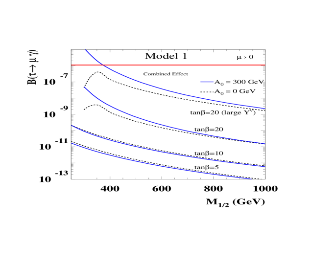
We find that the gaugino contribution to the Ο„β†’ΞΌβ€‹Ξ³β†’πœπœ‡π›Ύ\tau\rightarrow\mu\gamma decay rate is always suppressed since Ο„Lsubscript𝜏𝐿\tau_{L} and ΞΌLsubscriptπœ‡πΏ\mu_{L} have the same flavor charges and since the Ο„Rsubscriptπœπ‘…\tau_{R}–μRsubscriptπœ‡π‘…\mu_{R} mixing angle is of order Ο΅2superscriptitalic-Ο΅2\epsilon^{2}. The only significant effect to this process is from the right–handed neutrino effects when p=0𝑝0p=0.

4.2 Numerical Results

In this section we present our numerical results for the LFV processes ΞΌβ†’eβ€‹Ξ³β†’πœ‡π‘’π›Ύ\mu\rightarrow e\gamma and Ο„β†’ΞΌβ€‹Ξ³β†’πœπœ‡π›Ύ\tau\rightarrow\mu\gamma. We adopt the mSUGRA scenario for the SUSY breaking parameters. At the string scale, taken to be Ms​t=1017subscript𝑀𝑠𝑑superscript1017M_{st}=10^{17} GeV, we assume a universal scalar mass m0subscriptπ‘š0m_{0} and a common gaugino soft masses M1/2subscript𝑀12M_{1/2}. The unified gauge coupling at 2Γ—10162superscript10162\times 10^{16} GeV is taken to be Ξ±G≃1/24similar-to-or-equalssubscript𝛼𝐺124\alpha_{G}\simeq 1/24. We assume the U​(1)Aπ‘ˆsubscript1𝐴U(1)_{A} gauge coupling gFsubscript𝑔𝐹g_{F} to be equal to g2subscript𝑔2g_{2} at the string scale. We evolve the soft SUSY breaking parameters from Ms​tsubscript𝑀𝑠𝑑M_{st} to the U​(1)Aπ‘ˆsubscript1𝐴U(1)_{A} gaugino mass MF≃Ms​t/80similar-to-or-equalssubscript𝑀𝐹subscript𝑀𝑠𝑑80M_{F}\simeq M_{st}/80 (see Eqs. (15) and (16)). We use the numerical values of the Yukawa couplings given in Eqs. (27)-(2.3) for this evolution.

As explained previously, we take m0=M1/2/4.4subscriptπ‘š0subscript𝑀124.4m_{0}=M_{1/2}/4.4 so that the relic abundance of neutralino dark matter can be reproduced correctly. With this choice we always find the neutralino to be the LSP with the Ο„~Rsubscript~πœπ‘…\tilde{\tau}_{R} mass higher than the LSP mass by 5βˆ’155155-15 GeV. We impose radiative electroweak symmetry breaking condition. The SUSY higgs mass parameter ΞΌπœ‡\mu is chosen to be positive which is favored by bβ†’s​γ→𝑏𝑠𝛾b\rightarrow s\gamma.

We take M1/2subscript𝑀12M_{1/2} to vary in the range 250250250 GeV to 111 TeV. The lower value satisfies the lightest higgs boson mass limit. We present the results for three different values of tan⁑β=(5, 10, 20)𝛽51020\tan\beta=(5,\,10,\,20). The corresponding values of the exponent p𝑝p are taken to be p=(2, 1, 0)𝑝21 0p=(2,\,1,\,0). The results are presented for two different values of A0=(0, 300)subscript𝐴00300A_{0}=(0,\,300) GeV. When tan⁑β=20𝛽20\tan\beta=20, the lower limit on M1/2subscript𝑀12M_{1/2} is around 300300300 GeV, or else the radiative electroweak symmetry breaking would fail. The branching ratios are plotted against universal gaugino mass M1/2subscript𝑀12M_{1/2} in Figures 3–14.

In Figure 3, we plot the branching ratio for the process ΞΌβ†’eβ€‹Ξ³β†’πœ‡π‘’π›Ύ\mu\rightarrow e\gamma including all the LFV effects described earlier for Model 1 as a function of M1/2subscript𝑀12M_{1/2} for different values of tan⁑β𝛽\tan\beta and A0subscript𝐴0A_{0}. We see that the branching ratio is in the experimentally interesting range for most of the parameter space. In this Figure for tan⁑β=20𝛽20\tan\beta=20 we also show the branching ratio when the Dirac neutrino Yukawa coupling effects are maximized (denoted by β€œlarge YΞ½superscriptπ‘ŒπœˆY^{\nu}”). The horizontal line corresponds to the current experimental limit.

In Figure 4 the combined effect for ΞΌβ†’eβ€‹Ξ³β†’πœ‡π‘’π›Ύ\mu\rightarrow e\gamma is plotted for Model 2.

In Figure 5 we plot B​(ΞΌβ†’e​γ)π΅β†’πœ‡π‘’π›ΎB\left(\mu\rightarrow e\gamma\right) induced solely by the right–handed neutrino Yukawa couplings. This result is identical for Models 1 and 2 since neutrino textures are the same for the two models. In Figure 6 we plot the branching ratio induced by the right–handed neutrino effects and the flavor gaugino effects for Model 1. Figure 7 has the same plot for Model 2. In Figure 8 (9) we plot B​(ΞΌβ†’e​γ)π΅β†’πœ‡π‘’π›ΎB\left(\mu\rightarrow e\gamma\right) induced by the trace term and the right–handed neutrino for Model 1 (2). Figure 10 (11) is a plot of the branching ratio including the effects of A𝐴A–terms and Ξ½csuperscriptπœˆπ‘\nu^{c} for Model 1 (2). Figures 12 and 13 are the branching ratios for Ο„β†’ΞΌβ€‹Ξ³β†’πœπœ‡π›Ύ\tau\rightarrow\mu\gamma including all LFV effects for Model 1 and Model 2. Figure 14, which is valid for both Models 1 and 2, has the branching ratios for Ο„β†’ΞΌβ€‹Ξ³β†’πœπœ‡π›Ύ\tau\rightarrow\mu\gamma induced only by the Ξ½csuperscriptπœˆπ‘\nu^{c} Yukawa coupling effects.

From these figures we see that the decay ΞΌβ†’eβ€‹Ξ³β†’πœ‡π‘’π›Ύ\mu\rightarrow e\gamma is within the reach of forthcoming experiments. Discovery of Ο„β†’ΞΌβ€‹Ξ³β†’πœπœ‡π›Ύ\tau\rightarrow\mu\gamma decay will strongly hint, within our framework, an origin related to the right–handed neutrino Yukawa couplings.
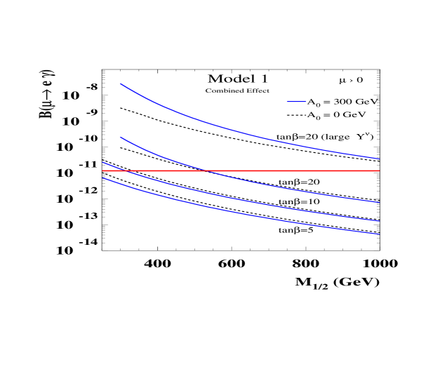
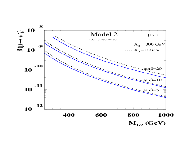
Refer to caption
Figure 3: Branching ratio for the process ΞΌβ†’eβ€‹Ξ³β†’πœ‡π‘’π›Ύ\mu\rightarrow e\gamma including all corrections for Model 1. The solid line corresponds to A0=300subscript𝐴0300A_{0}=300 GeV and the dashed line corresponds to A0=0subscript𝐴00A_{0}=0 GeV. For tan⁑β=20𝛽20\tan\beta=20 we give two sets of curves, the upper one corresponds to the maximal value of the neutrino Yukawa coupling YΞ½superscriptπ‘ŒπœˆY^{\nu}. Here and in other plots, the straight horizontal line corresponds to the current experimental limit B​(ΞΌβ†’e​γ)e​x​p<1.2Γ—10βˆ’11𝐡subscriptβ†’πœ‡π‘’π›Ύπ‘’π‘₯𝑝1.2superscript1011B(\mu\rightarrow e\gamma)_{exp}<1.2\times 10^{-11} [24].
Refer to caption
Figure 4: Branching ratio for the process ΞΌβ†’eβ€‹Ξ³β†’πœ‡π‘’π›Ύ\mu\rightarrow e\gamma including all corrections for Model 2.
Refer to caption
Figure 5: Branching ratio for the process ΞΌβ†’eβ€‹Ξ³β†’πœ‡π‘’π›Ύ\mu\rightarrow e\gamma induced by only the right–handed neutrino Yukawa coupling effects. This result holds for both Models 1 and 2.
Refer to caption
Figure 6: Branching ratio for the process ΞΌβ†’eβ€‹Ξ³β†’πœ‡π‘’π›Ύ\mu\rightarrow e\gamma induced by the gaugino corrections (plus Ξ½csuperscriptπœˆπ‘\nu^{c} effects) for Model 1.
Refer to caption
Figure 7: Branching ratio for the process ΞΌβ†’eβ€‹Ξ³β†’πœ‡π‘’π›Ύ\mu\rightarrow e\gamma induced by the gaugino corrections (plus Ξ½csuperscriptπœˆπ‘\nu^{c} effects) for Model 2.
Refer to caption
Figure 8: Branching ratio for the process ΞΌβ†’eβ€‹Ξ³β†’πœ‡π‘’π›Ύ\mu\rightarrow e\gamma induced by the trace correction (plus Ξ½csuperscriptπœˆπ‘\nu^{c} effects) for Model 1.
Refer to caption
Figure 9: Branching ratio for the process ΞΌβ†’eβ€‹Ξ³β†’πœ‡π‘’π›Ύ\mu\rightarrow e\gamma induced by the trace correction (plus Ξ½csuperscriptπœˆπ‘\nu^{c} effects) for Model 2.
Refer to caption
Figure 10: Branching ratio for the process ΞΌβ†’eβ€‹Ξ³β†’πœ‡π‘’π›Ύ\mu\rightarrow e\gamma from the vertex corrections (plus Ξ½csuperscriptπœˆπ‘\nu^{c} effects) for Model 1.
Refer to caption
Figure 11: Branching ratio for the process ΞΌβ†’eβ€‹Ξ³β†’πœ‡π‘’π›Ύ\mu\rightarrow e\gamma from the vertex corrections (plus Ξ½csuperscriptπœˆπ‘\nu^{c} effects) for Model 2.
Refer to caption
Figure 12: Branching ratio for the process Ο„β†’ΞΌβ€‹Ξ³β†’πœπœ‡π›Ύ\tau\rightarrow\mu\gamma including all the effects for Model 1.
Refer to caption
Figure 13: Branching ratio for the process Ο„β†’ΞΌβ€‹Ξ³β†’πœπœ‡π›Ύ\tau\rightarrow\mu\gamma including all the effects for Model 2.
Refer to caption
Figure 14: Branching ratio for the process Ο„β†’ΞΌβ€‹Ξ³β†’πœπœ‡π›Ύ\tau\rightarrow\mu\gamma induced by only the right–handed neutrino Yukawa coupling effects for Models 1 and 2.

4.3 The D–term Splitting Problem

Any model based on a gauged flavor symmetry has a potential D𝐷D–term splitting problem, which could give rise to large FCNC processes even with a universal choice of soft scalar masses. Here we quantify this problem in the class of anomalous U​(1)π‘ˆ1U(1) models. We point out that this problem is not as serious as it might naively appear, if the hierarchy m0=M1/2/4.4subscriptπ‘š0subscript𝑀124.4m_{0}=M_{1/2}/4.4 needed for an acceptable relic abundance of neutralino dark matter is assumed.

The DAsubscript𝐷𝐴D_{A}–term contribution to the scalar potential including soft SUSY breaking mass for the flavon field S𝑆S is given by

V=m~s2​|S|2+|qs|2​gF28​(ΞΎ|qs|βˆ’|S|2+βˆ‘iqi​|f~i|2)2𝑉subscriptsuperscript~π‘š2𝑠superscript𝑆2superscriptsubscriptπ‘žπ‘ 2superscriptsubscript𝑔𝐹28superscriptπœ‰subscriptπ‘žπ‘ superscript𝑆2subscript𝑖subscriptπ‘žπ‘–superscriptsubscript~𝑓𝑖22\displaystyle V=\tilde{m}^{2}_{s}|S|^{2}+\frac{|q_{s}|^{2}g_{F}^{2}}{8}\left(\frac{\xi}{|q_{s}|}-|S|^{2}+\sum_{i}q_{i}|\tilde{f}_{i}|^{2}\right)^{2} (58)

where qssubscriptπ‘žπ‘ q_{s} and qisubscriptπ‘žπ‘–q_{i} are the U​(1)Aπ‘ˆsubscript1𝐴U(1)_{A} flavor charges of the S𝑆S field and the MSSM fields f~isubscript~𝑓𝑖\tilde{f}_{i}. Minimizing the potential one finds the mass splitting among the MSSM sfermions to be

m~fi2βˆ’m~fj2=qiβˆ’qj|qs|​m~s2.superscriptsubscript~π‘šsubscript𝑓𝑖2superscriptsubscript~π‘šsubscript𝑓𝑗2subscriptπ‘žπ‘–subscriptπ‘žπ‘—subscriptπ‘žπ‘ superscriptsubscript~π‘šπ‘ 2\displaystyle\tilde{m}_{f_{i}}^{2}-\tilde{m}_{f_{j}}^{2}=\frac{q_{i}-q_{j}}{|q_{s}|}\tilde{m}_{s}^{2}. (59)

If a universal scalar mass is assumed even for m~s2subscriptsuperscript~π‘š2𝑠\tilde{m}^{2}_{s}, this splitting could be unacceptably large. However, if we choose m0=M1/2/4.4subscriptπ‘š0subscript𝑀124.4m_{0}=M_{1/2}/4.4, this may be in an acceptable range. The low energy values for the slepton soft masses including the DAsubscript𝐷𝐴D_{A}–term corrections to Eq. (4.1) are

(m~L2)i​i=qiL|qs|​m~s2+m02+0.52​M1/22≃qiL|qs|​m~s2+11.1​m02,subscriptsuperscriptsubscript~π‘šπΏ2𝑖𝑖subscriptsuperscriptπ‘žπΏπ‘–subscriptπ‘žπ‘ subscriptsuperscript~π‘š2𝑠superscriptsubscriptπ‘š020.52superscriptsubscript𝑀122similar-to-or-equalssubscriptsuperscriptπ‘žπΏπ‘–subscriptπ‘žπ‘ subscriptsuperscript~π‘š2𝑠11.1superscriptsubscriptπ‘š02\displaystyle\left(\tilde{m}_{L}^{2}\right)_{ii}=\frac{q^{L}_{i}}{|q_{s}|}\tilde{m}^{2}_{s}+m_{0}^{2}+0.52\,M_{1/2}^{2}\simeq\frac{q^{L}_{i}}{|q_{s}|}\tilde{m}^{2}_{s}+11.1\,m_{0}^{2}\,,
(m~e2)i​i=qie|qs|​m~s2+m02+0.15​M1/22≃qie|qs|​m~s2+3.9​m02.subscriptsuperscriptsubscript~π‘šπ‘’2𝑖𝑖subscriptsuperscriptπ‘žπ‘’π‘–subscriptπ‘žπ‘ subscriptsuperscript~π‘š2𝑠superscriptsubscriptπ‘š020.15superscriptsubscript𝑀122similar-to-or-equalssubscriptsuperscriptπ‘žπ‘’π‘–subscriptπ‘žπ‘ subscriptsuperscript~π‘š2𝑠3.9superscriptsubscriptπ‘š02\displaystyle\left(\tilde{m}_{e}^{2}\right)_{ii}=\frac{q^{e}_{i}}{|q_{s}|}\tilde{m}^{2}_{s}+m_{0}^{2}+0.15\,M_{1/2}^{2}\simeq\frac{q^{e}_{i}}{|q_{s}|}\tilde{m}^{2}_{s}+3.9\,m_{0}^{2}\,. (60)

Since the D𝐷D–terms only contribute to the diagonal slepton mass splittings, any flavor violation arising from it must involve fermionic mixing angles. We find

(Ξ΄R​R)12esubscriptsuperscriptsuperscript𝛿𝑅𝑅𝑒12\displaystyle\left(\delta^{RR}\right)^{e}_{12} ≃similar-to-or-equals\displaystyle\simeq δ​q12e​Y21e​m~s2Y22e​(m~e2)22,𝛿subscriptsuperscriptπ‘žπ‘’12subscriptsuperscriptπ‘Œπ‘’21superscriptsubscript~π‘šπ‘ 2subscriptsuperscriptπ‘Œπ‘’22subscriptsuperscriptsubscript~π‘šπ‘’222\displaystyle\frac{\delta q^{e}_{12}Y^{e}_{21}\tilde{m}_{s}^{2}}{Y^{e}_{22}\left(\tilde{m}_{e}^{2}\right)_{22}}\,, (61)
(Ξ΄L​L)12esubscriptsuperscriptsuperscript𝛿𝐿𝐿𝑒12\displaystyle\left(\delta^{LL}\right)^{e}_{12} ≃similar-to-or-equals\displaystyle\simeq δ​q12L​Y12e​m~s2Y22e​(m~L2)22,𝛿subscriptsuperscriptπ‘žπΏ12subscriptsuperscriptπ‘Œπ‘’12superscriptsubscript~π‘šπ‘ 2subscriptsuperscriptπ‘Œπ‘’22subscriptsuperscriptsubscript~π‘šπΏ222\displaystyle\frac{\delta q^{L}_{12}Y^{e}_{12}\,\tilde{m}_{s}^{2}}{Y^{e}_{22}\left(\tilde{m}_{L}^{2}\right)_{22}}\,, (62)

where (Ξ΄R​R)12esubscriptsuperscriptsuperscript𝛿𝑅𝑅𝑒12\left(\delta^{RR}\right)^{e}_{12} is the e~Rsubscript~𝑒𝑅\tilde{e}_{R}–μ~Rsubscript~πœ‡π‘…\tilde{\mu}_{R} mixing parameter in the supersymmetric basis. Here δ​q12e=(q1eβˆ’q2e)/|qs|=2βˆ’Ξ±π›Ώsubscriptsuperscriptπ‘žπ‘’12subscriptsuperscriptπ‘žπ‘’1subscriptsuperscriptπ‘žπ‘’2subscriptπ‘žπ‘ 2𝛼\delta q^{e}_{12}=(q^{e}_{1}-q^{e}_{2})/|q_{s}|=2-\alpha and δ​q12L=(q1Lβˆ’q2L)/|qs|=1𝛿subscriptsuperscriptπ‘žπΏ12subscriptsuperscriptπ‘žπΏ1subscriptsuperscriptπ‘žπΏ2subscriptπ‘žπ‘ 1\delta q^{L}_{12}=(q^{L}_{1}-q^{L}_{2})/|q_{s}|=1, with Ξ±=0​(1)𝛼01\alpha=0\,(1) for Model 1 (Model 2). For ΞΌβ†’eβ€‹Ξ³β†’πœ‡π‘’π›Ύ\mu\rightarrow e\gamma this gives

(Ξ΄R​R)12esubscriptsuperscriptsuperscript𝛿𝑅𝑅𝑒12\displaystyle\left(\delta^{RR}\right)^{e}_{12} ≃similar-to-or-equals\displaystyle\simeq CR​(2βˆ’Ξ±)​ϡ1βˆ’Ξ±β€‹(m~sm0)21+11.95​(m~sm0)2,subscript𝐢𝑅2𝛼superscriptitalic-Ο΅1𝛼superscriptsubscript~π‘šπ‘ subscriptπ‘š02111.95superscriptsubscript~π‘šπ‘ subscriptπ‘š02\displaystyle C_{R}\,\frac{(2-\alpha)\epsilon^{1-\alpha}\left(\frac{\tilde{m}_{s}}{m_{0}}\right)^{2}}{1+\frac{1}{1.95}\left(\frac{\tilde{m}_{s}}{m_{0}}\right)^{2}}\,, (63)
(Ξ΄L​L)12esubscriptsuperscriptsuperscript𝛿𝐿𝐿𝑒12\displaystyle\left(\delta^{LL}\right)^{e}_{12} ≃similar-to-or-equals\displaystyle\simeq CL​(m~sm0)21+p11.1​(m~sm0)2,subscript𝐢𝐿superscriptsubscript~π‘šπ‘ subscriptπ‘š021𝑝11.1superscriptsubscript~π‘šπ‘ subscriptπ‘š02\displaystyle C_{L}\,\frac{\left(\frac{\tilde{m}_{s}}{m_{0}}\right)^{2}}{1+\frac{p}{11.1}\left(\frac{\tilde{m}_{s}}{m_{0}}\right)^{2}}\,, (64)

where

CR=ϡ​Y21e3.9​Y22e≃(186.9,146.9),subscript𝐢𝑅italic-Ο΅subscriptsuperscriptπ‘Œπ‘’213.9subscriptsuperscriptπ‘Œπ‘’22similar-to-or-equals186.9146.9\displaystyle C_{R}=\frac{\epsilon\,Y^{e}_{21}}{3.9\,Y^{e}_{22}}\simeq\left(\frac{1}{86.9},\,\frac{1}{46.9}\right),
CL=ϡ​Y12e11.1​Y22e≃(175.6,172.)​for (Model 1, Model 2).\displaystyle C_{L}=\frac{\epsilon\,Y^{e}_{12}}{11.1\,Y^{e}_{22}}\simeq\left(\frac{1}{75.6},\,\frac{1}{72.}\right)\,\,\,\mbox{for (Model 1, Model 2)}. (65)

From the experimental bound on ΞΌβ†’eβ€‹Ξ³β†’πœ‡π‘’π›Ύ\mu\rightarrow e\gamma one approximately has [8]

(Ξ΄L​L)12e|β‰ˆe​x​p(Ξ΄R​R)12e|e​x​p< 1.2Γ—10βˆ’21tan⁑β(MS​U​S​Y500​GeV)2.\displaystyle\left(\delta^{LL}\right)^{e}_{12}\left|{}_{exp}\approx\left(\delta^{RR}\right)^{e}_{12}\right|_{exp}<\,1.2\times 10^{-2}\frac{1}{\tan\beta}\left(\frac{M_{SUSY}}{500\,\mbox{GeV}}\right)^{2}. (66)

For tan⁑β=5𝛽5\tan\beta=5 and for MS​U​S​Y≃M1/2similar-to-or-equalssubscriptπ‘€π‘†π‘ˆπ‘†π‘Œsubscript𝑀12M_{SUSY}\simeq M_{1/2} (which is a reasonable choice) we find

(Ξ΄L​L,R​R)12e|<e​x​p0.6Γ—10βˆ’3(1.0Γ—10βˆ’2)forM1/2=250(1000)GeV.\displaystyle\left(\delta^{LL,RR}\right)^{e}_{12}\left|{}_{exp}<0.6\times 10^{-3}\,\left(1.0\times 10^{-2}\right)\right.\,\,\mbox{for}\,\,M_{1/2}=250\,\left(1000\right)\,\mbox{GeV}\,. (67)

This gives the following constraint on m~s/m0subscript~π‘šπ‘ subscriptπ‘š0\tilde{m}_{s}/m_{0}:

m~sm0<0.2​(0.9)​for​M1/2=250​(1000)​GeVsubscript~π‘šπ‘ subscriptπ‘š00.20.9forsubscript𝑀122501000GeV\displaystyle\frac{\tilde{m}_{s}}{m_{0}}<0.2\,\left(0.9\right)\,\,\mbox{for}\,\,M_{1/2}=250\,\left(1000\right)\,\mbox{GeV}\, (68)

for Model 1 and

m~sm0<0.17​(0.7)​for​M1/2=250​(1000)​GeVsubscript~π‘šπ‘ subscriptπ‘š00.170.7forsubscript𝑀122501000GeV\displaystyle\frac{\tilde{m}_{s}}{m_{0}}<0.17\,\left(0.7\right)\,\,\mbox{for}\,\,M_{1/2}=250\,\left(1000\right)\,\mbox{GeV}\, (69)

for Model 2. For low values of M1/2subscript𝑀12M_{1/2} this gives a significant constraint on m~ssubscript~π‘šπ‘ \tilde{m}_{s}, while for large values of M1/2subscript𝑀12M_{1/2} universality of all scalar masses may be maintained.

We wish to note that the m~s2superscriptsubscript~π‘šπ‘ 2\tilde{m}_{s}^{2} appearing in Eq. (59) and in the subsequent discussions is the soft mass–squared of the scalar flavon field S𝑆S evaluated at the U​(1)Aπ‘ˆsubscript1𝐴U(1)_{A} breaking scale MFsubscript𝑀𝐹M_{F}. Since there are singlet fields Xksubscriptπ‘‹π‘˜X_{k} in the theory needed for anomaly cancellation which are active between the U​(1)Aπ‘ˆsubscript1𝐴U(1)_{A} scale and Ms​tsubscript𝑀𝑠𝑑M_{st} (Cf: Eq. (9)), the S𝑆S field can have renormalizable Yukawa couplings of the type Yk​Xk​Xk¯​Ssubscriptπ‘Œπ‘˜subscriptπ‘‹π‘˜Β―subscriptπ‘‹π‘˜π‘†Y_{k}X_{k}\bar{X_{k}}S where XkΒ―Β―subscriptπ‘‹π‘˜\bar{X_{k}} are fields neutral under U​(1)Aπ‘ˆsubscript1𝐴U(1)_{A}. We have examined the evolution of m~s2superscriptsubscript~π‘šπ‘ 2\tilde{m}_{s}^{2} between MFsubscript𝑀𝐹M_{F} and Ms​tsubscript𝑀𝑠𝑑M_{st} in the presence of such Yukawa couplings and found that even with the limits on m~ssubscript~π‘šπ‘ \tilde{m}_{s} given in Eqs. (68) and (69), m~s2=m02superscriptsubscript~π‘šπ‘ 2superscriptsubscriptπ‘š02\tilde{m}_{s}^{2}=m_{0}^{2} can be attained at the string scale for a range of Yukawa couplings Yksubscriptπ‘Œπ‘˜Y_{k}.

The RGE running of m~s2superscriptsubscript~π‘šπ‘ 2\tilde{m}_{s}^{2} between the string scale and the U​(1)Aπ‘ˆsubscript1𝐴U(1)_{A} symmetry breaking scale contains the same trace term and the same gaugino contributions that we considered for the MSSM sfermions in Eqs. (4.1) and (4.1) (see also terms proportional to ΟƒπœŽ\sigma in Eqs. (36)-(41))

Ξ΄m~s2β‰ƒβˆ’qs|qs|gF2(3m02βˆ‘i=1,3(ni​iu+ni​id)\displaystyle\delta\tilde{m}_{s}^{2}\simeq-q_{s}|q_{s}|g_{F}^{2}\left(3\,m_{0}^{2}\,\sum_{i=1,3}\left(n^{u}_{ii}+n^{d}_{ii}\right)\right.
+m02βˆ‘i=1,3(ni​ie+ni​iΞ½)+nXm02βˆ’m~s2)ln​(Ms​t/MF)8​π2\displaystyle\,\,\,\,\,\,\,\left.+m_{0}^{2}\,\sum_{i=1,3}\left(n^{e}_{ii}+n^{\nu}_{ii}\right)+n^{X}m_{0}^{2}-\tilde{m}_{s}^{2}\right)\frac{{\rm ln}\left(M_{st}/M_{F}\right)}{8\pi^{2}}
+(qs​gF)2​(MΞ»F)2​ln​(Ms​t/MF)2​π2.superscriptsubscriptπ‘žπ‘ subscript𝑔𝐹2superscriptsubscript𝑀subscriptπœ†πΉ2lnsubscript𝑀𝑠𝑑subscript𝑀𝐹2superscriptπœ‹2\displaystyle\,\,\,\,\,\,\,+\left(q_{s}\,g_{F}\right)^{2}\left(M_{\lambda_{F}}\right)^{2}\frac{{\rm ln}\left(M_{st}/M_{F}\right)}{2\pi^{2}}\,. (70)

Interestingly, this contribution from the D𝐷D-term evolution cancels the β€œtrace contributions” in the sfermion masses (the terms proportional to ΟƒπœŽ\sigma in Eqs. (36)-(41)) [25].

5 Conclusion

In this paper we have studied lepton flavor violation induced by a flavor–dependent anomalous U​(1)π‘ˆ1U(1) gauge symmetry of string origin in a class of models which addresses the fermion mass hierarchy problem via the Froggatt–Nielsen mechanism. We have derived a general set of renormalization group equations for the evolution of soft SUSY breaking parameters in the presence of higher dimensional operators. These results should be applicable to a large class of fermion mass models. We have shown that the U​(1)Aπ‘ˆsubscript1𝐴U(1)_{A} sector induces significant flavor violation in the SUSY breaking parameters during the RGE evolution from the string scale to the flavor symmetry breaking scale, even though this momentum range is very short. We have identified several sources of flavor violation: the U​(1)Aπ‘ˆsubscript1𝐴U(1)_{A} gaugino contribution to the scalar masses which is flavor dependent, a contribution proportional to the trace of U​(1)Aπ‘ˆsubscript1𝐴U(1)_{A} charge which is also flavor dependent, non–proportional A𝐴A–terms arising from the U​(1)Aπ‘ˆsubscript1𝐴U(1)_{A} gaugino vertex correction diagrams, and the U​(1)Aπ‘ˆsubscript1𝐴U(1)_{A} D𝐷D–term. In addition, there are flavor violating effects in the charged lepton sector arising from the right–handed neutrino Yukawa couplings, which have also been included in our numerical analysis. The resulting flavor violation in the leptonic decays ΞΌβ†’eβ€‹Ξ³β†’πœ‡π‘’π›Ύ\mu\rightarrow e\gamma and Ο„β†’ΞΌβ€‹Ξ³β†’πœπœ‡π›Ύ\tau\rightarrow\mu\gamma are found to be in the experimentally interesting range.

Adopting the minimal supergravity scenario for SUSY breaking, and choosing parameters such that the needed relic abundance of neutralino dark matter is realized, we have presented results for the branching ratios B​(ΞΌβ†’e​γ)π΅β†’πœ‡π‘’π›ΎB(\mu\rightarrow e\gamma) and B​(τ→μ​γ)π΅β†’πœπœ‡π›ΎB(\tau\rightarrow\mu\gamma) in two specific models of fermion masses. Figures 3 and 4 are our main results for the two models for B​(ΞΌβ†’e​γ)π΅β†’πœ‡π‘’π›ΎB(\mu\rightarrow e\gamma), while Figures 13 and 14 are our results for B​(τ→μ​γ)π΅β†’πœπœ‡π›ΎB(\tau\rightarrow\mu\gamma). The former should be accessible to forthcoming experiments, while the latter is also in the observable range. Although we focused on two specific fermion mass textures these effects should be significant in a large class of models.

Acknowledgments

We thank C. Macesanu for helpful discussions. This work is supported in part by DOE Grant # DE-FG03-98ER-41076, an award from the Research Corporation and by DOE Grant # DE-FG02-01ER-45684.

References

  • [1] C.D. Froggatt and H.B. Nielsen, Nucl. Phys. B147, 277 (1979).
  • [2] M.B. Green and J.H. Schwarz, Phys. Lett. B149, 117 (1984); M.B. Green and J.H. Schwarz, Nucl. Phys. B255, 93 (1985); M.B. Green, J.H. Schwarz and P. West, Nucl. Phys. B254, 327 (1985).
  • [3] M. Dine, N. Seiberg and E. Witten, Nucl. Phys. B289, 589 (1987); J. Atick, L. Dixon and A. Sen, Nucl. Phys. B292, 109 (1987).
  • [4] L. E. Ibanez, G. G. Ross, Phys. Lett. B332, 100 (1994); E. Dudas, S. Pokorski and C.A. Savoy, Phys. Lett. B356, 45 (1995); P. Binetruy and P. Ramond, Phys. Lett. B350, 49 (1995); Y. Nir, Phys. Lett. B354, 107 (1995); E. J. Chun, A. Lukas, Phys. Lett. B387, 99 (1996); P. Binetruy, S. Lavignac and P. Ramond, Nucl. Phys. B477, 353 (1996); Y. Nir and R. Rattazzi, Phys. Lett. B382, 363 (1996); A. H. Chamseddine and H. K. Dreiner, Phys. Lett. B389, 533 (1996); P. Binetruy, S. Lavignac, S.T. Petcov and P. Ramond, Nucl. Phys. B496, 3 (1997); K. Choi, E. J. Chun and H. D. Kim, Phys. Lett. B394, 89 (1997); Z. Berezhiani and Z. Tavartkiladze, Phys. Lett. B396, 150 (1997), Phys. Lett. B409, 220 (1997); P. Binetruy, E. Dudas, S. Lavignac and C.A. Savoy, Phys. Lett. B422, 171 (1998); J. K. Elwood, N. Irges and P. Ramond, Phys. Rev. Lett. 81, 5064 (1998); Y Grossman, Y. Nir and Y. Shadmi, JHEP 9810, 007 (1998); G. Altarelli and F. Feruglio, JHEP 9811, 021 (1998), Phys. Rept. 320, 295 (1999); Q. Shafi and Z. Tavartkiladze, Phys. Lett. B451, 129 (1999), Phys. Lett. B482, 145 (2000); G. Eyal, Phys. Lett. B461, 71 (1999); M. E. Gomez, G. K. Leontaris, S. Lola and J. D. Vergados, Phys. Rev. D59, 116009 (1999); K. Choi, K. Hwang and E. J. Chun, Phys. Rev. D60, 031301 (1999); J. Feng and Y. Nir, Phys. Rev. D61, 113005 (2000); A.S. Joshipura, R. Vaidya and S.K. Vempati, Phys. Rev. D62, 093020 (2000); M.S. Berger, K. Siyeon, Phys. Rev. D62, 033004 (2000), Phys. Rev. D64, 053006 (2001); N. Maekawa, Prog. Theor. Phys. 106, 401 (2001); J. Sato and K. Tobe, Phys. Rev. D63, 116010 (2001); M. Tanimoto, Phys. Lett. B501, 231 (2001); I. Gogoladze and A. Perez-Lorenzana, Phys. Rev. D65, 095011 (2002); I. Jack, D.R.T. Jones and R. Wild, Phys. Lett. B535, 193 (2002); T. Ohlsson and G. Seidl, Nucl. Phys. B643, 247 (2002); S.M. Barr and I. Dorsner, Phys. Rev. D65, 095004 (2002); H.K. Dreiner, M. Thormeier, hep-ph/0305270.
  • [5] K.S. Babu, I. Gogoladze and K. Wang, Nucl. Phys. B660, 322 (2003).
  • [6] Y. Kawamura, H. Murayama and M. Yamaguchi, Phys. Rev. D51, 1337 (1995); C. Kolda and S.P. Martin, Phys. Rev. D53, 3871 (1996).
  • [7] K.S. Babu and S.M. Barr, Phys. Lett. B387, 87 (1996); K.S. Babu and R.N. Mohapatra, Phys. Rev. Lett. 83, 2522 (1999).
  • [8] B. Murakami, K. Tobe and J.D. Wells, Phys. Lett. B526, 157 (2002).
  • [9] F. Borzumati and A. Masiero, Phys. Rev. Lett. 57, 961 (1986); J. Hisano, T. Moroi, K. Tobe, M. Yamaguchi and T. Yanagida, Phys. Lett. B357, 579 (1995); J. Hisano, T. Moroi, K. Tobe and M. Yamaguchi, Phys. Rev. D53, 2442 (1996).
  • [10] S.F. King and M. Oliveira, Phys. Rev. D60, 035003 (1999); J. Hisano and D. Nomura, Phys. Rev. D59, 116005 (1999); K.S. Babu, B. Dutta and R.N. Mohapatra, Phys. Lett. B458, 93 (1999); W. Buchmuller, D. Delepine and F. Vissani, Phys. Lett. B459, 171 (1999); J. Ellis, M. Gomez, G. Leontaris, S. Lola and D. Nanopoulos, Eur. Phys. J. C14, 319 (2000); S. Lavignac, I. Masina and C. Savoy, Phys. Lett. B520, 269 (2001); Nucl. Phys. B633, 139 (2002); J. Casas and A. Ibarra, Nucl. Phys. B618, 171 (2001); R. Gonzalez Felipe and F. Joaquim, JHEP 0109, 015 (2001); J. Sato, K. Tobe and T. Yanagida, Phys. Lett. B498, 189 (2001); X.J. Bi, Y.B. Dai and X.Y. Qi, Phys. Rev. D63, 096008 (2001), Phys. Rev. D66, 076006 (2002); G. Cvetic, C. Dib, C.S. Kim and J.D. Kim, Phys. Rev. D66, 034008 (2002); J. Ellis, J. Hisano, S. Lola and M. Raidal, Nucl. Phys. B621, 208 (2002); A. Kageyama, S. Kaneko, N. Shimoyama and M. Tanimoto, Phys. Lett. B527, 206 (2002); D. Chang, A. Masiero and H. Murayama, Phys. Rev. D67, 075013 (2003); J. Ellis, J. Hisano, M. Raidal and Y. Shimizu, Phys. Rev. D66, 115013 (2002); K.S. Babu and C. Kolda, Phys. Rev. Lett. 89, 241802 (2002); A. Rossi, Phys. Rev. D66, 075003 (2002); A. Masiero, S.K. Vempati and O. Vives, Nucl. Phys. B649, 189 (2003); B. Dutta, R.N. Mohapatra, hep-ph/0305059.
  • [11] K.S. Babu, B. Dutta and R.N. Mohapatra, Phys. Rev. D67, 076006 (2003).
  • [12] M. Fukugita and T. Yanagida, Phys. Lett. B174, 45 (1986); For a review see W. Buchmuller and M. Plumacher, Int. J. Mod. Phys. A15, 5047 (2000).
  • [13] L.J. Hall, V. Kostelecky and S. Raby, Nucl. Phys. B267, 415, (1986); F. Gabbiani and A. Masiero, Nucl. Phys. B322, 235 (1989); R. Barbieri and L. J. Hall, Phys. Lett. B338, 212 (1994); X.J. Bi, Eur. Phys. J. C27, 399 (2003); S.M. Barr, hep-ph/0307372.
  • [14] K.S. Babu and S.M. Barr, Phys. Lett. B381, 202 (1996).
  • [15] C.H. Albright, K.S. Babu, and S.M. Barr, Phys. Rev. Lett. 81, 1167 (1998); J. Sato and T. Yanagida, Phys. Lett. B430, 127 (1998); N. Irges, S. Lavignac, and P. Ramond, Phys. Rev. D58, 035003 (1998).
  • [16] P. Ginsparg, Phys. Lett. B197, 139 (1987); V. S. Kaplunovsky, Nucl. Phys. B307, 145 (1988).
  • [17] E. Witten, Nucl. Phys. B471, 135 (1996).
  • [18] See for example J. Gasser and H. Leutwyler, Phys. Rept. 87, 77 (1982).
  • [19] E. W. Kolb, M. S. Turner, The early universe, Redwood City, USA: Addison-Wesley (1990), (Frontiers in physics, 69); A. Pilaftsis, Int. J. Mod. Phys. A14, 1811 (1999); E. A. Paschos and M. Flanz, Phys. Rev. D58, 113009 (1998); H.B. Nielsen and Y. Takanishi, Phys. Lett. B507, 241 (2001).
  • [20] S.P. Martin and M.T. Vaughn, Phys. Rev. D50, 2282 (1994).
  • [21] S.P. Martin, Phys. Rev. D61, 035004 (2000).
  • [22] J. Ellis, T. Falk, K. Olive and M. Srednicki, Astropart. Phys. 13, 181 (2000); R. Arnowitt, B. Dutta and Y. Santoso, Nucl. Phys. B606, 59 (2001); J. Ellis, T. Falk, G. Ganis, K. Olive and M. Srednicki, Phys. Lett. B570 236 (2001); M. Gomez, G. Lazarides and C. Pallis, Phys. Rev. D61, 123512 (2000); Phys. Lett. B487, 313 (2000); M. Gomez and J. Vergados, Phys. Lett. B512, 252 (2001); L. Roszkowski, R. Austri and T. Nihei, JHEP 0108, 024 (2001); A. Lahanas, D. Nanopoulos and V. Spanos, Phys. Lett. B518, 94 (2001); J.R. Ellis, K. A. Olive, Y. Santoso and V. C. Spanos, Phys. Lett. B565, 176 (2003); M. Battaglia, A. De Roeck, J. Ellis, F. Gianotti, K.A. Olive and L. Pape, hep-ph/0306219; U. Chattopadhyay, A. Corsetti and P. Nath, hep-ph/0303201.
  • [23] See for example: L.E. Ibanez and C. Lopez, Nucl. Phys. B233, 511 (1984); M. Carena, M. Olechowski, S. Pokorski and C.E.M. Wagner, Nucl. Phys. B426, 269 (1994); W. de Boer, R. Ehret and D.I. Kazakov, Z. Phys. C67, 647 (1995).
  • [24] K.Β Hagiwara et al. [Particle Data Group Collaboration], Phys. Rev. D66, 010001 (2002).
  • [25] T. Kobayashi, H. Nakano, H. Terao and K. Yoshioka, hep-ph/0211347.