Abstract

Exclusive photoproduction of all vector mesons by real and virtual photons is considered in the Soft Dipole Pomeron model. It is emphasized that being the Pomeron in this model a double Regge pole with intercept equal to one, we are led to rising cross-sections but the unitarity bounds are not violated. It is shown that all available data for $\rho,\omega,\varphi,J/\psi$ and $\Upsilon$ in the region of energies 1.7 $\leq W\leq$ 250 GeV and photon virtualities 0 $\leq Q^{2}\leq$ 35 GeV² , including the differential cross-sections in the region of transfer momenta 0 $\leq|t|\leq$ 1.6 GeV², are well described by the model.

1 Introduction

A new precise measurement of $J/\psi$ exclusive photoproduction by ZEUS [1] opens a new window in our understanding of the process and allows us to give more accurate predictions for future experiments.

The key issue of the dataset [1] is the diffractive cone shrinkage observed in $J/\psi$ photoproduction which leads us to consider it a soft rather than pure QCD process so that we can apply the Soft Dipole Pomeron exchange [2] model.

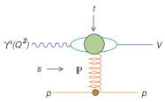
The basic diagram is depicted in Figure 1; $s$ and $t$ are the usual Mandelstam variables, $Q^{2}=-q^{2}$ is the virtuality of the photon.

Figure 1.  : Photoproduction of a vector meson.

It is well known that high-energy representation of the scattering amplitude may be expressed as a sum over the the appropriate Regge poles in the complex $j$ plane [3]

$$A(s,t)_{s\to\infty}\approx\sum\limits_{i}\eta_{i}(t)\beta_{i}(t)(\cos\theta_{t})^{\alpha_{i}(t)},$$ (1)

where $\eta_{i}(t)$ is the signature factor and $\theta_{t}$ is the scattering angle in the $t$ channel.

In the case of vector meson photoproduction we utilize the variable $z\sim\cos\theta_{t}$

$$z=\frac{2(W^{2}-M_{p}^{2})+t+Q^{2}-M_{V}^{2}}{\sqrt{(t+Q^{2}-M_{V}^{2})^{2}+4M_{V}^{2}Q^{2}}}$$ (2)

where $W^{2}=(p+q)^{2}\equiv s$, $M_{V}$ is the vector meson mass, $M_{p}$ is the proton mass.

Assuming vector meson dominance [4], the relation between the forward cross sections of $\gamma p\rightarrow Vp$ and $Vp\rightarrow Vp$ is given by

$$\frac{d\sigma}{dt}(t=0)_{\gamma p\rightarrow Vp}=\frac{4\pi\alpha}{f_{V}^{2}}\frac{d\sigma}{dt}(t=0)_{Vp\rightarrow Vp}$$ (3)

where the strength of the vector meson coupling $\frac{4\pi}{f_{V}^{2}}$ may be found from $e^{+}e^{-}$ decay width of vector meson $V$

$$\Gamma_{V\rightarrow e^{+}e^{-}}=\frac{\alpha^{2}}{3}\frac{4\pi}{f_{V}^{2}}m_{V}$$ (4)

Using the property $\Gamma_{V\rightarrow e^{+}e^{-}}/<Q^{2}_{j}>\simeq const$ we can obtain the following approximate relations

$${m_{\rho}/f_{\rho}^{2}}:{m_{\omega}/f_{\omega}^{2}}:{m_{\varphi}/f_{\varphi}^{2}}:{m_{J/\psi}/f_{J/\psi}^{2}}={9}:{1}:{2}:{8}\;$$ (5)

which are in fairly good agreement with experimental measurements of decay widths [5].

We take into account these relations by introducing coefficients $N_{V}$ (following to [6] ) and writing the amplitude as $A_{\gamma p\rightarrow Vp}=N_{C}N_{V}A_{Vp\rightarrow Vp}$, where

$$N_{C}=3\>;N_{\rho}=\frac{1}{\sqrt{2}}\>;N_{\omega}=\frac{1}{3\sqrt{2}}\>;N_{\phi}=\frac{1}{3}\>;N_{J/\psi}=\frac{2}{3}\>.$$ (6)

The amplitude of the process $Vp\rightarrow Vp$ may be written in the following form

$$A(z,t;M_{V}^{2},\tilde{Q}^{2})={IP}(z,t;M_{V}^{2},\tilde{Q}^{2})+f(z,t;M_{V}^{2},\tilde{Q}^{2})+...\;,$$ (7)

where, $\tilde{Q}^{2}=Q^{2}+M_{V}^{2}$.

${IP}(z,t;M_{V}^{2},\tilde{Q}^{2})$ is the Pomeron contribution for which we use the so called dipole Pomeron which gives a very good description of all hadron-hadron total cross sections [7],[8]. Specifically, ${IP}$ is given by [9]

$${IP}(z,t;M_{V}^{2},\tilde{Q}^{2})=ig_{0}(t;M_{V}^{2},\tilde{Q}^{2})(-iz)^{\alpha_{{IP}}(t)-1}+$$ (8)

$$ig_{1}(t;M_{V}^{2},\tilde{Q}^{2})ln(-iz)(-iz)^{\alpha_{{IP}}(t)-1}\;,$$

where the first term is a single $j$-pole contribution and the second (with an additional $ln(-iz)$ factor) is the contribution of the double $j$-pole.

A similar expression applies to the contribution of the $f$-Reggeon

$$f(z,t;M_{V}^{2},\tilde{Q}^{2})=ig_{f}(t;M_{V}^{2},\tilde{Q}^{2})(-iz)^{\alpha_{f}(t)-1}.$$ (9)

It is important to stress that in this model the intercept of the Pomeron trajectory is equal to 1

$$\alpha_{{IP}}(0)=1.$$ (10)

Thus the model does not violate the Froissart-Martin bound  [10].

For $\rho$ and $\varphi$ meson photoproduction we write the scattering amplitude as the sum of a Pomeron and $f$ contribution. According to the Okubo-Zweig rule, the $f$ meson contribution should be suppressed in the production of the $\varphi$ and $J/\psi$ mesons, but given the present crudeness of the state of the art, we added the $f$ meson contribution in the $\varphi$ meson case.

For $\omega$ meson photoproduction, we include also $\pi$ meson exchange (see also the discussion in [11]), which is needed in the low energy sector given that we try to describe the data for all energies $W$. Even though we did not expect it, the model describes well the data down to threshold.

In the integrated elastic cross section

$$\sigma(z,M_{V}^{2},\tilde{Q}^{2})^{\gamma p\rightarrow Vp}_{el}=4\pi\int\limits_{t_{-}}^{t_{+}}dt|A^{\gamma p\rightarrow Vp}(z,t;M_{V}^{2},\tilde{Q}^{2})|^{2}\;,$$ (11)

the upper and lower limits

$$2t_{\pm}=\pm\frac{L_{1}L_{2}}{W^{2}}-(W^{2}+Q^{2}-M_{V}^{2}-2M_{p}^{2})+\frac{(Q^{2}+M_{p}^{2})(M_{V}^{2}-M_{p}^{2})}{W^{2}},$$ (12)

$$L_{1}=\lambda(W^{2},-Q^{2},M_{p}^{2}),\qquad L_{2}=\lambda(W^{2},M_{V}^{2},M_{p}^{2}),$$ (13)

$$\lambda^{2}(x,y,z)=x^{2}+y^{2}+z^{2}-2xy-2yz-2zx,$$ (14)

are determined by the kinematical condition $-1\leq\cos\theta_{s}\leq 1$ where $\theta_{s}$ is the scattering angle in the s-channel of the process.

For the Pomeron contribution (1) we use a nonlinear trajectory

$$\alpha_{IP}(t)=1+\gamma(\sqrt{4m_{\pi}^{2}}-\sqrt{4m_{\pi}^{2}-t}\>),$$ (15)

where $m_{\pi}$ is the pion mass. Such a trajectory was utilized for photoproduction amplitudes in [12], [13] and its roots are very old [14].

For the $f$-meson contribution for the sake of simplicity we use the standard linear Reggeon trajectory

$$\alpha_{IR}(t)=\alpha_{IR}(0)+\alpha^{\prime}_{IR}(0)\>t\>.$$ (16)

In the case of nonzero virtuality of the photon, we have a new variable in play $Q^{2}=-q^{2}$. At the same time, the cross section $\sigma_{L}$ is nonzero.

2 The Model

For the Pomeron residues we use the following parametrization

$$g_{i}(t;M_{V}^{2},\tilde{Q}^{2})=\frac{g_{i}}{Q_{i}^{2}+\tilde{Q}^{2}}exp(b_{i}(t;\tilde{Q}^{2}))\;,$$ (17)

$$i=0,1\>.$$

The slopes are chosen as

$$b_{i}(t;\tilde{Q}^{2})=\Bigl{(}b_{i0}+\frac{b_{i1}}{1+\tilde{Q}^{2}/Q_{b}^{2}}\Bigr{)}(\sqrt{4m_{\pi}^{2}}-\sqrt{4m_{\pi}^{2}-t}\>)\;,$$ (18)

$$i=0,1\>,$$

to comply with the previous choice (15) and analyticity requirements [14].

The Reggeon residue is

$$g_{IR}(t;M_{V}^{2},\tilde{Q}^{2})=\frac{g_{IR}M_{p}^{2}}{(Q_{IR}^{2}+\tilde{Q}^{2})\tilde{Q}^{2}}exp(b_{IR}(t;\tilde{Q}^{2}))\;,$$ (19)

where

$$b_{IR}(t;\tilde{Q}^{2})=\frac{b_{IR}}{1+\tilde{Q}^{2}/Q_{b}^{2}}t\;,$$ (20)

$g_{0},\;g_{1}$, $Q_{0}^{2}\;(GeV^{2})$, $Q_{1}^{2}\;(GeV^{2})$, $Q_{IR}^{2}\;(GeV^{2})$, $Q_{b}^{2}\;(GeV^{2})$, $b_{00}\;(GeV^{-1})$, $b_{01}\;(GeV^{-1})$, $b_{10}\;(GeV^{-1})$, $b_{11}\;(GeV^{-1})$, $b_{{IR}}\;(GeV^{-2})$ are adjustable parameters. ${IR}=f$ for $\rho$ and $\varphi$, ${IR}=f,\pi$ for $\omega$. We use the same slope $b_{IR}$ for $f$ and $\pi$ Reggeon exchanges.

2.1 Photoproduction of vector mesons by real photons ($Q^{2}=0$).

In the fit we use all available data starting from the threshold for each meson. As the new dataset of ZEUS [1] allows us to explore the effects of nonlinearity of the Pomeron trajectory and residues. In the region of non zero $Q^{2}$ the combined data of H1 and ZEUS is used.

The whole set of data is composed of $357$ experimental points and, with a grand total of $12$ parameters, we find $\chi^{2}/{\rm d.o.f}=1.49$. The main contribution to $\chi^{2}$ comes from the low energy region ( $W\leq 4\;GeV$); had we started fitting from $W_{min}=4\;GeV$, the resulting $\chi^{2}/{\rm d.o.f}=0.85$ for the elastic cross sections would be much better and more appropriate for a high energy model.

In order to get a reliable description and the parameters of the trajectories and residues we use elastic cross sections for each process from threshold up to the highest values of the energy and differential cross sections in the whole t-region where data are available: 0 $\leq|t|\leq$ 1.6 $GeV^{2}$.

The parameters are given in [15].

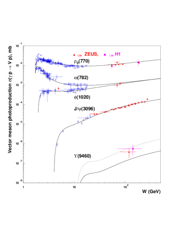
The results are presented in Fig. 2, which shows also the prediction of the model for $\Upsilon(9460)$ photoproduction.

Figure 2.  : Elastic cross-sections for vector meson photoproduction. The solid curve for $\Upsilon(9460)$ production corresponds to $N_{\Upsilon}=N_{\varphi}$, the dotted line to $N_{\Upsilon}=N_{J/\psi}$.

2.2 Photoproduction of vector mesons by virtual photons
($Q^{2}>0$).

In (17) and (19) the $Q^{2}$- dependence ($\tilde{Q}^{2}=Q^{2}+M_{V}^{2}$) is completely fixed up to an a priori arbitrary dimensionless function $f(Q^{2})$ such that $f(0)=1$. Thus, we may introduce a new factor that differentiates virtual from real photoproduction:

$$f(Q^{2})=\Big{(}\frac{M_{V}^{2}}{\tilde{Q}^{2}}\Big{)}^{n}$$ (21)

Accordingly, in the case $Q^{2}\neq 0$ we use the following parametrizations for Pomeron couplings (compare with Eq. 17):

$$\hat{g}_{i}(t;\tilde{Q}^{2},M_{V}^{2})=f(Q^{2})g_{i}(t;\tilde{Q}^{2},M_{V}^{2}),\;i=0,1,$$ (22)

where, for the sake of completeness, we will examine three different choices for the asymptotic $Q^{2}$ behaviour of the Pomeron residue

Choice I

$$n=1,\qquad\sigma_{T}({Q^{2}\rightarrow\infty})\sim\frac{1}{Q^{8}}\;.$$ (23)

Choice II

$$n=0.5,\qquad\sigma_{T}({Q^{2}\rightarrow\infty})\sim\frac{1}{Q^{6}}\;.$$ (24)

Choice III

$$n=0.25,\qquad\sigma_{T}({Q^{2}\rightarrow\infty})\sim\frac{1}{Q^{5}}\;.$$ (25)

For the reggeon couplings we have

$$f_{IR}(Q^{2})=\Big{(}\frac{c_{1}M_{V}^{2}}{c_{1}M_{V}^{2}+Q^{2}}\Big{)}^{n_{2}}\;,$$ (26)

where $c_{1}$ is an adjustable parameter and $n_{2}=0.25,\;-0.25,\;-0.5$ for choice I, II, III.

Accordingly, in the case $Q^{2}\neq 0$ we use the following parametrizations for Reggeons couplings (compare with Eq. 19):

$$\hat{g}_{IR}(t;\tilde{Q}^{2},M_{V}^{2})=f_{IR}(Q^{2})g_{IR}(t;\tilde{Q}^{2},M_{V}^{2})\;.$$ (27)

The lack of data on the ratio $\sigma_{L}/\sigma_{T}$, especially in the high $Q^{2}$ domain, does not allow us to draw definite conclusions about its asymptotic behaviour. There may be several realizations of the model with different asymptotic behaviour of $\sigma_{L}/\sigma_{T}$ [2]. As a demonstration of such a possibility we use the following (most economical) parametrization for $R$ (which cannot be deduced from the Regge theory)

Choice I, II, III

$$R(Q^{2},M_{V}^{2})=\Big{(}\frac{cM_{V}^{2}+Q^{2}}{cM_{V}^{2}}\Big{)}^{n_{1}}-1$$ (28)

where $c$ and $n_{1}$ are adjustable parameters for choice I, II, III.

We have, thus, 3 additional adjustable parameters as compared with real photoproduction. In order to obtain the values of the parameters for the case $Q^{2}\neq 0$, we fit just the data on $\rho_{0}$ meson photoproduction in the region $0\leq Q^{2}\leq 35\;GeV^{2}$; the parameters for photoproduction by real photons are fixed.

The parameters thus obtained may be found in [15].

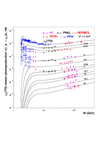
The results of the fit are depicted in Fig. 3. In this figure as well as in all following ones the solid lines, dashed lines and dotted lines correspond to the choice I, II, III correspondingly.

Figure 3.  : Elastic cross section of exclusive $\rho_{0}$ virtual photoproduction as a function of $W$ for different values of $Q^{2}$.

We can now check the predictions of the model. The $\chi^{2}/\#point=0.89$ for $J/\psi$ meson exclusive production follows without any fitting. Both $W$ and $Q^{2}$ dependences are reproduced very well. Notice that, so far, the three choices I, II, III all give equally acceptable reproduction of the data (see Figs. 5, 5 ).

Figure 4.  : Elastic cross section of exclusive $J/\psi$ virtual photoproduction as a function of $W$ for various $Q^{2}$.

Figure 5.  : Elastic cross section of exclusive $J/\psi$ virtual photoproduction as a function of $Q^{2}$ for $W=90\;GeV$.

We now plot the various ratios $\sigma_{L}/\sigma_{T}$ (these data were not fitted) corresponding to Eqs (23),(24),(25) (shown with the solid (choice I), dashed (choice II) and dotted (choice III) lines) in Fig. 8, 8, 8. The result shows, indeed, a rapid increase of $\sigma_{L}/\sigma_{T}$ with increasing $Q^{2}$, however one can see that our intermediate choice II is preferable to either I or III on this basis.

Let us examine the obtained dependences. We find that the data prefer

$$R(Q^{2}\rightarrow\infty)\sim\Big{(}\frac{Q^{2}}{M_{V}^{2}}\Big{)}^{n_{1}}\;,$$ (29)

where $n_{1}\simeq 2,\;1,\;0.3$ in choice I, II and III. Our, probably oversimplified, estimates and the data show $0.3<n_{1}<1$, see Fig. 8, thus $\sigma\sim 1/Q^{N}$ where $N\in(4,4.4)$ as $N=6-2n_{1}$ for the choice II and $N=5-2n_{1}$ for the choice III. However it is evident that new more precise data on $R$ are needed.

Figure 6.  : Ratio of $\sigma_{L}/\sigma_{T}$ for exclusive $\rho_{0}$ large $Q^{2}$ photoproduction.

Figure 7.  : Ratio of $\sigma_{L}/\sigma_{T}$ for exclusive $\varphi$ large $Q^{2}$ photoproduction.

Figure 8.  : Ratio of $\sigma_{L}/\sigma_{T}$ for exclusive $J/\psi$ large $Q^{2}$ photoproduction.

3 Conclusion

We have shown that the Soft Dipole Pomeron model recently developed [2], [15] for vector meson photoproduction allows us to describe well the new ZEUS data [1] on the differential and integrated cross-sections for $\gamma p\to J/\psi p$. Again, all available data on photoproduction of other vector mesons at $Q^{2}=0$ as well as $Q^{2}\neq 0$ are well reproduced.

The nonlinear Pomeron trajectory $\alpha_{P}(t)=1+\gamma\ (\sqrt{4m_{\pi}^{2}}-\sqrt{4m_{\pi}^{2}-t})$ turns out to be more suitable for the nonlinearity of the diffractive cone shown by the new ZEUS data.

We would like to emphasize the following important points

1. The Pomeron used in the model is a double pole in the complex $j$-plane with intercept which is equal to one

2. The new ZEUS data [1] (in contrast to the old ones) quite definitely point towards the nonlinearity of the Pomeron slope and trajectory.

3. Phenomenologically we find that in the region of available $Q^{2}$ the ratio $\sigma_{L}/\sigma_{T}\sim({Q^{2}}/{M_{V}^{2}})^{n_{1}}\;,$ where $0.3<n_{1}<1\;$. The definite conclusion can be derived only with new precise data on the ratio $\sigma_{L}/\sigma_{T}$, especially for high $Q^{2}$.

Acknowledgement

We would like to thank Michele Arneodo, Alexei Kaidalov, Alexander Borissov, Jean-Rene Cudell and Alessia Bruni for various and fruitful discussions. One of us (E.M.) would like to thank the Department of Theoretical Physics of the University of Torino for its hospitality and financial support during his visit to Turin.

References

• [1] ZEUS Collaboration: S. Chekanov et al., (2002)Eur.Phys.J. C 24, pp.345.
• [2] E.Martynov, A.Prokudin, E.Predazzi, (2001) hep-ph/0112242, to be published in Eur.Phys.J. C.
• [3] For a recent update on the Regge theory, see:
V. Barone, E. Predazzi (2002) “High-Energy Particle Diffraction”, Springer-Verlag Berlin Heidelberg
• [4] J.J. Sakurai, (1960) Ann. Phys. NY 11, pp.1;
M. Gell-Mann and F. Zacharaisen, (1961)Phys. Rev. D 124, pp.953.
• [5] D.E. Groom et al. (2000)Eur.Phys.J. C 15, pp.1.
• [6] J. Nemchik, N. N. Nikolaev, E. Predazzi and B. G. Zakharov (1997)Z. Phys. C 75, pp.71.
• [7] P.Desgrolard, M.Giffon, A.Lengyel, E.S.Martynov, (1994)Nuovo Cimento 107, pp.637.
• [8] J.R.Cudell et al., COMPETE Collaboration, (2002)Phys. Rev. D 65, pp.074024.
• [9] E.S.Martynov, (1994) Unitarization of Pomeron and Regge Phenomenology of Deep Inelastic Scattering. Proceedings of Workshop ”Hadrons-94”.
Kiev; Preprint (1994) ITP-94-49E, Kiev;
L.Jenkovszky, E.Martynov and F.Paccanoni, (1995) “Regge behaviour of the nucleon structure function”, Padova preprint, DFPD 95/TH/21.
• [10] M. Froissart, (1961)Phys. Rev. D 123, pp.1053;
A. Martin, (1963)Phys. Rev. D 129, pp.993.
• [11] A. Donnachie, P. V. Landshoff, (1987)Phys. Lett. B 185, pp.403;
A. Donnachie, P. V. Landshoff, (1995)Phys. Lett. B 348, pp.213.
• [12] L.L. Jenkovszky, E.S.Martynov, F.Paccanoni, (1996) “Regge Pole Model for Vector Meson Photoproduction at HERA”, hep-ph/9608384.
• [13] R. Fiore, L. L. Jenkovszky, F. Paccanoni (1999)Eur.Phys.J. C 10, pp.461; R. Fiore, L. L. Jenkovszky, F. Paccanoni, A. Papa (2002)Phys. Rev. D 65, pp.077505.
• [14] E. Predazzi, (1966)Ann. of Phys. (NY) 36, pp.250.
• [15] E.Martynov, A.Prokudin, E.Predazzi, (2002) hep-ph/0207272, submitted to Phys. Rev. D.