Symmetry Breaking and False Vacuum Decay after Hybrid Inflation

Abstract

We discuss the onset of symmetry breaking from the false vacuum in generic scenarios in which the mass squared of the symmetry breaking (Higgs) field depends linearly with time, as it occurs, via the evolution of the inflaton, in models of hybrid inflation. We show that the Higgs fluctuations evolve from quantum to classical during the initial stages. This justifies the subsequent use of real-time lattice simulations to describe the fully non-perturbative and non-linear process of symmetry breaking. The early distribution of the Higgs field is that of a smooth classical gaussian random field, and consists of lumps whose shape and distribution is well understood analytically. The lumps grow with time and develop into “bubbles” which eventually collide among themselves, thus populating the high momentum modes, in their way towards thermalization at the true vacuum. With the help of some approximations we are able to provide a quasi-analytic understanding of this process.

I Introduction

The problem of symmetry breaking in quantum field theory (QFT) has been with us for several decades. In the context of cosmology, it has usually been associated with thermal phase transitions KL , and the production of topological defects KZ . Understanding the way in which the order parameter associated with the breaking of the symmetry evolves from a symmetric state (the false vacuum) to a broken state (the true vacuum) is non-trivial CHKMPA ; BdV ; BHP ; AB ; Smit . Only recently has this problem been addressed in the context of symmetry breaking at zero temperature, at the end of a period of hybrid inflation hybrid ; GBL , in the so-called process of tachyonic preheating, i.e. spinodal instability, in the context of preheating after inflation KLS . There, classical evolution equations have been solved with real-time lattice simulations, developed for studying the problem of preheating TK ; PR ; FK , which include all the non-perturbative and non-linear character of the phase transition. It was found that symmetry breaking occurs typically in just one oscillation around the true vacuum GBKLT , most of the false vacuum energy going into gradient modes, rather than kinetic energy.

However, the problem of the transition from a false quantum vacuum state at zero temperature (as occurs at the end of a period of inflation) to the true quantum vacuum state full of radiation at a certain temperature has not been fully addressed yet. Most of the previous approaches refer to the decay from a false vacuum state at finite temperature, relying on the Hartree or large N approximation CHKMPA ; BdV ; AB ; Smit . Only recently, the zero temperature problem was addressed within the classical approximation but mainly for the case of an instantaneous quench GBKLT , which can lead to cosmologically interesting particle production GBRM . Tachyonic preheating was recently studied beyond the quench approximation in Ref. CPR .

We will argue that symmetry breaking proceeds through a state in which the relevant degrees of freedom are semi-classical infrared modes, which can be described in a non-perturbative and non-linear way with a classical effective field theory, whose classical equations of motion can be solved numerically in the lattice and thus allow us to study the fully non-perturbative out of equilibrium process of symmetry breaking.

The quantum to classical transitions of field Fourier modes have been addressed before in the context of inflation GuthPi ; PS ; KPS ; LPS , where it is mandatory to understand the transition from quantum fluctuations of the inflaton field during inflation to the classical metric fluctuations on super-horizon scales, since they are believed to be responsible for the observed temperature anisotropies in the cosmic microwave background, as well as the scalar density perturbations giving rise to galaxies and large scale structure formation. The use of the classical approximation to study the process of preheating after inflation has been proposed in TK , and, in a context similar to ours, it has been recently used in GBKLT ; CPR ; Smit .

In this paper we will use such a well developed formalism to study the first instances of a generic symmetry breaking process, i.e. the conversion of quantum modes of the symmetry breaking field (the QFT order parameter, generically called the Higgs field) into a classical gaussian random field whose subsequent non-linear evolution equations can be solved with lattice simulations. We give here a self-contained presentation of the conditions under which classical behaviour holds, and apply it to the analysis of the false vacuum decay after inflation, with specific initial conditions.

Our final aim is to study the process of electroweak symmetry breaking, and the possibility of realizing baryogenesis at the electroweak scale, via the non-equilibrium process of preheating after inflation GBKS ; KT ; RSC . Therefore, this paper is intended as the first one in a series, in which we will progressively incorporate more complexity, i.e. gauge fields, Chern-Simons, CP-violation, etc., into the picture. Of course, our results are readily generalisable to any other phase transition that may have occurred in the early universe at the end of a period of hybrid inflation, e.g. at GUT scales.

The paper is organised as follows. In Section II we describe the initial conditions for spontaneous symmetry breaking coming from a hybrid model of inflation. The inflaton acts here like a background field whose coupling gives a time-dependent mass to the Higgs. In Section III we study the quantum evolution of the Higgs field in the linear approximation from the bifurcation point. The Fourier modes decouple in this approximation and can be studied as a quantum mechanical ensemble of harmonic oscillators, both in the Heisenberg and the Schrödinger picture. We then study, with the use of the Wigner function, the quantum to classical transition of the Higgs modes. We show that each quantum mode can be described exactly like a classical gaussian random field, and give a prescription for computing the Weyl-ordered quantum expectation values of operators in terms of classical averages over a gaussian random field with the Wigner function as probability distribution. We then define and characterise when a mode can be called “quasi-classical”.

In Section IV we give the exact solutions to the field evolution equations of the Higgs in the linear approximation in terms of Airy functions, and show that soon after the bifurcation the infrared modes become quasi-classical according to the definition of the previous section. This analysis follows closely, although in greater detail, what has been studied previously in the literature ABC ; JGB ; CPR . In Section V we analyse the inclusion of the non-linear terms in the quantum evolution within perturbation theory. We give a prescription for treating the ultraviolet divergences and to renormalise the parameters of the theory. This leads to a regular probability distribution to be used for a classical field description, which matches the renormalised quantum expectation values of the Weyl ordered products. The matching is done at a time in which the infrared modes have grown sufficiently to be well described as classical modes. This occurs well before non-linearities are important, and therefore our gaussian approximation is valid, in a similar spirit as that of Ref. Smit . The quantum ultraviolet modes, on the contrary, can be thought as integrated out, and used to renormalise the parameters of the classical theory. We might then interpret our classical field distribution as an effective theory for the long wave-length modes. We also estimate the time at which symmetry breaking sets in.

In Section VI we describe the methodology to be used to take care of the full non-linear evolution of the system. The initial space-time structure of the classical Higgs field is analysed in VI.A. Being a gaussian random field, it can be described in a similar way to the matter density field whose fluctuations give rise to galaxies and large scale structure via gravitational collapse BBKS . The Higgs field is found to possess, at symmetry breaking, an inhomogeneous spatial distribution made of lumps, whose shape and initial evolution can be well understood analytically. The space-time inhomogeneous character of symmetry breaking in the Higgs-inflaton system has also been reported in Ref. CPR for a one component Higgs model. For the complete non-linear dynamics of the full Higgs-inflaton system we make use of lattice real-time evolution methods. The details of our procedure, its connection and difference with lattice methods used by other authors, and a detailed check of the validity of the approximations used, are described in Section VI.B.

Finally, in Section VII we present the results of this stage of the evolution of the system. The lumps mentioned in the previous sections grow and, once its center reaches the Higgs vacuum expectation value, invaginate and create an approximately spherically symmetric “bubble” which expands at a very high speed. Meanwhile, the center of the lump-bubble continues to oscillate with decreasing amplitude, leading to secondary bubbles. All these phenomena can be well understood with the help of some approximations which reduce the full non-linear equations to a one or two dimensional partial differential equation of a single scalar field. This simplified picture matches qualitatively and (to a high degree) quantitatively the results of the lattice simulations. Eventually, bubbles centred at different points collide and transfer most of their potential and kinetic energy to gradient energy, thus populating the higher momentum modes. This process leads to complete symmetry breaking and (classical) thermalization. The whole history of the system is illustrated by following the evolution of 2D sections of a particular configuration. We also show histograms for the field values of both Higgs and inflaton, which start in the false vacuum and are seen to end up peaked around the true vacuum. In Section VIII we draw our conclusions and describe the future directions in which this work can be extended, first by including the production of SU(2) gauge fields and afterwards by studying the rate of sphaleron transitions that may give rise to a non-negligible amount of baryons.

We have added three appendices. In Appendix A we describe the formalism of squeezed states following PS ; KPS , which can be applied to the initial stages of the Higgs evolution in the linear regime, and gives rise to the semi-classical nature of the long wavelength modes. In Appendix B we compute the Wigner function for the evolved gaussian initial vacuum state PS ; KPS ; LPS , and show explicitly the squeezing of the infrared modes. We give a definite condition for characterising the moment in which a mode can be treated as quasi-classical. In Appendix C we give the details of the perturbative calculations of the non-linear evolution of our system, both at a classical and quantum-mechanical level.

II The Higgs field at the end of hybrid inflation

The precise model of hybrid inflation will not be important for our purposes here. However, for concreteness we will implement it in the context of a super-symmetric extension of the standard model in which the radiative corrections are responsible for the running of the inflaton field during the few ($\sim 5-10$) e-folds necessary to cool the universe so that the electroweak symmetry breaking (EWSB) occurs at zero temperature. The fluctuations responsible for CMB temperature anisotropies and large scale structure come from a previous stage of inflation, completely independent of this. Moreover, since EWSB occurs at low energies, we can, and will in what follows, safely ignore the rate of expansion, $H\sim 10^{-5}$ eV, during symmetry breaking and treat the fields as if they were in Minkowski space. In particular, one can consider the super-symmetric hybrid model of Dvali, Shafi and Schaefer DSS , where the super-potential fixes a relation between the couplings, $g^{2}=2\lambda$. As we will see, this choice simplifies some stages of the dynamics of symmetry breaking after inflation BGK , but is not crucial. A study of the process of tachyonic preheating after a variety of more general super-symmetric models of inflation will be given in Ref. GBKL .

The hybrid model we are considering is a simple generalisation of the Standard Model symmetry breaking sector, which consists of the Higgs field, $\Phi={1\over 2}(\phi_{0}\,1\!{\rm l}+i\phi^{a}\tau_{a})$, with $\tau_{a}$ the Pauli matrices, and an inflaton $\chi$, a singlet under SU(2). The inflaton couples only to the Higgs, with coupling constant $g$. The scalar potential has the usual Higgs term plus a coupling to a massive inflaton,

$${\cal L}=(D_{\mu}\Phi)^{\dagger}\,D^{\mu}\Phi+{1\over 2}(\partial_{\mu}\chi)^{2}-\lambda\Big{(}\Phi^{\dagger}\Phi-{v^{2}\over 2}\Big{)}^{2}-g^{2}\chi^{2}\Phi^{\dagger}\Phi-{1\over 2}\mu^{2}\chi^{2}\,,$$ (1)

where $\,v=246$ GeV is the expectation value of the Higgs in the true vacuum, $\mu$ is the mass of the inflaton in the false vacuum and $m\equiv\sqrt{\lambda}\,v$. We are assuming implicitly that whenever there is a contraction $O^{\dagger}O$, we should take the trace over the SU(2) matrices, i.e. $\Phi^{\dagger}\Phi\equiv{\rm Tr}\,\Phi^{\dagger}\Phi={1\over 2}(\phi_{0}^{2}+\phi^{a}\phi_{a})\equiv|\phi|^{2}/2$. The Higgs mass in the true vacuum is determined by its self-coupling: $m_{\rm H}\equiv\sqrt{2\lambda}\,v$, while the mass of the inflaton in the true vacuum is given by $m_{\rm I}\equiv gv\gg\mu$.

In this paper we will simplify the analysis of the dynamics by omitting the $SU(2)$ gauge field and working with a generic Higgs field with $N_{c}$ real components. We anticipate that the most important conclusions of this paper are not affected by the introduction of the gauge field, and leave for a forthcoming publication the symmetry breaking dynamics in the presence of gauge fields. For ease of notation we will drop the internal indices of the Higgs field whenever all components behave in the same way. The numerical simulations that will be presented correspond to a $N_{c}=4$ component Higgs field.

During hybrid inflation hybrid the Higgs field has a large and positive effective mass squared due to its coupling to the inflaton field, which slow-rolls down its potential valley. The potential for the coupled fields is the following

$$V(\phi,\chi)={\lambda\over 4}\Big{(}|\phi|^{2}-v^{2}\Big{)}^{2}+{g^{2}\over 2}|\phi|^{2}\chi^{2}+{1\over 2}\,\mu^{2}\chi^{2}\,.$$ (2)

where the parameters in the potential depend on the number of Higgs components $N_{c}$ as: $\lambda=\lambda_{0}/N_{c}$, $g^{2}=g_{0}^{2}/N_{c}$ and $v^{2}=N_{c}\,v_{0}^{2}$, with this $m^{2}=\lambda v^{2}=\lambda_{0}v_{0}^{2}$ is independent of the number of components.

It is the effective false vacuum energy $V_{0}=\lambda v^{4}/4\equiv m^{2}v^{2}/4$ which drives the period of hybrid inflation. Inflation ends when the inflaton homogeneous mode, $\chi\equiv\langle\chi\rangle$, slow-rolls below the bifurcation point $\chi=\chi_{c}\equiv m/g$, at which the Higgs is massless,

$$m^{2}_{\phi}=m^{2}\,\Big{(}{\chi^{2}\over\chi_{c}^{2}}-1\Big{)}\,.$$ (3)

Below the critical point, the Higgs has a negative mass squared and long wave modes will grow exponentially, driving the process of symmetry breaking GBKLT . The process by which the mass squared of the Higgs goes from large and positive to large and negative is not instantaneous, but depends strongly on the velocity of the inflaton at the bifurcation point,

$$V\equiv{1\over m}\left|{\dot{\chi}\over\chi_{c}}\right|_{t_{c}}\,.$$ (4)

Typically the speed of the inflaton is such that the process takes place in less than one Hubble time, a condition known as the “waterfall” condition hybrid ; GBL , which ensures the absence of a second period of inflation after the bifurcation point GBLW . The actual value of $V$ depends very much on the model and the scale of inflation, and we will treat it here as an arbitrary model parameter. In this case, the effective mass of the Higgs across the bifurcation point can be written as a time-dependent mass

$$m^{2}_{\phi}(t)=-2V\,m^{3}(t-t_{c})+{\cal O}(V^{2}(t-t_{c})^{2})\,.$$ (5)

Note that a similar situation arises in the case of simple extensions of the standard model Higgs, in which radiative corrections (dominated by the large top quark Yukawa coupling) induce the running of the Higgs mass square from positive to negative thus providing a mechanism for Electroweak symmetry breaking. The role of the running scale is played here by the inflaton homogeneous mode. Alternatively, one can envisage a secondary period of hybrid thermal inflation LS ; review just above the electroweak scale, which lasted only a few $e$-folds and super-cooled the false vacuum, leaving only the fast rolling inflaton coupled to the Higgs. This short second period of inflation would not affect the CMB anisotropies, but would provide a natural initial condition for the growth of quantum fluctuation of the Higgs field, as they evolve across the bifurcation point, toward symmetry breaking.

Let us consider the effective action for the Higgs field $\Phi({\bf x},t)$ ignoring the self-coupling $\lambda$-term (we omit the internal indices of the Higgs field),

$${\cal S}=\int d^{3}{\bf x}\,dt\,{1\over 2}\left[(\dot{\phi})^{2}-(\nabla\phi)^{2}-m^{2}_{\phi}(t)\,\phi^{2}\right]\,,$$ (6)

where we have included the time-dependent mass (5), to linear order, which is the only effect that the presence of the homogeneous mode $\chi(t)$ of the inflaton field induces in the evolution of Higgs quantum modes.

We now define a new scale $M\equiv(2V)^{1/3}\,m$, and thus redefine our coordinates as

$$\tau = M\,(t-t_{c})\hskip 28.45274pt\longrightarrow\hskip 28.45274pt\dot{\phi}=M\,\phi^{\prime}\,,$$ (7)

$${\bf X} = M\,{\bf x}\hskip 56.9055pt\longrightarrow\hskip 28.45274pt{\bf K}={{\bf k}\over M}\,.$$ (8)

where primes denote derivatives w.r.t. $\tau$, and ${\bf k}$ is the wavenumber associated with the Higgs Fourier modes,

$$\Phi({\bf k},\tau)=\int{d^{3}{\bf x}\over(2\pi)^{3/2}}\,\Phi({\bf x},\tau)\,\exp(-i\,{\bf x}\cdot{\bf k})\,.$$

From now on, we will use ${\bf x}$ and ${\bf k}$ as the normalised position and momentum coordinates, i.e. we will work in units of $M=1$. We will also denote the normalised Higgs quantum fluctuations by $y=\phi/M$, for which the effective action is

$${\cal S}=\int d^{3}{\bf x}\,d\tau\,{1\over 2}\left[(y^{\prime})^{2}-(\nabla y)^{2}+\tau\,y^{2}\right]\,.$$ (9)

We can define the conjugate momentum as ${\displaystyle p={\partial{\cal L}\over\partial y^{\prime}}=y^{\prime}}\,,$ and thus the corresponding Hamiltonian becomes

$${\cal H}=\int d^{3}{\bf x}\,{1\over 2}\left[p^{2}+(\nabla y)^{2}-\tau\,y^{2}\right]\,.$$ (10)

In momentum space, the Hamiltonian becomes

$${\cal H}=\int d^{3}{\bf k}\,{1\over 2}\left[p({\bf k},\tau)\,p^{\dagger}({\bf k},\tau)+(k^{2}-\tau)\,y({\bf k},\tau)\,y^{\dagger}({\bf k},\tau)\right]\,.$$ (11)

The Euler-Lagrange equations for this field can be written in terms of the momentum eigenmodes as a series of uncoupled oscillator equations:

$$y^{\prime\prime}({\bf k},\tau)+(k^{2}-\tau)\,y({\bf k},\tau)=0\,.$$ (12)

III Quantum evolution in the gaussian approximation

In this section we will start the description of the quantum evolution of the system assuming that we can neglect the non-linear terms which are proportional to $\lambda$. Our goal is to determine the precise conditions under which the system evolves into a classical one. Our presentation will be general and applicable to any time dependent harmonic oscillator system with time-dependent spring constant $\omega^{2}(k,\tau)$, only in the next section we will apply this formalism to our particular problem ($\omega^{2}(k,\tau)=k^{2}-\tau$). Our results overlap and coincide with Refs. GuthPi ; PS ; KPS .

III.1 The Heisenberg picture

In the Heisenberg picture the quantum system is described by means of the position $y({\bf k},\tau)$ and momentum operators $p({\bf k},\tau)$ corresponding to each oscillator. The canonical equal-time commutation relations for the fields ($\hbar=1$ here and throughout) in position and momentum space are

$$\Big{[}y({\bf x},\tau),\ p({\bf x}^{\prime},\tau)\Big{]}=i\,\delta^{3}({\bf x}-{\bf x}^{\prime})\,,\hskip 42.67912pt\Big{[}y({\bf k},\tau),\ p({\bf k}^{\prime},\tau)\Big{]}=i\,\delta^{3}({\bf k}+{\bf k}^{\prime})$$ (13)

Furthermore, hermiticity of the operators in position space imply the relations $y^{\dagger}({\bf k},\tau)=y(-{\bf k},\tau)$ and $p^{\dagger}({\bf k},\tau)=p(-{\bf k},\tau)$

We will assume that at $\tau=\tau_{0}=0$, i.e. at the bifurcation point $t=t_{c}$, the state of the system is given by the ground state of the Hamiltonian with oscillator frequency $\omega(k,0)=k$. It is then useful to express the position and momentum operators in terms of creation-annihilation operators at that time:

$$\begin{array}[]{l}{\displaystyle y({\bf k},\tau_{0})={1\over\sqrt{2k}}\,\Big{(}a({\bf k},\tau_{0})+a^{\dagger}(-{\bf k},\tau_{0})\Big{)}}\,,\\[8.53581pt] {\displaystyle p({\bf k},\tau_{0})=-i\,\sqrt{k\over 2}\,\Big{(}a({\bf k},\tau_{0})-a^{\dagger}(-{\bf k},\tau_{0})\Big{)}}\,.\end{array}$$ (14)

The quantum operators satisfy the classical equations of motion, which we will write down as a system of coupled first-order equations

$${d\over d\tau}v({\bf k},\tau)\equiv{d\over d\tau}\pmatrix{p({\bf k},\tau)\vspace{2mm}\cr y({\bf k},\tau)}=\pmatrix{0&-\omega^{2}(k,\tau)\vspace{2mm}\cr 1&0}\pmatrix{p({\bf k},\tau)\vspace{2mm}\cr y({\bf k},\tau)}$$ (15)

whose solution can be expressed as:

$$v({\bf k},\tau)={\mathbf{M}}(k,\,\tau)\,v({\bf k},\tau_{0})\equiv\pmatrix{\sqrt{2\over k}\,g_{k1}(\tau)&\sqrt{2k}\,g_{k2}(\tau)\vspace{2mm}\cr-\sqrt{2\over k}\,f_{k2}(\tau)&\sqrt{2k}\,f_{k1}(\tau)}\,v({\bf k},\tau_{0})\,,$$ (16)

where $f_{k1}\equiv{\rm Re}\,f_{k}$ and $f_{k2}\equiv{\rm Im}\,f_{k}$, with $f_{k}(\tau)$ a complex solution of the equation of motion, with initial conditions,

$$f_{k}^{\prime\prime}+\Big{(}\omega(k,\tau)\Big{)}\,f_{k}=0\,,\hskip 28.45274ptf_{k}(\tau_{0})={1\over\sqrt{2k}}\,,$$ (17)

and

$$g_{k}\equiv g_{k1}+ig_{k2}=i\,f_{k}^{\prime}\,,\hskip 28.45274ptg_{k}(\tau_{0})=\sqrt{k\over 2}\,.$$ (18)

Note that since the motion is Hamiltonian (i.e. canonical), the determinant of ${\mathbf{M}}(k,\,\tau)$ is $\det\,{\mathbf{M}}(k,\,\tau)=1\,,\forall\tau$, a condition that is equivalent to the Wronskian of Eq. (17) being one at all times,

$$i\,(f_{k}^{\prime}\,f_{k}^{*}-{f_{k}^{\prime}}^{*}f_{k})=g_{k}\,f_{k}^{*}+g_{k}^{*}\,f_{k}=2\,{\rm Re}\,(g_{k}\,f_{k}^{*})=1\,.$$ (19)

The previous formulae allow us to compute the expectation value of products of fields at any time $\tau$ in terms of the expectation values of fields at time $\tau_{0}$. Substituting (14) into the expression for the fields at time $\tau$ we obtain

$$\begin{array}[]{l}y({\bf k},\tau)=f_{k}(\tau)\,a({\bf k},\tau_{0})+f_{k}^{*}(\tau)\,a^{\dagger}(-{\bf k},\tau_{0})\,,\\[8.53581pt] p({\bf k},\tau)=-i\,\Big{(}g_{k}(\tau)\,a({\bf k},\tau_{0})-g_{k}^{*}(\tau)\,a^{\dagger}(-{\bf k},\tau_{0})\Big{)}\,.\end{array}$$ (20)

The quantum information of the system is encoded in the expectation values of products of fields. For a gaussian field the only quantities needed to describe the system are the two-point expectation values,

$$\langle 0,\tau_{0}|v_{a}({\bf k},\tau)\,v_{b}({\bf k}^{\prime},\tau^{\prime})|0,\tau_{0}\rangle=\Sigma_{ab}(k,\tau,\tau^{\prime})\,\delta^{3}({\bf k}+{\bf k}^{\prime})\,,$$ (21)

where $|0,\tau_{0}\rangle$ is the initial vacuum state satisfying $a({\bf k},\tau_{0})|0,\tau_{0}\rangle=0\,,\forall{\bf k}$. The value of this matrix at any pair of times can be expressed in terms of the matrix ${\mathbf{M}}$ and the corresponding expectation values at time $\tau_{0}$ as follows:

$$\Sigma(k,\tau,\tau^{\prime})={\mathbf{M}}(k,\,\tau)\,\Sigma(k,\tau_{0},\tau_{0})\,{\mathbf{M}}^{T}(k,\,\tau^{\prime})\,.$$ (22)

The quantum initial condition on the state of the system at time $\tau_{0}$ amounts to:

$$\Sigma(k,\tau_{0},\tau_{0})=\pmatrix{{k\over 2}&-{i\over 2}\vspace{2mm}\cr{i\over 2}&{1\over 2k}}\,.$$ (23)

Note that this matrix is hermitian, but neither real nor symmetric, and its determinant vanishes. The imaginary part results from the equal time commutation relations and does not depend on the particular state of the system. The real symmetric part alone characterises completely the state.

Let us conclude this section by giving the expression of the equal time expectation values at any other time:

$$\Sigma(k,\tau,\tau)=\pmatrix{|g_{k}(\tau)|^{2}&F_{k}(\tau)-{i\over 2}\vspace{3mm}\cr F_{k}(\tau)+{i\over 2}&|f_{k}(\tau)|^{2}}=\pmatrix{|g_{k}(\tau)|^{2}&-i\,\Omega_{k}^{*}(\tau)|f_{k}(\tau)|^{2}\vspace{3mm}\cr i\,\Omega_{k}(\tau)|f_{k}(\tau)|^{2}&|f_{k}(\tau)|^{2}}$$ (24)

with

$$\Omega_{k}(\tau) = {g_{k}^{*}(\tau)\over f_{k}^{*}(\tau)}={1-2i\,F_{k}(\tau)\over 2|f_{k}(\tau)|^{2}}\,,$$ (25)

$$F_{k}(\tau) = {\rm Im}\,(f_{k}^{*}\,g_{k})\,.$$ (26)

As a consequence of the unit determinant of ${\mathbf{M}}(k,\,\tau)$ one concludes that the determinant of the symmetric (real) part of $\Sigma(k,\tau,\tau)$ is time-independent and equal to $1/4$. Note that using (25) we can rewrite the conjugate momentum as

$$p({\bf k},\tau)=\bar{p}({\bf k},\tau)+{F_{k}(\tau)\over|f_{k}(\tau)|^{2}}\,y({\bf k},\tau)$$ (27)

with

$$\bar{p}({\bf k},\tau)=-{i\over|f_{k}(\tau)|^{2}}\,\Big{(}f_{k}(\tau)\,a({\bf k},\tau_{0})-f_{k}^{*}(\tau)\,a^{\dagger}(-{\bf k},\tau_{0})\Big{)},$$

a relation that will prove useful in the next section.

III.2 The Schrödinger picture and the classical limit

Let us go now from the Heisenberg to the Schrödinger representation, and compute the initial state vacuum eigenfunction $\Psi_{0}(\tau=\tau_{0})$. We will follow here Refs. GuthPi ; PS ; KPS . In what follows we will denote operators in the Schrödinger representation by $\hat{y}_{\bf k}\equiv y({\bf k},\tau_{0})$ and $\hat{p}_{\bf k}\equiv p({\bf k},\tau_{0})$. The initial vacuum state $|0,\tau_{0}\rangle$ is defined through the condition

$$\forall{\bf k}\,,\hskip 28.45274pt\hat{a}({\bf k},\tau_{0})|0,\tau_{0}\rangle=\left[\sqrt{k\over 2}\,\hat{y}_{\bf k}+i\,{1\over\sqrt{2k}}\,\hat{p}_{\bf k}\right]|0,\tau_{0}\rangle=0\,,\hskip 28.45274pt$$

$$\left[y_{k}^{0}+{1\over k}\,{\partial\over\partial{y_{k}^{0}}^{*}}\right]\Psi_{0}\Big{(}y_{k}^{0},{y_{k}^{0}}^{*},\tau_{0}\Big{)}=0\hskip 14.22636pt\Rightarrow\hskip 14.22636pt\Psi_{0}\Big{(}y_{k}^{0},{y_{k}^{0}}^{*},\tau_{0}\Big{)}=N_{0}\,e^{-k\,|y_{k}^{0}|^{2}}\,,$$ (28)

where we have used the position representation, $\hat{y}_{\bf k}=y_{k}^{0}\,,\ \hat{p}_{\bf k}=-i\,{\partial\over\partial{y_{k}^{0}}^{*}}$, and $N_{0}$ gives the corresponding normalisation.

We will now study the time evolution of this initial wave function using the unitary evolution operator ${\cal U}={\cal U}(\tau,\tau_{0})$, satisfying ${\cal U}^{\prime}=-i\,{\cal H\,U}$. The state evolves in the Schrödinger picture as $|0,\tau\rangle={\cal U}|0,\tau_{0}\rangle$. We can make use of the result of the previous section to determine this state. By inverting (20) we find

$$\hat{a}({\bf k},\tau_{0})=g_{k}^{*}(\tau)\,\hat{y}({\bf k},\tau)+i\,f_{k}^{*}(\tau)\,\hat{p}({\bf k},\tau)\,,$$ (29)

which acting on the initial state becomes, $\forall{\bf k}\,,\forall\tau$,

$${\cal U}\left[\hat{y}({\bf k},\tau)+i\,{f_{k}^{*}(\tau)\over g_{k}^{*}(\tau)}\,\hat{p}({\bf k},\tau)\right]{\cal U}^{\dagger}{\cal U}|0,\tau_{0}\rangle=\left[\hat{y}_{\bf k}+i\,{f_{k}^{*}(\tau)\over g_{k}^{*}(\tau)}\,\hat{p}_{\bf k}\right]\!|0,\tau\rangle=0\,,$$

$$\Rightarrow\hskip 28.45274pt\Psi_{0}\Big{(}y_{\bf k}^{0},{y_{\bf k}^{0}}^{*},\tau\Big{)}\,=\,{e^{-i\alpha}\over\sqrt{\pi}\,|f_{k}(\tau)|}\,e^{-\Omega_{k}(\tau)\,|y_{k}^{0}|^{2}}\,,\hskip 85.35826pt$$ (30)

with $\Omega_{k}(\tau)$ given by Eq. (25). We see that the unitary evolution preserves the gaussian form of the wave functional. The wave function (30) is called a 2-mode squeezed state. The normalised probability distribution, for each mode $k$,

$$P_{0}\Big{(}y_{k}^{0},{y_{k}^{0}}^{*},\tau\Big{)}={1\over\pi\,|f_{k}(\tau)|^{2}}\,\exp\Big{(}-{|y_{k}^{0}|^{2}\over|f_{k}(\tau)|^{2}}\Big{)}\,,$$ (31)

is a gaussian distribution, with dispersion given by $|f_{k}|^{2}$. This agrees with the result obtained in the previous section in the Heisenberg picture. The phase $\alpha(k,\tau)$ cannot be determined by this method, but as we have seen it has no effect on the probability distribution nor on the Wigner function, see below. However, from the Schrödinger equation, $i\partial_{\tau}\Psi_{0}(\tau)={\cal H}\Psi_{0}(\tau)$, one can deduce that $\alpha^{\prime}(k,\tau)=(2|f_{k}(\tau)|^{2})^{-1}$.

We can also compute the occupation number, $n_{k}$,

$$n_{k}(\tau)=\langle 0,\tau|a^{\dagger}({\bf k},\tau_{0})a({\bf k},\tau_{0})|0,\tau\rangle={1\over 2k}|g_{k}|^{2}+{k\over 2}|f_{k}|^{2}-{1\over 2}\,,$$ (32)

a quantity that is always positive definite.

We now address the problem of approximating the quantum evolution just described by a classical evolution. For that purpose the vacuum expectation values of products of position and momentum operators should be recovered as ensemble averages of random fields. It is clear that for the non-interacting theory ($\lambda=0$) that we are considering, such a classical random field should be gaussian, with all the information encoded in the real expectation values of products of two fields. Only the symmetrical part of $\Sigma(k,\tau,\tau)$ is real, see (24), and thus a natural candidate to be approximated by the classical gaussian random field. Notice that this corresponds to matching Weyl-ordered (symmetrised in $\hat{y}_{\bf k}$, $\hat{p}_{\bf k}^{\dagger}$) quantum expectation values of operators through, in the Schrödinger picture,

$$\langle 0,\tau|G(\hat{y}_{\bf k},\hat{p}_{\bf k})|0,\tau\rangle_{W}\equiv\langle G(y_{\bf k},p_{\bf k})\rangle_{\rm gs}$$ (33)

where $\langle 0,\tau|G(\hat{y}_{\bf k},\hat{p}_{\bf k})|0,\tau\rangle_{W}$ denotes the quantum average of the Weyl-ordered operator in the state given by the wave function (30), and $\langle G(y_{\bf k},p_{\bf k})\rangle_{\rm gs}$ denotes the classical gaussian average. The latter is obtained as an average over a gaussian ensemble with $y_{\bf k}$ and ${\displaystyle\bar{p}_{\bf k}\Big{(}\equiv p_{\bf k}-{F_{k}(\tau)\over|f_{k}(\tau)|^{2}}\,y_{\bf k}\Big{)}}$ independent gaussian variables with probability distribution given by the Wigner function in phase space, see PS ; KPS , equation (27) and the Appendix B

$$W_{0k}(y,p)={1\over\pi^{2}}\,\exp\left(-{|y|^{2}\over|f_{k}|^{2}}-4|f_{k}|^{2}\Big{|}p-{F_{k}\over|f_{k}|^{2}}\,y\Big{|}^{2}\right)\ .$$ (34)

A very trivial illustration of this equality is given by the following symmetrised vacuum expectation value

$${1\over 2}\,\langle 0,\tau|\,\hat{y}_{\bf k}\,\hat{p}_{{\bf k}^{\prime}}+\hat{p}_{\bf k}\,\hat{y}_{{\bf k}^{\prime}}\,|0,\tau\rangle=F_{k}(\tau)\delta^{3}({\bf k}+{\bf k}^{\prime})$$ (35)

while

$$\langle\,y_{\bf k}\,p_{{\bf k}^{\prime}}\,\rangle_{\rm gs}=\langle\,y_{\bf k}\,(\,\bar{p}_{{\bf k}^{\prime}}+{F_{k}(\tau)\over|f_{k}|^{2}}\,y_{{\bf k}^{\prime}}\,)\,\rangle_{\rm gs}={F_{k}(\tau)\over|f_{k}|^{2}}\,\langle\,y_{\bf k}\,y_{{\bf k}^{\prime}}\,\rangle_{\rm gs}=F_{k}(\tau)\,\delta^{3}({\bf k}+{\bf k}^{\prime})\,.$$ (36)

Even though only the symmetrised expectation values are described by the gaussian ensemble average, for the gaussian ground state of (30) quantum expectation values with arbitrary ordering of operators can also be computed. To be specific, the expectation value of any operator $G(\hat{y},\hat{p})$, with any given ordering of $\hat{y}$ and $\hat{p}$, can be rewritten as a lineal combination of Weyl-ordered operators with coefficients proportional to the commutator which is a time independent c-number; schematically

$$\langle 0,\tau|G(\hat{y},\hat{p})|0,\tau\rangle=\langle G_{0}(y,p)\rangle_{\rm gs}\,+\sum_{n\geq 1}\,(i\hbar)^{n}\,\langle G_{n}(y,p)\rangle_{\rm gs}\,,$$ (37)

where we have introduced $\hbar$ as an expansion parameter to make explicit the connection with the semi-classical approximation. For instance, for the example in (35) we would obtain

$$\langle 0,\tau|\,\hat{y}_{\bf k}\,\hat{p}_{{\bf k}^{\prime}}\,|0,\tau\rangle=\Big{(}F_{k}(\tau)-{i\over 2}\Big{)}\,\delta^{3}({\bf k}+{\bf k}^{\prime})$$ (38)

In this spirit, a quasi-classical state can be defined as a state for which the leading term in equation (37) dominates, and quantum averages can be approximated by

$$\langle 0,\tau|\,G(\hat{y},\hat{p})\,|0,\tau\rangle\approx\langle\,G_{0}(y,p)\,\rangle_{\rm gs}.$$ (39)

This generically happens when $\langle 0,\tau|\,\hat{p}\,\hat{y}\,|0,\tau\rangle_{W}\gg|\langle 0,\tau|\,[\,\hat{p},\hat{y}\,]\,|0,\tau\rangle|$, i.e. when the so-called WKB phase, $F_{k}(\tau)$ in (26), verifies $|F_{k}(\tau)|\gg 1$. For such a quasi-classical state the ambiguity in the ordering of operators is quantitatively negligible and classicality in the sense of (39) holds. As an illustration let us compute the following expectation value (for ease of notation we have omitted the ${\bf k}$ dependence of the operators and the delta functions)

$${1\over 2}\,\langle 0,\tau|\,\hat{p}^{2}\,\hat{y}^{2}\,+\,\hat{y}^{2}\,\hat{p}^{2}\,|0,\tau\rangle=3F_{k}^{2}(\tau)-{1\over 4}.$$ (40)

In the classical approximation we would obtain

$$\langle\,p^{2}\,y^{2}\,\rangle_{\rm gs}=\langle\,p^{2}\,\rangle_{\rm gs}\,\langle\,y^{2}\,\rangle_{\rm gs}+\,2\langle\,p\,y\,\rangle_{\rm gs}^{2}=|f_{k}(\tau)|^{2}|g_{k}(\tau)|^{2}+2F_{k}^{2}(\tau)=3F_{k}^{2}(\tau)+{1\over 4}$$ (41)

which reproduces the Weyl ordered part of the quantum result and is a very good approximation as long as $|F_{k}(\tau)|\gg 1$.

This approach works as long as the theory is non-interacting and the gaussianity of the quantum state is preserved by the evolution. In the problem at hand, we can assume this to be the case in the first stages of evolution before non linearities have set in, but not when the self-coupling term starts to be relevant just before symmetry breaking. However, as long as $|F_{k}(\tau)|\gg 1$, the state can still be approximately described, through the non-linear stages, via a classical random field. We will describe below in detail how this classicality follows for our specific problem (see also the Appendices A and B for the precise formulation of the squeezed states and the Wigner function formalism, following Refs. PS ; KPS ; LPS ).

IV Exact solutions of the field evolution equations

Let us apply now the above formalism to the case of the quantum fluctuation modes of the Higgs at symmetry breaking. This case was studied previously in BM ; ABC ; JGB ; CPR . For $\omega^{2}(k,\tau)=k^{2}-\tau$ the linear equation (17) for the quantum modes of the Higgs field becomes

$$f_{k}^{\prime\prime}+(k^{2}-\tau)\,f_{k}=0\,,\hskip 28.45274pt{\rm with}\hskip 14.22636ptf_{k}(\tau_{0}=0)={1\over\sqrt{2k}}\,.$$ (42)

Its solution can be given in terms of Airy functions AS :

$$f_{k}(\tau) = C_{1}(k)\,{\rm Bi}(\tau-k^{2})+C_{2}(k)\,{\rm Ai}(\tau-k^{2})\,,$$ (43)

$$g_{k}(\tau) = i\,C_{1}(k)\,{\rm Bi}^{\prime}(\tau-k^{2})+i\,C_{2}(k)\,{\rm Ai}^{\prime}(\tau-k^{2})\,,$$ (44)

$$C_{1}(k) = -{\pi\over\sqrt{2k}}\,\Big{[}{\rm Ai}^{\prime}(-k^{2})+ik\,{\rm Ai}(-k^{2})\Big{]}\,,$$ (45)

$$C_{2}(k) = {\pi\over\sqrt{2k}}\,\Big{[}{\rm Bi}^{\prime}(-k^{2})+ik\,{\rm Bi}(-k^{2})\Big{]}\,,$$ (46)

which satisfy the Wronskian condition, $g_{k}\,f_{k}^{*}+g_{k}^{*}\,f_{k}=1$, where we have used the corresponding Wronskian for the Airy functions,

$$\pi\,[{\rm Ai}(z){\rm Bi}^{\prime}(z)-{\rm Bi}(z){\rm Ai}^{\prime}(z)]=1\,.$$ (47)

We can then compute the occupation number, $n_{k}$, (32) and the imaginary part of the WKB phase, $F_{k}$, see (26).

IV.1 Long wavelength quasi-classical modes

Still remains to be computed the time at which fluctuations become classical in the sense of Eq. (39). As we will see, the field fluctuation modes will become quasi-classical as their wavelength becomes larger than the only physical scale in the problem, the time-dependent Higgs mass, i.e. $\lambda=2\pi/k\gg 2\pi/\sqrt{\tau}$. In order to show this, let us take the limit $k^{2}\ll\tau$ for the long wavelength modes in the exact solutions (43) and (44),

$$f_{k}(\tau) = C_{1}(k)\,{\rm Bi}(\tau)+C_{2}(k)\,{\rm Ai}(\tau)\ \simeq\ C_{1}(k)\,w(\tau)\,,$$ (48)

$$g_{k}(\tau) = iC_{1}(k)\,{\rm Bi}^{\prime}(\tau)+iC_{2}(k)\,{\rm Ai}^{\prime}(\tau)\ \simeq\ i\,C_{1}(k)\,w^{\prime}(\tau)\,,$$ (49)

where the function $w(\tau)={\rm Bi}(\tau)+\sqrt{3}\,{\rm Ai}(\tau)$ is the one appearing in the Appendix A, and we have used the fact that $C_{2}(k)=\sqrt{3}\,C_{1}(k)$ in the limit $k\to 0$. Using the large $z\mathrel{\mathop{\hbox{\lower 2.15277pt\hbox{$\sim$}\kern-8.00003pt\lower-3.01385pt\hbox{$>$}}}}1$ approximation of the Airy functions, see Ref. AS ,

$${\rm Bi}(z)\sim{1\over\sqrt{\pi}}\,z^{-1/4}\,e^{+{2\over 3}z^{3/2}}\,, \hskip 28.45274pt{\rm Ai}(z)\sim{1\over 2\sqrt{\pi}}\,z^{-1/4}\,e^{-{2\over 3}z^{3/2}}\,,$$ (50)

$${\rm Bi}^{\prime}(z)\sim z^{1/2}\,{\rm Bi}(z)\,,\hskip 34.14322pt \hskip 5.69054pt{\rm Ai}^{\prime}(z)\sim-z^{1/2}\,{\rm Ai}(z)\,,$$ (51)

we conclude that the first terms in both $f_{k}$ and $g_{k}$ correspond to the growing modes, while the second terms are the decaying modes, and can be ignored soon after the bifurcation point.

We are now prepared to answer the question of classicality of the modes. The wave function phase shift is given by

$$F_{k}={\rm Im}\,(f_{k}^{*}\,g_{k})\simeq|C_{1}(k)|^{2}\,w^{\prime}(\tau)\,w(\tau)\simeq{w^{\prime}(\tau)\over w(\tau)}\,|f_{k}|^{2}\simeq|C_{1}(k)|^{2}\,{1\over\pi}\,e^{{4\over 3}\tau^{3/2}}\,,$$ (52)

which grows faster than exponentially at large time. On the other hand, the occupation number (32) is

$$2k\Big{(}n_{k}+{1\over 2}\Big{)}=|g_{k}|^{2}+k^{2}\,|f_{k}|^{2}\simeq\Big{(}{w^{\prime}(\tau)\over w(\tau)}\Big{)}^{2}\,|f_{k}|^{2}\simeq\sqrt{\tau}\,|C_{1}(k)|^{2}\,{1\over\pi}\,e^{{4\over 3}\tau^{3/2}}\,.$$ (53)

Therefore, we have

$$|F_{k}(\tau)|\simeq{2k\,n_{k}(\tau)\over(w^{\prime}/w)}\gg 1\hskip 14.22636pt\longrightarrow\hskip 14.22636ptE_{k}(\tau)\simeq k\,n_{k}(\tau)\gg|m(\tau)|\,,$$ (54)

that is, $|F_{k}|\gg 1$ whenever the energy of the mode $E_{k}$ is much greater than the Higgs mass, computed as the instantaneous curvature of the Higgs potential.

Notice in particular that under the condition $|F_{k}|\gg 1$, the momentum and field eigenmodes are related by

$$g_{k}(\tau)=\Omega^{*}_{k}(\tau)f_{k}(\tau)\ \longrightarrow\ i{F_{k}(\tau)\over|f_{k}(\tau)|^{2}}f_{k}(\tau)\,.$$

In terms of the gaussian random fields, the momentum distribution of the Wigner function becomes a delta function, ${\displaystyle\delta\Big{(}p-{F_{k}(\tau)\over|f_{k}|^{2}}y\Big{)}}$, see Appendix B.

Figure 1: We compare the phase $|F_{k}|$ with the occupation number for different times, in the whole range of interest in momenta $k$. Clearly, for large times $\tau\gg 1$, the two coincide, as discussed in the text. Note that, after $\tau\simeq 2$, all long wavelength modes are essentially classical, $|F_{k}|\gg 1$.

Figure 2: The time for which a given mode $k$ can be treated as classical $|F_{k}(\tau_{\rm cl})|\equiv 1$ is above the line in this figure. It is clear that long wavelength modes with $0<k\mathrel{\mathop{\hbox{\lower 2.15277pt\hbox{$\sim$}\kern-8.00003pt\lower-3.01385pt\hbox{$<$}}}}1$ become classical very early, at $\tau_{\rm cl}\simeq 2$, while there remains, at any given time, a high energy spectrum of quantum modes, for $k\gg 1$.

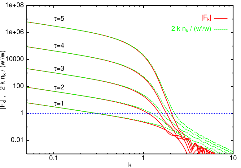
We show in Fig. 1 the exponential growth of the phase $F_{k}(\tau)$ as a function of momenta $k$, for different times. These plots were obtained using the exact Airy function solutions. Note that in the limit of large wavelengths $k^{2}\ll\tau$, it is indeed verified that $|F_{k}(\tau)|\simeq 2k\,n_{k}(\tau)(w/w^{\prime})\gg 1$, as stated above.

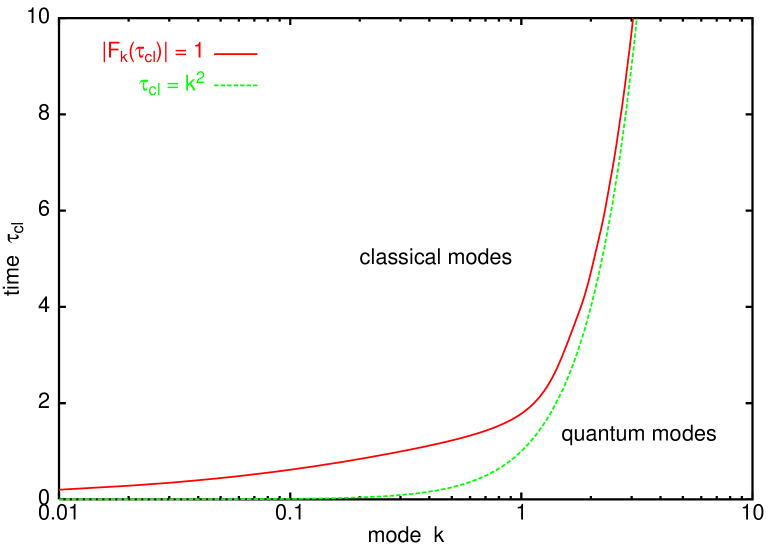
We can now compute the time for which a single mode $k$ becomes quasi-classical, in the sense (54). We have confirmed that after $\tau\simeq 2$ modes with $0\leq k<\sqrt{\tau}$ , which, as we will see later, is the range of interest, have become quasi-classical. We have drawn the line separating classical from quantum modes in Fig. 2, as a function of the mode $k$. The high energy part of the spectrum always remains in the quantum vacuum, as expected. For $\tau\geq 2$ the line separating classical and quantum modes is approximately described by $k=\sqrt{\tau}$.

V Non-linear quantum evolution and symmetry breaking

To address the issue of symmetry breaking after inflation it is essential to incorporate the non-linear effects proportional to $\lambda$. A full non-perturbative quantum treatment is beyond reach. However, we have seen in the previous section that the dynamics in the absence of non-linear terms gives rise to a fast growth of the amplitude of the low-lying momenta, leading to wave-functions which are squeezed (quasi-classical in our language). We argue that even when the interaction is switched on the dynamics of these modes dominates the evolution of the system (at least during the first stages), and that this dynamics is described by classical field theory. The argument does not apply to higher momentum modes which sit largely in the quantum mechanical ground state. However, in quantum field theory, high momentum modes, although small, do not give negligible contribution to observables. Actually, naively their contribution is divergent. Nevertheless, we argue that the main contribution of the small quantum mechanical high-momentum modes sits in the renormalization of the constants to be used in the classical theory.

It is possible to partially test this scheme in perturbation theory. Already at this stage the problem of infinities and renormalization arises BHP . In this section we will summarily analyse this issue, relegating the details of the calculations to the Appendix C. As we will see, for the program to be consistent one has to allow for a renormalization of the speed $V$ of the inflaton at the bifurcation.

In the standard setting, infinities in observables occur through the contribution of the infinite tower of momentum states. Introducing a cut-off in the problem makes the results finite, but cut-off dependent. It turns out, however, that in renormalizable theories, the only surviving effects of the cut-off at scales much smaller than itself are the modification of the constants of the theory. This allows the process of renormalization in which we recover uniqueness of the theory at the expense of taking this constants from experiment. We will now reexamine this problem for our time-dependent situation. Several research groups have investigated this problem in the past in different contexts, see CHKMPA ; BdV ; BHP ; ASm .

All the physical content of the theory is contained in the expectation values of products of the field operator at equal or different space-time points (we use the Heisenberg picture and expectation values should be understood as taken in the vacuum at $\tau=\tau_{0}$):

$$\langle y(\tau_{1},{\bf x}_{1})\ldots y(\tau_{n},{\bf x}_{n})\rangle\,.$$ (55)

By differentiating with respect to $\tau$ one can obtain expectation values of products of $y$ and $p$. If we were to compute these quantities in the gaussian (non-interacting) theory, we would obtain, via Wick’s theorem, a sum over all pairings of a product of factors associated to each pair

$$G^{(0)}(\tau,\tau^{\prime},{\bf x}-{\bf x}^{\prime})\equiv\langle y_{0}(\tau,{\bf x})y_{0}(\tau^{\prime},{\bf x}^{\prime})\rangle=\int\frac{d^{3}{\bf k}}{(2\pi)^{3}}e^{i{\bf k}({\bf x}-{\bf x}^{\prime})}\,f_{k}(\tau)f^{*}_{k}(\tau^{\prime})\,,$$ (56)

where $y_{0}$ denotes the gaussian field for $\lambda=0$. The gaussian two-point function is the Fourier transform of $\Sigma_{22}(k,\tau,\tau^{\prime})$ and is finite provided ${\bf x}\neq{\bf x}^{\prime}$ and/or $\tau\neq\tau^{\prime}$.

The correlation functions at different times (i.e. Wightman functions) can be computed in perturbation theory by the method described in the Appendix C. Wightman functions are complex and unlike Feynman Green-functions (time-ordered products) depend on the order of the operators. According with our criterion for the gaussian case, we will consider Weyl-ordered (symmetrised) products to make the matching with the classical theory. If we now consider the symmetrised two-point function

$$\langle y({\bf x},\tau)y({\bf x}^{\prime},\tau^{\prime})\rangle_{W}=\int\frac{d^{3}{\bf k}}{(2\pi)^{3}}e^{i{\bf k}({\bf x}-{\bf x}^{\prime})}\,\hat{G}(k,\tau,\tau^{\prime})$$ (57)

we can compute it to first order in $\lambda$. The result is

$$\hat{G}(k,\tau,\tau^{\prime})={\rm Re}\,[f_{k}(\tau)f_{k}^{*}(\tau^{\prime})] + \,2(N_{c}+2)\lambda\int_{0}^{\tau}ds\,A(s)\,{\rm Im}\,[f_{k}(\tau)f_{k}^{*}(s)]\,{\rm Re}\,[f_{k}(\tau^{\prime})f_{k}^{*}(s)]$$

$$+ \,2(N_{c}+2)\lambda\int_{0}^{\tau^{\prime}}ds\,A(s)\,{\rm Im}\,[f_{k}(\tau^{\prime})f_{k}^{*}(s)]\,{\rm Re}\,[f_{k}(\tau)f_{k}^{*}(s)]\,.$$

where $N_{c}$ denotes the number of components of the Higgs field. The quantity $A(s)$ gives the contribution of the tadpole sub-diagram, i.e. the two-point function at equal times and zero distance, and is given by

$$A(\tau)\equiv G^{(0)}(\tau,\tau,0)=\int{d^{3}{\bf k}\over(2\pi)^{3}}\,|f_{k}(\tau)|^{2}={1\over 2\pi^{2}}\,\int{dk\over k}\,P(k,\tau)\,,$$ (59)

where the power spectrum is defined as $P(k,\tau)=k^{3}|f_{k}(\tau)|^{2}$. This quantity is ultraviolet divergent. The structure of the divergence can be deduced by analysing the large $k$ behaviour of the integrand. Using our previous expressions (with $z=k^{2}-\tau$) and the asymptotic behaviour of Airy functions AS we get

$$|f_{k}(\tau)|^{2}\simeq\,{1\over 2k}\left[1+{\tau\over 2k^{2}}\Big{(}1-{\sin(2k\tau)\over 2k\tau}\Big{)}+{\cal O}(\tau^{2})\right]\,,$$ (60)

$$P(k,\tau)=k^{3}|f_{k}(\tau)|^{2}\sim{k^{2}\over 2}+{\tau\over 4}\Big{(}1-{\sin(2k\tau)\over 2k\tau}\Big{)}+{\cal O}\Big{(}{\tau^{2}\over k}\Big{)}\,.$$ (61)

Thus $A(\tau)$ has a time-independent quadratic divergence and a linear in time logarithmic divergence.

Before explaining how can one deal with the divergence, we comment that Eqs. (57-V) coincide precisely with the calculation of the expectation values of the product of classical random field to the same order in perturbation theory. Divergences are hence present in both the quantum and the classical theory. Details of this calculation are also shown in Appendix C.

We now address the problem of infinities that have occurred at this level. In the standard quantum theory the procedure is well-known. The calculation can be done using some regulator to cut off the contributions of high momenta, but this has to be accompanied by the addition of counter-terms in the interaction Hamiltonian. For the theory to be renormalizable these counter-terms should have the same expression as those appearing in the Hamiltonian (free or interacting) but with coefficients which are cut-off dependent and proportional to some power of $\lambda$. This addition should get rid of infinities. Note that in our case a counter-term of the form

$$-{N_{c}+2\over 2}\lambda\Big{(}\delta_{1}(\Lambda)+\tau\,\delta_{2}(\Lambda)\Big{)}\,y_{0}^{2}({\bf x},\tau)\,,$$ (62)

with $\delta_{1}$ and $\delta_{2}$ appropriately chosen cut-off dependent functions, is able to subtract the infinities encountered in $A(t)$. Regularising the integrals by introducing a cut-off in momenta $k<\Lambda$ we then get:

$$A_{\mbox{\tiny ren}}(\tau,\mu)=A_{\mbox{\tiny reg}}(\tau,\Lambda)-\delta_{1}(\Lambda,\mu)-\tau\,\delta_{2}(\Lambda,\mu)$$ (63)

To fix the arbitrariness introduced in the theory by the counter-term we must impose adequate renormalization conditions. As will be argued below, one convenient possibility is to choose the counter-term as

$$\delta_{1}(\Lambda,\mu)+\tau\,\delta_{2}(\Lambda,\mu)={1\over 2\pi^{2}}\int_{\mu}^{\Lambda}dk\,k^{2}\,\Big{(}|f_{k}(\tau=\mu^{2})|^{2}\,+(\tau-\mu^{2})\,2\,F(\tau=\mu^{2})\Big{)}\,.$$ (64)

where $\mu$ denotes the characteristic mass scale of the problem which for a given time $\tau$ is precisely $\sqrt{\tau}$. We will call this renormalization prescription, the fixed-time subtraction scheme. Another possibility is a minimal subtraction scheme (not to be confused with the MS scheme of dimensional regularization)

$$A_{\mbox{\tiny ren}}(\tau,\mu)=A_{\mbox{\tiny reg}}(\tau,\Lambda)-{1\over 8\pi^{2}}\,\left(\Lambda^{2}+\tau\,\log{\Lambda\over\mu}\right)\,.$$ (65)

which differs from the previous one by finite terms of the form $a+b\tau$. Actually, the renormalised quantity is obtained only after taking the limit $\Lambda\rightarrow\infty$ in the subtracted quantity, but in practice taking $\Lambda$ sufficiently large is a good approximation.

The fact that the structure of the counter-terms (or of the divergence) has the same form as the terms already present in the Hamiltonian, shows that our calculation is consistent at least to this order. The infinities are re-absorbed in the values of the constants of the theory. Here, in addition to the ordinary time-independent subtraction we have a counter-term linear in $\tau$, which can be interpreted as a renormalization of $\chi-\chi_{c}$, i.e. of the inflaton velocity $V$. A different choice of scheme is compensated by a finite renormalization of the parameters of our model.

Now we look back at the problem of approximating the result by a classical random field. Since the regularised result to this order is the same (for symmetric expectation values) a similar subtraction procedure is necessary. There is certainly no problem to do so in perturbation theory. However, in practice what we want to do is to be able to match the renormalised quantum result by modifying the initial spectrum of the classical field to be used as starting point for the classical evolution. Notice that when $\tau=\tau_{i}=\mu^{2}$ the value of $A_{\mbox{\tiny ren}}$ obtained with the fixed-time subtraction scheme, (64), is exactly reproduced by truncating the initial spectrum at $\mu=\sqrt{\tau_{i}}$. This is a very natural choice from the point of view of the classical approximation. As can be seen from Figs. 1, 2, for large enough $\tau$ the separation between quantum and classical modes sits indeed at $k\simeq\sqrt{\tau}$. At a given time modes with momenta below $\sqrt{\tau}$ have been amplified while those above $\sqrt{\tau}$ remain in the vacuum. The amplification proceeds until some time $\tau_{\rm sb}$, when $\langle\phi^{2}(\tau_{\rm sb})\rangle$ gets close to the vacuum expectation value $v^{2}$ and the field starts oscillating around the true vacuum. The dynamics of symmetry breaking is hence expected to be governed by the low momentum modes with $k^{2}<\tau_{\rm sb}$ whose evolution can be described in the classical approximation (as we will see below for a large range of parameters, $\tau_{\rm sb}$ varies only within the values $\tau_{\rm sb}=5\pm 2$). The classical theory can then be seen, in a way analogous to what happens at high temperature ASm ; Hight , as an effective theory where momenta above $k_{*}=\sqrt{\tau_{\rm sb}}$ have been integrated out. As far as modes above $k_{*}$ are not highly populated by rescattering and back-reaction this effective theory is expected to be valid and can be studied within the classical approximation.

In summary, our proposal is to fix our classical field by matching its correlation functions with the renormalised perturbative expression at a time $\tau_{i}=\mu^{2}$ such that a sufficiently large number of momentum modes have become classical but well before non linearities have set in. The initial spectrum of the classical field will be cut-off at $k=k_{*}=\sqrt{\tau_{i}}$. This eliminates the UV infinities of the classical theory. If we compare now with the calculation at one loop, we realise that the parameters entering the classical theory are the renormalised parameters in the fixed-time subtraction scheme (64). As we will see in what follows and in Section VI.2 our results are fairly insensitive to the specific choice of $\tau_{i}$ within a scaling window below $\tau_{\rm sb}$.

Figure 3: The power spectrum of the Higgs quantum fluctuations, $P(k,\tau)/k^{2}\equiv k\,|f_{k}(\tau)|^{2}$, at different times in the evolution. The dotted vertical lines indicate the value of the cut-off, at $k=\sqrt{\tau}$, where the classical spectrum is truncated. Also shown is the excellent approximation (69) in the region of long wave modes.

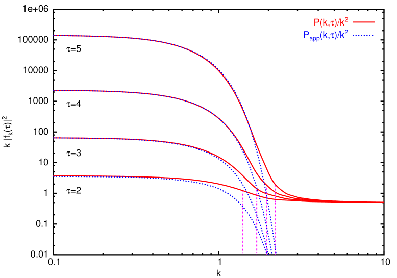
The validity of this approximation can be partially tested in perturbation theory. A first check is the form of the power spectrum (59). We have plotted in Fig. 3 the power spectra $P(k,\tau)$ divided by $k^{2}$, for four values of the normalised time $\tau=2,3,4,5$. Clearly, the power spectra grow in time faster than an exponential, at a very large rate in fact. We take as initial spectrum of the classical field at a given initial time $\tau_{i}$, the exact power spectrum cutoff at $k=\sqrt{\tau_{i}}$. As seen in the figure this encompasses almost all the physically relevant low momentum modes for $\tau_{i}\mathrel{\mathop{\hbox{\lower 2.15277pt\hbox{$\sim$}\kern-8.00003pt\lower-3.01385pt\hbox{$>$}}}}2$.

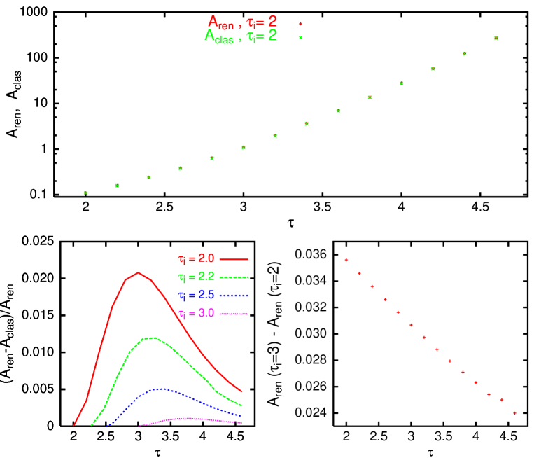
In Fig. 4 we compare, for several values of $\tau_{i}$, $A_{\mbox{\tiny ren}}(\tau,\mu\!=\!\sqrt{\tau_{i}})$ in the fixed-time scheme with $A_{\mbox{\tiny clas}}(\tau,\tau_{i})$, obtained from cutting off the power spectrum, $P(k,\tau_{i})$ in Fig. 3, at $k=\sqrt{\tau_{i}}$. . For $\tau_{i}=2$ the maximal difference between them amounts to 2%, rapidly decreasing as we increase $\tau_{i}$. A direct comparison between the values of $A_{\mbox{\tiny ren}}$ and $A_{\mbox{\tiny clas}}$ for $\tau_{i}=2$ is also shown. The goodness of the approximation performed by truncating the spectrum is clearly evident. We also study the dependence of $A_{\mbox{\tiny ren}}$ on the value of $\tau_{i}$ used for the fixed-time renormalization scheme. We plot the difference between $A_{\mbox{\tiny ren}}$ defined at $\tau_{i}=2$ and $\tau_{i}=3$. As it should, it is of the form $a+b\tau$ and it remains very small in all the range of times we are interested in.

Figure 4: Top: Comparison between $A_{\mbox{\tiny ren}}(\tau,\mu\!=\!\sqrt{\tau_{i}})$, Eqs. (63) and (64), and $A_{\mbox{\tiny clas}}(\tau,\tau_{i})$, the approximation obtained by truncating the spectrum at $\mu=\sqrt{\tau_{i}}$. Bottom: Left: Relative error induced by truncating the spectrum at $\mu=\sqrt{\tau_{i}}$, as a function of $\tau_{i}$. Right: Difference between two choices of the initial time $\tau_{i}$ for the fixed-time renormalization scheme, Eqs. (63) and (64).

It is easy to estimate the time $\tau_{\rm sb}$ when symmetry breaking is expected and the amplification of modes ceases to take place. We can estimate the time of symmetry breaking $\tau_{\rm sb}$ by equating

$$\langle|\phi|^{2}(\tau_{\rm sb})\rangle\equiv M^{2}\,N_{c}A_{\mbox{\tiny ren}}(\tau_{\rm sb},\mu=\sqrt{\tau_{i}})=v^{2}\equiv N_{c}\,v_{0}^{2}\,.$$ (66)

We have just described how for $\tau_{i}\mathrel{\mathop{\hbox{\lower 2.15277pt\hbox{$\sim$}\kern-8.00003pt\lower-3.01385pt\hbox{$>$}}}}2$ a very good approximation for $A_{\mbox{\tiny ren}}$, in the fixed-time subtraction scheme, is obtained by just truncating the power spectrum at $\mu^{2}=\tau_{i}$. We can thus approximate the above expression for the vev by

$$\langle|\phi|^{2}\rangle\equiv{M^{2}\,N_{c}\over 2\pi^{2}}\int_{0}^{\sqrt{\tau}_{i}}dk\,k^{3}\,|f_{k}|^{2}=v^{2}$$ (67)

which can be rewritten as

$$p(\tau_{\rm sb})\simeq\int_{0}^{\sqrt{\tau_{i}}}{dk\over k}\,P(k,\tau_{\rm sb})={2\pi^{2}\over\lambda\,N_{c}\,(2V)^{2/3}}\equiv{2\pi^{2}\over\lambda_{0}\,(2V)^{2/3}}$$ (68)

This can be computed exactly using (43) but to give an analytic estimate of its dependence on the parameters, we will use an approximation to the classical power spectrum (59). In the region of quasi-classical modes it is very well described by,

$$P_{\rm app}(k,\tau)=A(\tau)\,k^{2}\,e^{-B(\tau)\,k^{2}}\,,\hskip 14.22636pt$$ (69)

$$A(\tau)=A_{0}\,{\rm Bi}^{2}(\tau)\,,\hskip 28.45274ptB(\tau)=2\sqrt{\tau}-2\,,$$ (70)

which can be obtained from $|f_{k}|^{2}\simeq\,|C_{1}(k)|^{2}\,|{\rm Bi}|^{2}(z)$, where

$${\displaystyle k\,|C_{1}(k)|^{2}\simeq{\pi^{2}(1/3)^{2/3}\over 2\,\Gamma^{2}(1/3)}\Big{(}1+2k^{2}+{\cal O}(k^{4})\Big{)}\ \simeq\ A_{0}\,e^{2k^{2}}}\,,$$ (71)

$${\displaystyle\exp\Big{(}{4\over 3}z^{3/2}\Big{)}=\exp\Big{(}{4\over 3}\tau^{3/2}-2\sqrt{\tau}\,k^{2}+{\cal O}(k^{4})\Big{)}}\,.$$ (72)

We have plotted $P_{\rm app}(k,\tau)$ together with the exact spectrum in Fig. 3. We can see that it is an excellent approximation to the classical power spectrum, in the region of interest. Using $P_{\rm app}(k,\tau)$ to estimate (68) gives the condition

$$p(\tau_{\rm sb})={2\pi^{2}\over\lambda_{0}\,(2V)^{2/3}}\simeq\int{dk\over k}\,P_{\rm app}(k,\tau_{\rm sb})={A(\tau_{\rm sb})\over 2B(\tau_{\rm sb})}\,,$$ (73)

We have evaluated this function $p(\tau_{\rm sb})$ numerically and found an excellent fit to it, in the range $\tau\geq 1$, as, for $N_{c}=4$,

$$\ln\,p(\tau_{\rm sb})=-3.5+[8+\tau_{\rm sb}^{3.23}]^{1/2}\,,$$ (74)

which gives directly the time of symmetry breaking in units of $m^{-1}$,

$$mt_{\rm sb}=(2V)^{-1/3}\left[\Big{(}3.5+\ln{2\pi^{2}\over\lambda_{0}(2V)^{2/3}}\Big{)}^{2}-8\right]^{0.31}\,.$$ (75)

We can use this compact expression to estimate the time of symmetry breaking for any coupling $\lambda$ and any inflaton velocity $V$ at the bifurcation. For example, for $\lambda_{0}=0.11$ and $V=0.003$, we find $\tau_{\rm sb}=4.6$ and $mt_{\rm sb}=25.3$, which agrees very well with numerical (lattice) simulations performed for those values of the parameters.

Note that, as mentioned before, the dependence of $\tau_{\rm sb}$ with the parameters $\lambda\equiv\lambda_{0}/N_{c}$ and $V$ is very mild. In the whole range of parameters, $\lambda_{0}\,(2V)^{2/3}\in[10^{-8},\ 1]$, the normalised time of symmetry breaking only varies within the range $\tau_{\rm sb}=5\pm 2$. Some particular examples can be found in Table 1.

Table 1: The time scales of symmetry breaking and the onset of the non-linear stage for different model parameters. The coupling depends on the number of components of the Higgs field as $\lambda_{0}=N_{c}\lambda$.

$V$	$\lambda_{0}$	$\tau_{\rm nl}$	$mt_{\rm nl}$	$\tau_{\rm sb}$	$mt_{\rm sb}$
0.003	0.11	2.78	15.3	4.6	25.3
0.003	0.01	3.76	20.7	5.2	28.5
0.0003	0.001	4.01	47.5	6.0	71.3
0.00002	0.0001	4.82	141.	6.8	200.

VI Non-linear evolution of the classical system

In the previous sections we have argued that the first stages of the quantum evolution of the system (when the non-linear self-coupling of the Higgs is negligible) drive the system into a state with highly populated low momentum modes. The evolution of this state can be accounted for by the evolution of a classical (approximately gaussian) random field. This justifies the main assumption of this and remaining sections, namely that the subsequent non-linear dynamics of the system is determined by the classical evolution of this field. This evolution is deterministic and the random character appears in the initial values of the field at time $\tau=\tau_{i}$. These initial conditions are determined by the exact gaussian quantum evolution of the system studied in the previous section. Thus, the initial Higgs field is chosen gaussian, an approximation which can be tested by probing the sensitivity of our results to the value of $\tau_{i}$. As we will see this works very well within the appropriate range of initial times. Some statistical properties of this initial gaussian random field can be studied analytically. This is done in section 6.1. These properties extend to times during which the evolution is essentially linear and the field remains approximately gaussian. A full non-perturbative treatment of the dynamics can only be done by numerical methods. We have actually carried this step by lattice simulations. This is described in section 6.2 where a full account of the methodology and the checks performed to show cut-off independence is described. Results will be presented in the next section

VI.1 Peaks of the Higgs spatial distribution

The statistics of the Higgs spatial distribution can be determined from the gaussian fluctuations that are used to build it up. A detailed description can be found in Ref. BBKS for the case of the gaussian density field responsible for galaxy formation. In fact, the spatial distribution and subsequent dynamical behaviour of the Higgs field at the initial stages of symmetry breaking turns out to be not that different from that of both the linear and non-linear growth of the cosmological density field (also built up from the gaussian random fields of cosmological perturbations), except in the dynamics of gravitational collapse of the latter.

The fact that the quantum fluctuations of the Higgs give rise to a classical gaussian random field, allows us to study the statistical properties of this field in terms of a single function, the two-point correlation function in Fourier space (i.e. the power spectrum), whose approximate expression can be found in (69). This quantity allows the computation of several related quantities that characterise a gaussian random field, e.g. the spatial correlation function, the density of peaks above a certain threshold, the shape of the highest peaks, etc.

The first quantity that we can compute is the spatial correlation function, defined as the two-point correlation function between two points separated by a distance $r$,

$$\xi(r,\tau) \equiv \left\langle\phi(r,\tau)\phi(0,\tau)\right\rangle={M^{2}\,N_{c}\over 2\pi^{2}}\int_{0}^{\infty}{dk\over k}\,P_{\rm app}(k,\tau)\,{\sin\,kr\over kr}$$ (76)

$$\simeq {M^{2}\,N_{c}\over 2\pi^{2}}{A(\tau)\over r}\int_{0}^{\infty}dk\,e^{-B(\tau)k^{2}}\,\sin\,kr$$

$$= {M^{2}\,N_{c}\over 2\pi^{2}}{A(\tau)\sqrt{\pi}\over r\,2B^{1/2}(\tau)}\,\exp\Big{(}\!-{r^{2}\over 4B(\tau)}\Big{)}\,{\rm erfi}\Big{(}{r\over 2B^{1/2}(\tau)}\Big{)}\,,$$

where $\ {\rm erfi}(x)$ is the imaginary error function AS . This correlation function determines the average size of the lumps, $\xi_{0}$,

$$\xi_{0}\simeq 2B^{1/2}(\tau)\simeq 2\sqrt{2\sqrt{\tau}-2}\,,$$ (77)

as a function of normalised time $\tau$. Note that the time dependence of the correlation length is different than for a quench symmetry breaking. While in the latter case, the correlation length grows like $\xi_{0}\sim 2\sqrt{\tau}$, in our case, it grows like $\xi_{0}\sim 2\sqrt{2}\,\tau^{1/4}$ for “large” $\tau$ (still in the linear regime). This introduces some slight differences in the behaviour of the field at symmetry breaking.

We can then compute from (76) the time-dependent dispersion

$$\sigma(\tau)\equiv\xi^{1/2}(0,\tau)=\phi_{\rm rms}(\tau)={M\,\sqrt{N_{c}}\over\sqrt{2}\,\pi}\,p^{1/2}(\tau)\,,$$ (78)

which is nothing but the root mean square value of the Higgs field.

Another quantity which is very useful to characterise the field distribution is the number density of peaks of the field above a certain threshold $\phi_{c}$, see Ref. BBKS ; HGW

$$n_{\rm peak}(\tau)={1\over 4\pi^{2}}\left({-\xi^{\prime\prime}(0,\tau)\over\xi(0,\tau)}\right)^{3/2}(\nu^{2}-1)\,\exp(-\nu^{2}/2)\,,$$ (79)

$${-\xi^{\prime\prime}(0,\tau)\over\xi(0,\tau)}={\langle k^{2}\rangle\over 3}={\int(dk/k)P(k,\tau)k^{2}\over 3\int(dk/k)P(k,\tau)}\,,\hskip 28.45274pt$$ (80)

where $\nu={\phi_{c}\over\sigma(\tau)}>1$. In our case, the number density of high peaks is given by

$$n_{\rm peak}(\tau) = {2\over 3\sqrt{3}\,\pi^{2}}\,{1\over r_{0}^{3}(\tau)}\,(\nu^{2}-1)\,\exp(-\nu^{2}/2)\,,$$ (81)

$$\nu(\tau) = {\phi_{c}\over v}\,{\sqrt{2}\,\pi\over(2V)^{1/3}\sqrt{\lambda}_{0}}\,p^{-1/2}(\tau)\,.$$ (82)

We have evaluated this function for the parameters $\lambda=0.11/4$ and $V=0.003$, at various times and compared with our lattice simulations (for different volumes $V=(2\pi/p_{\rm min})^{3}$ and lattice spacings $a$). The results are very encouraging. If we multiply this density of peaks by the actual volume of the simulations, we find indeed just a few peaks above e.g. $\phi_{c}=0.02v$, at the time of symmetry breaking.

In fact, we can compute not only the probability per unit volume to find a peak in the distribution of the Higgs field, but also their radial profile BBKS ,

$$\rho(r,\tau) = {M\,\sqrt{N_{c}}\over\sqrt{2}\,\pi}\int_{0}^{\infty}{dk\over k}\,P^{1/2}_{\rm reg}(k,\tau)\,{\sin\,kr\over kr}$$ (83)

$$\simeq {M\,\sqrt{N_{c}}A^{1/2}(\tau)\over\sqrt{2}\,\pi\,r}\int_{0}^{\infty}{dk\over k}\,e^{-{B(\tau)\over 2}k^{2}}\,\sin\,kr$$

$$= {M\,\sqrt{N_{c}}A^{1/2}(\tau)\over 2\sqrt{2}\,r}\,{\rm erf}\Big{(}{r\over\sqrt{2B(\tau)}}\Big{)}\,,$$

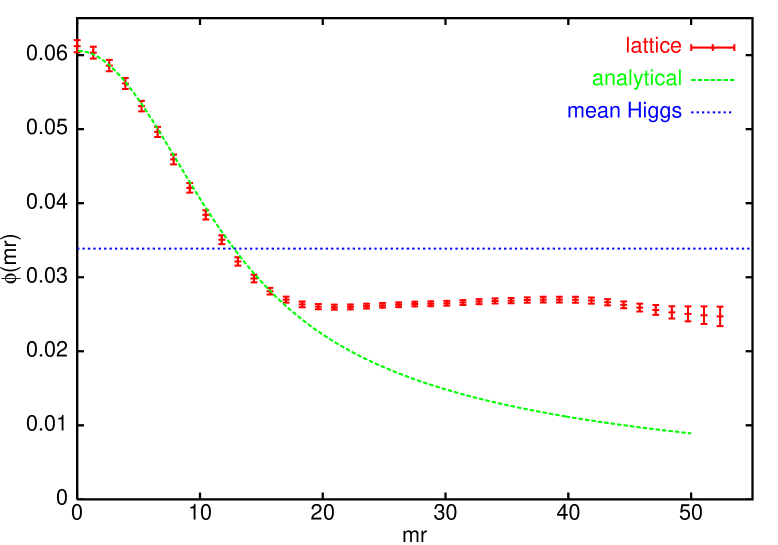
where $\ {\rm erf}(x)$ is the error function AS . We have plotted this profile function in terms of the radial coordinate, together with the lattice results in Fig. 5, for $\lambda=0.11/4$ and $V=0.003$, at time $\tau=2.54$, corresponding to $mt=14$, well before symmetry breaking, which occurs at $mt_{\rm sb}\simeq 26$.

Figure 5: The radial profile of the Higgs peak for $\lambda=0.11/4$ and $V=0.003$, at time $\tau=2.54$, corresponding to $mt=14$, obtained with our lattice simulation (with error bars, from averaging over several realizations), and compared with the analytical result (83). We have also included the rms Higgs value (78) at that time. Note that we are still in the linear regime, where (83) gives a very good approximation. The higher tail corresponds to an averaging out of several lower peaks.

VI.2 Lattice simulations

The previous analysis falls short of addressing the most important aspects of symmetry breaking after hybrid inflation since the main effect is non-perturbative, see Ref. GBKLT . As discussed we will incorporate these effects by performing classical real-time numerical simulations in the lattice. Generically this classical approximation would fail to reproduce the relevant physics but we have just argued that this is indeed the correct approximation for the infrared modes of the Higgs at the time of symmetry breaking.

The usual procedure FT is to take as initial conditions for the lattice simulations gaussian random fields given by the distribution (34) with vacuum initial amplitudes corresponding to Eqs. (17), (18). We would like to stress here that the correct description of the quantum linear system in terms of a gaussian random field requires the use of two independent gaussian variables, as indicated in (34). One of them, $y$ in (34), describes field fluctuations with dispersion $|f_{k}|^{2}$ and a random phase. The other, $\bar{p}$, with dispersion $(4\,|f_{k}(\tau)|^{2})^{-1}$ and a random phase, allows to define the conjugate momentum through, see Appendix B,

$$p=\bar{p}+{F_{k}(\tau)\over|f_{k}(\tau)|^{2}}\,y\,.$$ (84)

Notice that this prescription is valid in order to give initial conditions at any time during the evolution before non-linearities set in. In particular, as described in section V, we propose to take as starting point for the lattice simulations the above gaussian ensemble at a fixed time sufficiently advanced to guarantee that a large fraction of modes have become classical, but well before the time when non linearities become relevant, in a similar spirit as that in Ref. Smit . This has the advantage of allowing a clear separation between infrared (classical) modes which evolve classically and ultraviolet (quantum ) modes that will be absorbed in the renormalization of the constants of the theory. From the previous analysis, see Fig. 2 and the discussion after Eq. (75), a good choice for the matching time in a wide range of model parameters seems to be $\tau_{i}\simeq 2$. See the discussion in the next section about the onset of the non-linear regime.

Therefore, we propose the following as initial conditions in our lattice simulations. At a fixed time $\tau_{i}$ previous to symmetry breaking:

• Put to zero all the modes that have not become classical at $\tau_{i}$. This includes all the modes of the inflaton but the homogeneous zero mode, and all large momentum modes of the Higgs with $k>\sqrt{\tau_{i}}$ (replacing the hard cutoff at $\sqrt{\tau_{i}}$ by the approximate power spectrum in (69), which strongly dumps ultraviolet modes, does not significantly change the results even at a quantitative level).

• Set the homogeneous zero mode of the inflaton to $\chi/\chi_{c}=1-Vm\,t_{i}$ with conjugate momentum $\dot{\chi}/\chi_{c}=-Vm$.

• For the Higgs fluctuations, each Fourier component, with momentum $|k|\leq\sqrt{\tau_{i}}$, has an amplitude $|\phi_{k}|$ randomly generated according to the Rayleigh distribution:

  $$P(|\phi_{k}|)\,d|\phi_{k}|\,d\theta_{k}=\exp\Big{(}\!-{|\phi_{k}|^{2}\over\sigma_{k}^{2}}\Big{)}\,{d|\phi_{k}|^{2}\over\sigma_{k}^{2}}\,{d\theta_{k}\over 2\pi}\,,$$ (85)

  with dispersion given by $\sigma_{k}^{2}=|f_{k}|^{2}=k^{-3}\,P(k,\tau_{i})$, and a uniform random phase $\theta_{k}\in[0,2\pi]$. The conjugate momentum $g_{k}=i\phi^{\prime}_{k}$ is uniquely determined once $\phi_{k}$ is known, through the relation

  $$\phi_{k}^{\prime}={F_{k}(\tau_{i})\over|f_{k}(\tau_{i})|^{2}}\ \phi_{k},$$ (86)

  with $f_{k}(\tau_{i})$ and $F_{k}(\tau_{i})$ given by Eqs. (43) and (26), respectively, at $\tau=\tau_{i}$. This corresponds to the classical limit of (84), an approximation that is well justified for $\tau_{i}\mathrel{\mathop{\hbox{\lower 2.15277pt\hbox{$\sim$}\kern-8.00003pt\lower-3.01385pt\hbox{$>$}}}}2$, see Appendix B.

• Take the masses and couplings used in the simulation as the physical renormalised ones in the fixed-time subtraction prescription.

Figure 6: The time evolution of $\langle|\phi|\rangle$, $\langle\chi\rangle$ and energies (normalised to the initial one) for $\lambda\!=\!0.11/4$ and $V\!=\!0.003$, obtained with our lattice simulation. Left: for different choices of $mt_{i}$, the time for matching the quantum evolution to the classical lattice simulations. Right: for different values of the lattice spacing $ma=0.98,1.31,1.96$.

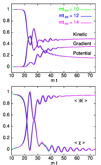
As long as the time chosen for initialisation is sufficiently advanced that a large fraction of modes have become classical, we hope that most of the physics responsible for symmetry breaking will be included in the simulations. How advanced it has to be in a concrete realization can be tested by studying in which range the time evolution is insensitive to the choice of $\tau_{i}$. This provides also a check of the validity of our approach. The result of such a test is presented in Fig. 6. We compare the time evolution of $\langle|\phi|\rangle$, $\langle\chi\rangle$ and the average kinetic, gradient and potential energies obtained from setting the initial conditions at $mt_{i}=10,12,14$ ($\tau_{i}=1.81,2.18,2.54$) for $\lambda=0.11/4$ and $V=0.003$. The agreement is excellent, corroborating our estimate that for $\tau_{i}\simeq 2$ all the basic relevant modes driving symmetry breaking have already become classical and thereafter the evolution is well described by our lattice classical simulations.

All the lattice results presented in this paper have been obtained for a SU(2) Higgs doublet coupled to the inflaton with coupling $g^{2}=2\lambda=0.22/4$, and inflaton velocity $V=0.003$. Due to the finite volume, the momentum $k$ is discretised in units of a minimal momentum given by $p_{\rm min}=2\pi/L$, with $L=Na$, where $N$ is the number of lattice points, and $a$ the lattice spacing. Our simulations have been performed in lattices of sizes $32^{3}$, $48^{3}$ and $64^{3}$ with physical volumes determined by $p_{\rm min}=0.1m,\ 0.075m$ and $0.05m$ and lattice spacings varying from $ma\simeq 1$ to $ma\simeq 2$. The choice of lattice volumes and lattice spacings has been performed such as to avoid lattice spacing and finite volume dependence of the lattice results. Notice that the minimal momentum has to be small enough that a sufficiently large number of classical momenta with $k\mathrel{\mathop{\hbox{\lower 2.15277pt\hbox{$\sim$}\kern-8.00003pt\lower-3.01385pt\hbox{$<$}}}}1$ is taken into account. We have found that for $p_{\rm min}\leq 0.1m$ this is indeed the case and no significant volume dependence is observed.

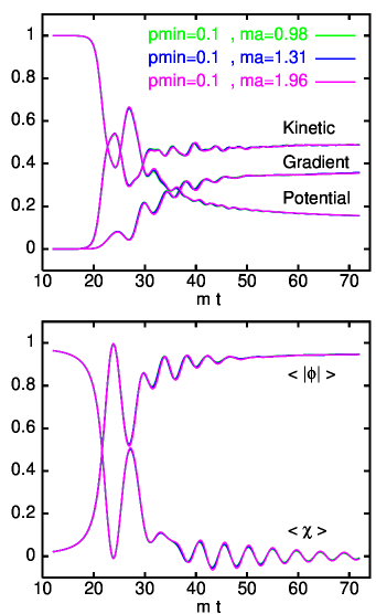
A further essential test of our approach is that it succeeds in taming ultraviolet divergences. On the lattice there is a maximal momentum determined by the lattice cutoff through $p_{\rm max}=2\pi/a$. Naturally, re-scattering and back-reaction will populate the high momentum modes at and after symmetry breaking This is certainly a physical effect but if the lattice cutoff is not chosen large enough population of the high momentum modes is artificially induced by cutoff effects. The lattice cutoff should then be chosen such as to avoid that this takes place before the relevant dynamics of symmetry breaking. A reasonable value for our choice of parameters is $ma<2$, as can be seen from Fig. 6, where we compare the time evolution of $\langle|\phi|\rangle$, $\langle\chi\rangle$ and average energies for several values of the lattice cutoff $ma=0.98,1.31,1.96$. No significant lattice spacing dependence is observed here, while it becomes clearly appreciable for $ma>3$. Details of the simulations and further results will be presented elsewhere. These lattice simulations will allow us to test the next stage, the non-linear approach to symmetry breaking.

VII Results of the non-linear analysis and “bubble” formation

Figure 7: Snapshots of the growth of the Higgs peak in a full non-linear lattice simulation, for $\lambda=0.11/4$ and $V=0.003$. Plotted is the value of the Higgs amplitude $\phi$ in the plane $(x,\ y)$, where the $z$-coordinate is that of the highest peak. Note that several peaks appear in the simulation. Here we show the first stages of the evolution, where the highest peak invaginates and forms what we call the “bubble”.

Figure 8: Same as in Fig. 7. Here we show the late stages, in which gradients arise from collisions of bubbles and the symmetry is broken, i.e. $\phi\simeq 1$.

In the previous sections we have developed a formalism to describe the linear growth of the Higgs quantum fluctuations and their conversion into a classical gaussian random field. As we have argued, in the linear regime there is only the homogeneous mode of the inflaton, $\langle\chi/\chi_{c}\rangle=1-Vm(t-t_{c})$, which induces a negative mass squared (5) for the Higgs, and thus its spinodal instability towards the true vacuum. The quick growth of the quantum fluctuations generates a gaussian random field with correlation function (76), and a rms field value, see (78),

$$\phi(\tau)\equiv{\phi_{\rm rms}\over v}={(2V)^{1/3}\sqrt{\lambda N_{c}}\over\sqrt{2}\,\pi}\,p^{1/2}(\tau)\,,$$ (87)

where $p(\tau)$ is given by (68). Eventually, the mean field $\phi$ will become large and will approach the vev of its potential, thus breaking the symmetry. Before that happens, its coupling to the inflaton will induce a back-reaction on the homogeneous mode of the inflaton, $\chi$, which will start to deviate from the linear regime described above. At this stage the non-perturbative evolution can be studied by numerically solving the coupled classical equations of motion for the inflaton and Higgs:

$${\displaystyle\ddot{\phi}^{a}({\bf x},t)-\nabla^{2}\phi^{a}({\bf x},t)+(|\phi|^{2}({\bf x},t)+\chi^{2}({\bf x},t)-1)\,\phi^{a}({\bf x},t)=0\,,}$$ (88)

$${\displaystyle\ddot{\chi}({\bf x},t)-\nabla^{2}\chi({\bf x},t)+{g^{2}\over\lambda}|\phi|^{2}({\bf x},t)\,\chi({\bf x},t)=0\,,}\hskip 71.13188pt$$ (89)

with gaussian initial conditions as described in the previous sections. In this section we will present the results of our numerical simulations and give an approximate analytic understanding of how symmetry breaking takes place.

Although the initial conditions are random, as a result of the non-linear dynamics many of the qualitative features of the evolution are fairly universal, although quantitatively different configurations differ by small shifts in the origin of times as well as spatially random positions for the center of the peaks. Therefore, we prefer to illustrate our analytic formulas by comparing with the results of a typical lattice configuration, e.g. the one displayed in Figs. 6-8.

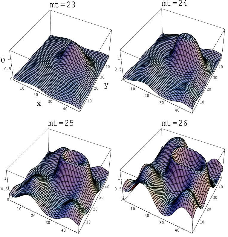
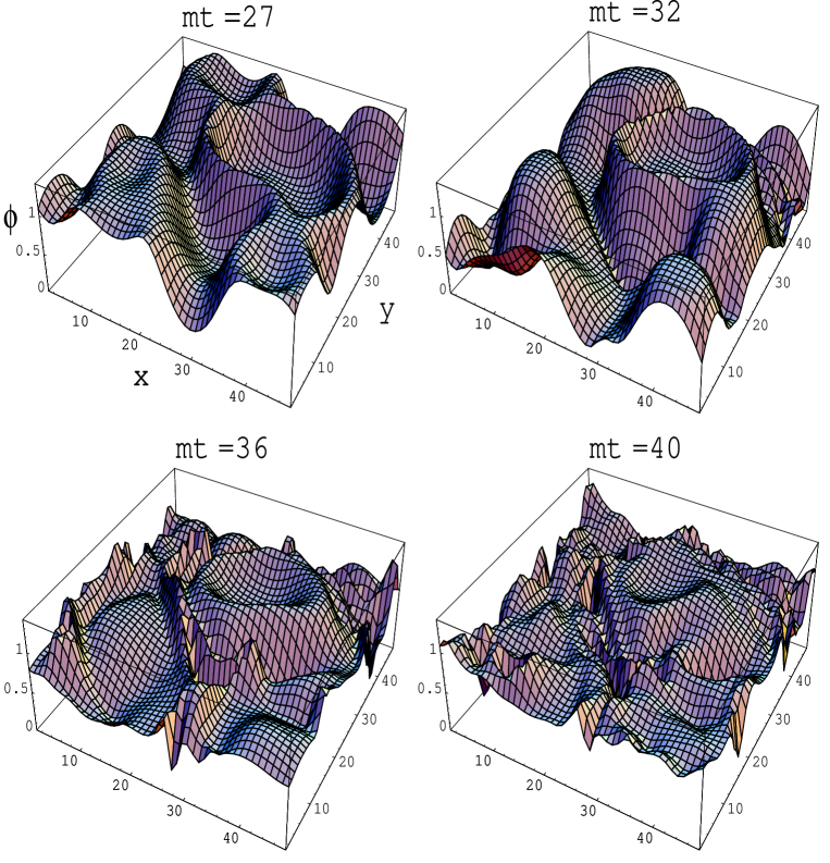
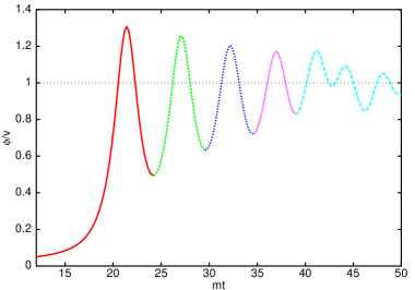
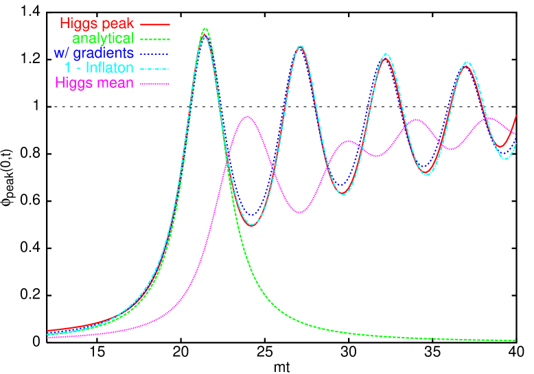
Symmetry breaking in our model is not at all a homogeneous process. Already in the linear regime, the Higgs field evolves by developing lumps in space that grow with time, see (83) and Fig. 5. The classical evolution of the Higgs’ lumps, once non-linearities become relevant, can be followed in Figures 7 and 8 where we show some snapshots of the growth of the Higgs’ peaks from the first stages of the evolution, $mt=23$, till $mt=40$ above which full symmetry breaking takes place and the mean Higgs field approaches the vev. As can be seen from the figures, the peak of the largest Higgs’ lump is the first to break the symmetry, i.e. to reach $|\phi|=v$, and soon after the center of the lump invaginates, creating an approximately spherically symmetric “bubble”, with “ridges” that remain above $|\phi|=v$. Finally, neighbouring bubbles collide and the symmetry gets fully broken through the generation of higher momentum modes. In Fig. 9 we show the behaviour of $|\phi({\bf x},t)|$ at the center of the highest Higgs lump. It oscillates around $|\phi|=v$ with an amplitude that is dumped in time. Oscillations remain coherent giving rise to concentric bubbles, until the time when bubble collisions break the symmetry.

Figure 9: Left: The time evolution of the modulus of the Higgs, at the location of the highest Higgs peak. Plotted is the Higgs modulus $\phi/v$ as a function of time. Note the effect of bubble collisions on the Higgs oscillations after $mt=40$. Right: Collinear evolution of the inflaton and the Higgs at the location of the highest Higgs peak. Note that the inflaton and Higgs satisfy $\phi=1-\chi$ to very good accuracy, until rather late, when “bubbles” start to collide.

It is possible to get an analytic understanding on how this non-linear process takes place before bubbles start to collide. For the problem we are considering, we can rewrite the components of the Higgs field as $\phi^{a}\equiv\phi\,\hat{n}_{a}$ (we will use from now on the symbol $\phi$ to denote the modulus of the Higgs) while $\Omega=\hat{n}\cdot\sigma\in$ SU(2) is an element of the gauge group, with $\sigma=(1\!{\rm l},\ i\vec{\tau})$ with $\tau_{a}$ the Pauli matrices. With this the equations of motion for the coupled inflaton Higgs field can be rewritten as

$${\displaystyle\ddot{\phi}({\bf x},t)-\nabla^{2}\phi({\bf x},t)+(\phi^{2}+\chi^{2}-1)\,\phi-\,|\partial_{\mu}\hat{n}|^{2}\,\phi=0\,,}$$ (90)

$${\displaystyle\partial^{\mu}(\phi^{2}\,\partial_{\mu}\hat{n})=-\hat{n}\,\,\phi^{2}\,|\partial_{\mu}\hat{n}|^{2}}\,,$$ (91)

$${\displaystyle\ddot{\chi}({\bf x},t)-\nabla^{2}\chi({\bf x},t)+{g^{2}\over\lambda}\phi^{2}\,\chi=0\,,}$$ (92)

where dots and $\nabla$ denote derivatives with respect to $mt$ and $m{\bf x}$ respectively, and the homogeneous modes have been normalised to their vevs, $\phi/v\to\phi$ and $\chi/\chi_{c}\to\chi$.

Figure 10: The histogram of field values for the Higgs modulus $\phi$ and the co-inflaton $1-\chi$. Note that soon after the initial condition and the subsequent non-linear evolution, the two coincide very precisely. Note that a few oscillations can be observed during symmetry breaking, i.e. during times $mt=22-30$.

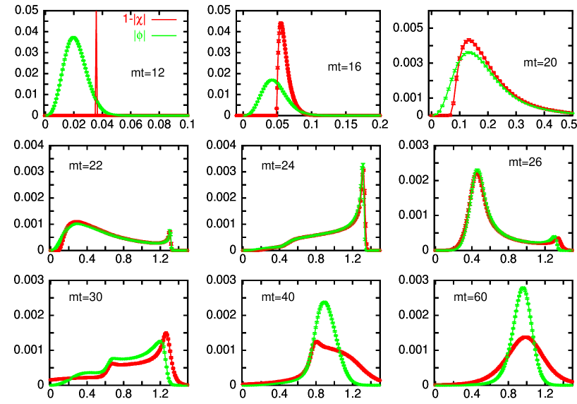
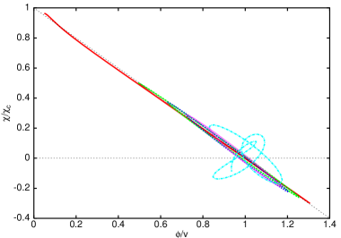
We can take advantage of the fact that, for $g^{2}=2\lambda$, a solution to the set of coupled equations of motion is given by $\phi({\bf x},t)=1-\chi({\bf x},t)$ BGK ; GBKLT and $\partial^{\mu}(\phi^{2}\,\partial_{\mu}\hat{n})=0$. Numerical results corroborate that this is very approximately the solution soon after non-linearities set in. In Figure 9 we show, for our model with parameters $V=0.003$ and $\lambda=0.11/4$, $\phi$ versus $1-\chi$ at the location of the highest Higgs lump. Comparing with Figure 9 we can follow how the Higgs and inflaton evolve colinearly during all the time of coherent oscillations of the peak. In Fig. 10 we show the distribution of field values as a function of time, in the time interval between $mt=12$ and $mt=60$, where most of the action takes place. During most of the non-linear initial stage, through symmetry breaking and until bubbles collide we have: $\phi({\bf x},t)=1-\chi({\bf x},t),\ \forall{\bf x}$ .

Figure 11: The time evolution of the Higgs peak ($r=0$) and the Higgs rms value, obtained with our lattice simulations, as compared with the analytical result (97), and the numerical solution of equation (100), which includes the gradient terms. Also shown is the comparison between the Higgs and the inflaton evolution, i.e. $\phi(t)$ and $1-\chi(t)$.

Figure 12: The time evolution of the Higgs radial profile around the highest peak, obtained with our lattice simulation (points), as compared with the numerical solution of the partial differential equation (lines). It is surprising how well the formation of the bubble is reproduced with the simple assumption of homogeneity around the peak of the bubble. Of course, the peak solution does not take into account the presence of secondary bubbles, that appear in the lattice simulation at $r\sim 30$.

During the time that inflaton and Higgs evolve colinearly, the system can be seen as that of a single field with a modified potential $\bar{V}(\phi)$, with the minimum at $\phi=1$.

$${\cal S} = {3\over 2}\,\int d^{3}{\bf x}\,dt\left[{1\over 2}(\partial_{\mu}\phi)^{2}-\bar{V}(\phi)\right]\,,$$ (93)

$$\bar{V}(\phi)={1\over 6}\Big{(}1-4\phi^{3}+3\phi^{4}\Big{)}\,.$$

The equation of motion of the scalar field $\phi$ becomes a non-linear partial differential equation

$$\ddot{\phi}({\bf x},t)-\nabla^{2}\phi({\bf x},t)-2\phi^{2}({\bf x},t)+2\phi^{3}({\bf x},t)=0\,.$$ (94)

If the gradient terms are much smaller than the non-linear ones, we can as a first approximation neglect them leading to

$$\ddot{\phi}(t)-2\phi^{2}(1-\phi)=0\,,$$ (95)

which leads to a conserved energy $E=E_{0}+{1\over 6}$ with

$$E_{0}\equiv{1\over 2}\Big{(}\dot{\phi}^{2}(t)-\phi^{3}({4\over 3}-\phi)\Big{)}\,.$$ (96)

A solution with $E_{0}=0$, a very good approximation taking into account that initially both the field and its derivative are very small, is given by

$$\phi(t)=1-\chi(t)={12\over 9+4[mt-mt_{\rm max}]^{2}}\,,$$ (97)

with $t_{\rm max}$ the time at which the field reaches its maximum value: $\phi(t_{\rm max})={4\over 3}$. This time can be rewritten in terms of the value of the field at any other time $t_{\rm nl}$ through

$$mt_{\rm max}=mt_{\rm nl}+\sqrt{{3\over\phi_{0}}-{9\over 4}}\,.$$ (98)

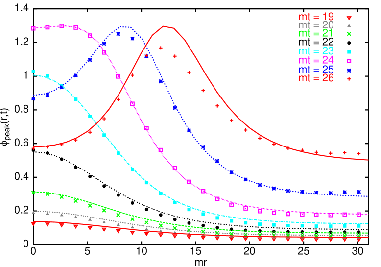
In particular, at every point ${\bf x}$, we can take $\phi_{0}$ as the “initial” value of the Higgs field. This is given by the profile of the lump in the linear approximation, Eq. (83), at a time $t_{\rm nl}$ at which the evolution becomes non-linear and we can no longer ignore its higher order interactions. In Fig. 11 we show again the non-linear growth of the Higgs field at the top of the largest peak in the simulation, and compare it with the analytical solution (97). The agreement is very good during the first oscillation although (97) cannot reproduce the subsequent ones. At these stage we can already understand how the spherical bubbles arise. Take the spherically symmetric peak profile (83) at the non-linear time $t_{\rm nl}$ and let each point ${\bf x}$ evolve like (97). Points with higher value of $\phi_{0}(t_{\rm nl})$ will reach first the maximum value ($\phi_{\rm max}={4\over 3}$) and then decrease. This generates a spherical wave that propagates from the center of the lump to infinity. The production of bubbles associated with symmetry breaking were first described in Ref. GBKLT for the model $\lambda\phi^{3}$, which is analogous to our reduced model. The subsequent evolution is of course different, due to the presence of the inflaton field.

We can evaluate the non-linear time, $t_{\rm nl}$, by equating

$$\chi(\tau_{\rm nl})=1-{1\over 2}(2V)^{2/3}\tau_{\rm nl}=1-\phi(\tau_{\rm nl})\,.$$

Using (87) and (74), we can find the nonlinear time $\tau_{\rm nl}$ as the solution of the transcendental equation

$$\tau=\left[\Big{(}3.5+2\,\ln{\pi(2V)^{1/3}\tau\over\sqrt{2\lambda N_{c}}}\Big{)}^{2}-8\right]^{0.31}\,.$$ (99)

For the values of parameters chosen, $\lambda=0.11/4$ and $V=0.003$, we find $mt_{\rm nl}=15.3$ and $\phi_{0}=0.1$. That is, soon after the Higgs field becomes non-linear, it ceases to grow exponentially like (87), and starts to grow like (97), which has a peak at $mt_{s}\simeq 23\mathrel{\mathop{\hbox{\lower 2.15277pt\hbox{$\sim$}\kern-8.00003pt\lower-3.01385pt\hbox{$<$}}}}mt_{\rm sb}\simeq 26$, see Fig. 11. This corresponds to a time slightly earlier that the time of symmetry breaking. This is of course natural since, as we have described, the Higgs field has an inhomogeneous spatial distribution. The mean field (coarse-grained over a horizon-sized volume) is much lower than a typical peak of the field. The top of the peak follows very approximately the homogeneous equation (95), with solution (97). High peaks will reach the symmetry breaking vev much earlier than the mean field, and will oscillate around the vev with a much larger amplitude that the average (coarse-grained) field.

Obviously, the phenomenological damping of oscillations that we have described has to arise from the gradient terms which we have neglected. Hence, we will improve our approximation by keeping these terms, but assuming spherical symmetry ($\phi({\bf x},t)\rightarrow\phi(r,t)$) around the center of the lump ($r=0$). Our lattice data support the approximate validity of this assumption. This will allow us to track the time-evolution of the lump profile as it develops into bubbles. The two-dimensional partial differential equation for $\phi(r,t)$ becomes:

$$\ddot{\phi}(r,t)-\phi^{\prime\prime}(r,t)-{2\over r}\phi^{\prime}(r,t)-2\phi^{2}(r,t)+2\phi^{3}(r,t)=0\,.$$ (100)

We have solved this equation numerically. The initial condition was fixed at a time $mt_{\rm nl}$ when the profile matches expression (83). In order to compare with the non-linear lattice simulations, we added by hand a tail a long distances , to match the lattice initial conditions, see Fig. 5. To fix a unique solution, one has also to fix $\dot{\phi}(r,t_{\rm nl})$. Choosing this derivative equal to zero we have obtained the shape $\phi(r,t)$ for all times in the region of interest. In Fig. 12 we present the result of the comparison of these results with those obtained from the full 4D lattice real-time equations of motion. The general shape is quite properly reproduced. Furthermore, the oscillations of the peak height are also recovered, see Fig. 11.

As a last remark, note that the bubbles that appear here are not vacuum bubbles like those produced in a first order phase transition, since the interior of them is not in the true vacuum. Furthermore, we note also that the ridges of the bubbles are moving very fast and presumably subsequent collisions between bubbles formed at different space-time points are highly relativistic, and may be responsible for a large density of gravitational waves, which could be seen in LISA.

For a typical lattice configuration one can follow the evolution of the Higgs from the formation of the first bubbles to the breaking of the symmetry with the .gif file that can be found in the web page: http://lattice.ft.uam.es/SymBrk/2dHiggs.gif

VIII Conclusions

In this paper we have studied the evolution of a hybrid inflation model from the quantum false vacuum state at the end of inflation to the broken symmetry true vacuum state. A full description of this dynamics amounts to a non-perturbative, non-linear, real-time evolution of the quantum system, which looks a priori like a formidable task. The size of non-linear effects is given by $\lambda\phi^{2}$, where $\lambda$ is the coupling constant and $\phi^{2}$ the square of the typical value of the Higgs field. Since initially $\phi^{2}$ and $\lambda$ are small, it is reasonable to assume that perturbation theory is a good approximation and the dynamics is well approximated by the gaussian Hamiltonian. However, the quantum evolution of this gaussian system, which can be treated exactly, is far from trivial. The complexity results from the negative time-dependent mass-square of low-momentum Higgs modes induced by the coupling to the inflaton. This tachyonic dynamics generates a faster than exponential tachyonic growth of low-lying momentum modes of the Higgs, giving rise to regions where $\lambda\phi^{2}$ is non-negligible and where non-linearities set in. In this paper we have shown that the dynamics of the tachyonic modes is well-described by that of a classical gaussian random field, a result that holds even after including perturbative corrections in the coupling, which are still accessible to exact computation. At this stage important considerations set in through the appearance of ultraviolet divergences. High-momentum modes cannot be neglected but their effect can be absorbed in the value of the couplings of the theory. Here, in addition to the usual standard time-independent renormalization, a renormalization of the initial velocity of the inflaton field is required to get rid of the time-dependent infinities generated at first order in the coupling $\lambda$.

The previous analysis justifies the next stage of the study carried out in this paper, namely the classical non-linear evolution of the resulting classical field. This problem can be addressed numerically by formulating the problem on a spatial lattice and evolving the system according to the classical real-time evolution equations. The initial conditions on the classical field are determined by the previously computed (non-self-interacting) quantum Higgs evolution. Our results are independent of all cut-offs introduced by this numerical procedure: the initial time of the simulation, the lattice-spacing and the finite lattice volume. This, of course, provided they are taken in the appropriate ranges.

The resulting non-linear evolution which drives the system towards symmetry breaking is fairly non-trivial. The inhomogeneous Higgs field distribution has lumps in space whose height grows with time during the approximately linear evolution phase. This growth continues, although at a slower pace, when the non-linear terms become relevant. The behaviour changes again as the highest lumps reach the magnitude of the Higgs vacuum expectation value. Then the lumps evolve into approximately spherically symmetric bubbles which expand at a very high speed. It is important not to confuse these bubbles with those appearing in a first order phase transition which separate two different phases. Our bubbles are rather like spherical shock waves as those appearing in Ref. GBKLT . These stages of the non-linear evolution can be qualitatively and quantitatively understood analytically. The last phase of evolution arises as neighbouring bubbles collide and generate higher momentum modes. This phase is harder to tackle analytically but its early stages, at least, seems relatively safe for our lattice numerical procedure.

In the early stages of evolution our results resemble those obtained for a one component Higgs model in Ref. CPR , as expected from the decoupling of the different components of the Higgs field in the linear regime. At later times, however, the comparison is difficult due to the different nature of the defects in both theories.

The authors are presently studying how the previously described processes might be influenced by the coupling to gauge fields, and its application to the study of physical phenomena such as baryogenesis. We anticipate that there is no essential obstruction for incorporating gauge fields, although the formalism complicates considerably. Furthermore, the numerical evolution including gauge fields does not change substantially the gross features of the picture described here. All this will be the subject of a future publication.

Appendix A The formalism of squeezed states

In this appendix we will summarise the concept of squeezed states so often used in quantum optics, and recently applied to the study of quantum fluctuations from inflation PS ; KPS ; LPS .

The canonical harmonic oscillator system (11) is described by two complex functions $(f_{k},\ g_{k})$, plus a Wronskian constraint (19), and thus we can describe the system in terms of three real functions in the standard parametrisation for squeezed states,

$$u_{k}(\tau) = {1\over\sqrt{2k}}\,[k\,f_{k}(\tau)+g_{k}(\tau)]=e^{-i\,\theta_{k}(\tau)}\,\cosh\,r_{k}(\tau)\,,$$ (101)

$$v_{k}(\tau) = {1\over\sqrt{2k}}\,[k\,f_{k}^{*}(\tau)-g_{k}^{*}(\tau)]=e^{i\,\theta_{k}(\tau)+2i\,\phi_{k}(\tau)}\,\sinh\,r_{k}(\tau)\,,$$ (102)

where $r_{k}$ is the squeezing parameter, $\phi_{k}$ the squeezing angle, and $\theta_{k}$ the phase.

We can also write its relation to the usual Bogoliubov coefficients, $\{\alpha_{k},\ \beta_{k}\}$

$$u_{k}=\alpha_{k}\,e^{-ik\tau}\,,\hskip 56.9055ptv_{k}^{*}=\beta_{k}\,e^{ik\tau}\,,$$ (103)

which is useful for the adiabatic expansion, and allows one to write the average number of particles and other quantities,

$$n_{k} = |\beta_{k}|^{2}=|v_{k}|^{2}={1\over 2k}\,|g_{k}|^{2}+{k\over 2}\,|f_{k}|^{2}-{1\over 2}=\sinh^{2}\,r_{k}\,,$$ (104)

$$\sigma_{k} = 2{\rm Re}\,\Big{(}\alpha_{k}^{*}\beta_{k}\,e^{2ik\tau}\Big{)}=2{\rm Re}\,\Big{(}u_{k}^{*}\,v_{k}^{*}\Big{)}=\cos 2\phi_{k}\,\sinh 2r_{k}\,,$$ (105)

$$\tau_{k} = 2{\rm Im}\,\Big{(}\alpha_{k}^{*}\beta_{k}\,e^{2ik\tau}\Big{)}=2{\rm Im}\,\Big{(}u_{k}^{*}\,v_{k}^{*}\Big{)}=-\sin 2\phi_{k}\,\sinh 2r_{k}\,.$$ (106)

We can invert these expressions to give $(r_{k},\ \theta_{k},\ \phi_{k})$ as a function of $u_{k}$ and $v_{k}$,

$$\sinh r_{k} = \sqrt{{{\rm Re}\,v_{k}}^{2}+{{\rm Im}\,v_{k}}^{2}}\,,\hskip 28.45274pt\cosh r_{k}=\sqrt{{{\rm Re}\,u_{k}}^{2}+{{\rm Im}\,u_{k}}^{2}}\,,$$ (107)

$$\tan\theta_{k} = -\,{{\rm Im}\,u_{k}\over{\rm Re}\,u_{k}}\,,\hskip 28.45274pt\tan(\theta_{k}+2\phi_{k})={{\rm Im}\,v_{k}\over{\rm Re}\,v_{k}}\,,$$ (108)

$$\tan 2\phi_{k} = {{\rm Im}\,v_{k}\,{\rm Re}\,u_{k}+{\rm Im}\,u_{k}\,{\rm Re}\,v_{k}\over{\rm Re}\,v_{k}\,{\rm Re}\,u_{k}-{\rm Im}\,u_{k}\,{\rm Im}\,v_{k}}\,.$$ (109)

Let us now use the squeezing formalism to describe the evolution of the wave function. The equations of motion for the squeezing parameters follow from those of the field and momentum modes,

$$r_{k}^{\prime} = {w^{\prime}\over w}\,\cos 2\phi_{k}\,,$$ (110)

$$\phi_{k}^{\prime} = -k-{w^{\prime}\over w}\,\coth 2r_{k}\,\sin 2\phi_{k}\,,$$ (111)

$$\theta_{k}^{\prime} = k+{w^{\prime}\over w}\,\tanh 2r_{k}\,\sin 2\phi_{k}\,,$$ (112)

where we have replaced the time-dependent mass (5) with the function $w$, with

$$w^{\prime\prime}=\tau\,w\,,\hskip 28.45274pt\longrightarrow\hskip 28.45274ptw(\tau)={\rm Bi}(\tau)+\sqrt{3}\,{\rm Ai}(\tau)\,,$$ (113)

with ${\rm Ai}$ and ${\rm Bi}$ the two independent Airy functions AS , satisfying $w^{\prime}(0)=0$.

Figure 13: The squeezing parameter at different times in the quantum evolution, as a function of wavenumber $k$. Note that at symmetry breaking $\tau_{\rm sb}\simeq 5$, the squeezing parameter is of order $r_{k}\sim 10$ for long wavelength modes.

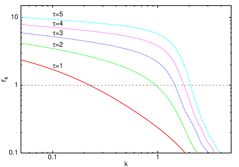
As we can see in Fig. 13, the evolution is driven towards large $r_{k}\gg 1$. Thus, in that limit,

$$(\theta_{k}+\phi_{k})^{\prime}=-{w^{\prime}\over w}\,{\sin 2\phi_{k}\over\sinh 2r_{k}}\to 0\,,$$

and therefore $\theta_{k}+\phi_{k}\to$ const. We can always choose this constant to be zero, so that the real and imaginary components of the field and momentum modes become

$$f_{k1}={1\over\sqrt{2k}}\,e^{r_{k}}\,\cos\phi_{k}\,,\hskip 45.52458ptf_{k2}={1\over\sqrt{2k}}\,e^{-r_{k}}\,\sin\phi_{k}\,,$$ (114)

$$g_{k1}=\sqrt{k\over 2}\,e^{-r_{k}}\,\cos\phi_{k}\,,\hskip 56.9055ptg_{k2}=\sqrt{k\over 2}\,e^{r_{k}}\,\sin\phi_{k}\,.$$ (115)

It is clear that, in the limit of large squeezing $(r_{k}\to\infty)$, the field mode $f_{k}$ becomes purely real, while the momentum mode $g_{k}$ becomes pure imaginary. This means that the field and momentum operators (20) become, in that limit,

$$\left.\begin{array}[]{l}\hat{y}({\bf k},\tau)\ \to\ \sqrt{2k}\,f_{k1}(\tau)\,\hat{y}({\bf k},\tau_{0})\\[5.69054pt] \hat{p}({\bf k},\tau)\ \to\ \sqrt{2k}\,g_{k2}(\tau)\,\hat{y}({\bf k},\tau_{0})\end{array}\right\}\ \Rightarrow\hskip 28.45274pt\hat{p}({\bf k},\tau)\ \to\ {g_{k2}(\tau)\over f_{k1}(\tau)}\,\hat{y}({\bf k},\tau)\,.$$ (116)

As a consequence of this squeezing, information about the initial momentum $\hat{p}_{0}$ distribution is lost, and the positions (or field amplitudes) at different times commute,

$$\Big{[}\hat{y}({\bf k},\tau_{1}),\ \hat{y}({\bf k},\tau_{2})\Big{]}\to{1\over 2}e^{-2r_{k}}\,\cos^{2}\phi_{k}\approx 0\,.$$ (117)

The last result defines what is known as a quantum non-demolition (QND) variable, which means that one can perform successive measurements of this variable with arbitrary precision without modifying the wave function. Note that $y=\delta\phi$ is the amplitude of fluctuations of the Higgs field after inflation, so what we have found is: first, that the amplitude is distributed as a classical gaussian random field with probability (31); and second that we can measure its amplitude at any time, and as much as we like, without modifying the distribution function.

In a sense, this problem is similar to that of a free non-relativistic quantum particle, described initially by a minimum wave packet, with initial expectation values $\langle x\rangle_{0}=x_{0}$ and $\langle p\rangle_{0}=p_{0}$, which becomes broader by its unitary evolution, and at late times $(t\gg mx_{0}/p_{0})$ this gaussian state becomes an exact WKB state, $\Psi(x)=\Omega_{R}^{-1/2}\,\exp(-\Omega\,x^{2}/2)$, with ${\rm Im}\,\Omega\gg{\rm Re}\,\Omega$ (i.e. high squeezing limit). In that limit, $[\hat{x},\ \hat{p}]\approx 0$, and we have lost information about the initial position $x_{0}$ (instead of the initial momentum like in our case), $\hat{x}(t)\to\hat{p}(t)\,t/m=p_{0}t/m$ and $\hat{p}(t)=p_{0}$. Therefore, not only $[\hat{p}(t_{1}),\ \hat{p}(t_{2})]=0$, but also, at late times, $[\hat{x}(t_{1}),\ \hat{x}(t_{2})]\approx 0$.

Appendix B The Wigner function

The Wigner function is the best candidate for a probability density of a quantum mechanical system in phase-space Wigner . Of course, we know from Quantum Mechanics that such a probability distribution function cannot exist, but the Wigner function is just a good approximation to that distribution. Furthermore, in the case of a gaussian state, this function is positive definite, and can in fact play the role of a classical probability distribution for the quantum state.

Consider a quantum state described by a density matrix $\rho$. Then the Wigner function can be written as

$$W(y_{k}^{0},{y_{k}^{0}}^{*},p_{k}^{0},{p_{k}^{0}}^{*})=\int\int\,{dx_{1}\,dx_{2}\over(2\pi)^{2}}\,e^{-i(p_{1}\,x_{1}+p_{2}\,x_{2})}\,\left\langle y-{x\over 2},\tau\right|\rho\left|y+{x\over 2},\tau\right\rangle\,.$$ (118)

If we substitute for the state our vacuum initial condition $\rho=|\Psi_{0}\rangle\langle\Psi_{0}|$, with $\Psi_{0}$ given by the gaussian wave function (30), we can perform the integration explicitly to obtain

$$W_{0}(y_{k}^{0},{y_{k}^{0}}^{*},p_{k}^{0},{p_{k}^{0}}^{*})={1\over\pi^{2}}\,\exp\left(-{|y|^{2}\over|f_{k}|^{2}}-4|f_{k}|^{2}\Big{|}p-{F_{k}\over|f_{k}|^{2}}\,y\Big{|}^{2}\right)\equiv\Phi(y_{1},\,p_{1})\,\Phi(y_{2},\,p_{2})\hskip 5.69054pt$$

$$\Phi(y_{1},\,p_{1})={1\over\pi}\,\exp\left\{-\Big{(}{y_{1}^{2}\over|f_{k}|^{2}}+4|f_{k}|^{2}\,\bar{p}_{1}^{2}\Big{)}\right\}\,,\hskip 28.45274pt\bar{p}_{1}\equiv p_{1}-{F_{k}\over|f_{k}|^{2}}\,y_{1}\,.\hskip 28.45274pt$$ (119)

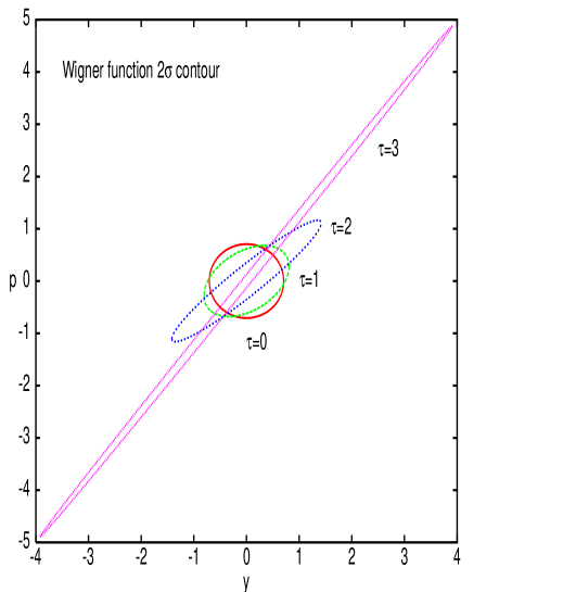
However, at time $\tau=\tau_{0}$, we have $y_{1}^{0}={1\over\sqrt{2k}}=|f_{k}(\tau_{0})|\,,\ p_{1}^{0}=\sqrt{k\over 2}=(2|f_{k}(\tau_{0})|)^{-1}$, and $F_{k}(\tau_{0})=0$, so that $\bar{p}_{1}^{0}=p_{1}^{0}$, and therefore $W_{0}$ describes a symmetric gaussian in phase space, with the same dispersion in both $y$ and $p$-directions. The $2\sigma$ contours of this distribution satisfy

$${y_{1}^{2}\over|f_{k}|^{2}}+4|f_{k}|^{2}\,\bar{p}_{1}^{2}\ \leq\ 1\hskip 14.22636pt\longrightarrow\hskip 14.22636pt{y_{1}^{2}\over{y_{1}^{0}}^{2}}+{p_{1}^{2}\over{p_{1}^{0}}^{2}}\leq 1\,,\hskip 14.22636pt{\rm for}\ \tau=\tau_{0}\,,$$ (120)

which is a circle in phase space. On the other hand, for time $\tau\gg\tau_{0}$, we have

$$|f_{k}| \to {1\over\sqrt{2k}}\,e^{r_{k}}\sim y_{k}^{0}\,e^{r_{k}}\,,\hskip 42.67912pt{\rm growing\ mode}\,,\hskip 28.45274pt$$ (121)

$${1\over 2|f_{k}|} \to \sqrt{k\over 2}\,e^{-r_{k}}\sim p_{k}^{0}\,e^{-r_{k}}\,,\hskip 28.45274pt{\rm decaying\ mode}\,,\hskip 28.45274pt$$ (122)

so that the ellipse (120) becomes highly “squeezed”, see Fig. 14. Note that Liouville’s theorem implies that the volume of phase space is conserved under Hamiltonian (unitary) evolution, so that the area within the ellipse should be conserved, and as a consequence there is no entropy production in this process. As the probability distribution compresses (squeezes) along the $p$-direction, it expands along the $y$-direction. At late times, the Wigner function is highly concentrated around the region

$$\bar{p}^{2}=\Big{(}p-{F_{k}\over|f_{k}|^{2}}\,y\Big{)}^{2}<{1\over 4|f_{k}|^{2}}\sim p_{0}^{2}\,e^{-2r_{k}}\ll 1\,.$$ (123)

We can thus take the above squeezing limit in the Wigner function (B) and write the exponential term as a Dirac delta function,

$$W_{0}(y,p)\stackrel{{\scriptstyle r_{k}\to\infty}}{{\longrightarrow}}{1\over\pi^{2}}\,\exp\Big{\{}\!-{|y|^{2}\over|f_{k}|^{2}}\Big{\}}\ \delta\Big{(}p-{F_{k}\over|f_{k}|^{2}}\,y\Big{)}\,.$$ (124)

In this limit we have

$$\hat{p}_{k}(\tau)={F_{k}\over|f_{k}|^{2}}\,\hat{y}_{k}(\tau)\ \to\ {g_{k2}(\tau)\over f_{k1}(\tau)}\,\hat{y}_{k}(\tau)\,,$$ (125)

so we recover the previous result (116). This explains why we can treat the system as a classical gaussian random field: the amplitude of the field $y$ is uncertain with probability distribution (31), but once a measurement of $y$ is performed, we can automatically assign to it a definite value of the momentum, according to (116).

Figure 14: The 2$\sigma$ contour of the Wigner function (B) for the mode $k=1$, at times $\tau=0,1,2,3$. It is clear that, as time progresses, the ellipse (120) becomes more elongated (squeezed), without changing its area, while the main axis rotates counter-clockwise.

Note that the condition $F_{k}^{2}\gg 1$ is actually a condition between operators and their commutators/anticommutators. The Heisenberg uncertainty principle states that

$$\Delta_{\Psi}A\,\Delta_{\Psi}B\geq{1\over 2}\,\Big{|}\langle\Psi|[A,\ B]|\Psi\rangle\Big{|}\,,$$

for any two hermitian operators (observables) in the Hilbert space of the wave function $\Psi$. In our case, and in Fourier space, this corresponds to

$$\Delta_{\Psi}y^{2}(k)\,\Delta_{\Psi}p^{2}(k)=F_{k}^{2}(\tau)+{1\over 4}\geq{1\over 4}\,\Big{|}\langle\Psi|[y_{k}(\tau),\ p^{\dagger}_{k}(\tau)]|\Psi\rangle\Big{|}^{2}\,,$$ (126)

with $|\Psi\rangle=|0,\tau_{0}\rangle$ the vacuum wave function. On the other hand, $F_{k}$ can be written as

$$F_{k}={1\over 2}\,\langle\Psi|\hat{p}({\bf k},\tau)\,\hat{y}^{\dagger}({\bf k},\tau)+\hat{y}({\bf k},\tau)\,\hat{p}^{\dagger}({\bf k},\tau)|\Psi\rangle=-\,{i\over 2}\,(g_{k}\,f_{k}^{*}-f_{k}\,g_{k}^{*})={\rm Im}\,(f_{k}^{*}\,g_{k})\,,$$ (127)

where we have used (20) and $\ a({\bf k},\tau_{0})|\Psi\rangle=0,\ \forall{\bf k}$. The above relation just indicates that, for any state $\Psi$, the condition of classicality $(F_{k}\gg 1)$ is satisfied whenever, for that state,

$$\langle\{\hat{y}_{k}(\tau),\ \hat{p}_{k}^{\dagger}(\tau)\}\rangle\gg\langle|[\hat{y}_{k}(\tau),\ \hat{p}_{k}^{\dagger}(\tau)]|\rangle=\hbar\equiv 1\,.$$ (128)

It is this condition which allows one to substitute quantum averages of arbitrary functions $G$ of the position and momentum operators by classical ensemble averages of the same function $G$, weighted with the Wigner probability distribution function, or schematically,

$$\langle\Psi|G(\hat{y}_{k},\ \hat{p}_{k})|\Psi\rangle = \int dy_{k}\,dp_{k}\,G(y_{k},\,p_{k})\,W_{0}(y_{k},\,p_{k})+{\cal O}(\hbar)$$ (129)

$$\stackrel{{\scriptstyle r_{k}\to\infty}}{{\longrightarrow}} {1\over\pi^{2}}\int dy_{k}\,G\Big{(}y_{k},\,{F_{k}(\tau)\over|f_{k}|^{2}}\,y_{k}\Big{)}\,e^{\displaystyle-{y_{k}^{2}\over|f_{k}(\tau)|^{2}}}\,,$$ (130)

where we have used Eq. (124). As long as $F_{k}(\tau)\gg 1$, we can describe the evolution of our quantum system as that of a classical gaussian random field. Note that, in this limit, we can ignore the normal ordering of the operators in $G(\hat{y}_{k},\,\hat{p}_{k})$.

Appendix C Non-linear evolution in perturbation theory

In this appendix we will give details of how to perform perturbative calculations of the non-linear evolution of our quantum system. We will also illustrate the perturbative expansion of the correlation functions of a classical random field. To simplify the expressions we will consider the case of a single component real scalar(Higgs) field, but generalisation to complex or multiple component case is straightforward.

Our goal is to compute the expectation values of products of fields at different points:

$$\langle\phi(\tau_{1},{\bf x}_{1})\ldots\phi(\tau_{n},{\bf x}_{n})\rangle$$ (131)

(In this section we will use the symbol $\phi$ instead of $y$ for the Higgs field). Here $\phi(\tau,{\bf x})$ denotes the Heisenberg picture field operator, whose relation to the Schrödinger picture one $\phi_{s}({\bf x})$ is as follows:

$$\phi(\tau,{\bf x})={\cal U}^{\dagger}(\tau)\,\phi_{s}({\bf x})\,{\cal U}(\tau)$$ (132)

where ${\cal U}(\tau)$ is the evolution operator, satisfying:

$${\cal U}^{\prime}(\tau)=-i{\mathbf{H}}\,{\cal U}(\tau)$$ (133)

where the prime stands for derivative with respect to $\tau$ and ${\mathbf{H}}$ is the full Hamiltonian. Notice that since the Hamiltonian depends explicitly on time, the evolution operator cannot be written as $\exp\{-i\tau{\mathbf{H}}\}$. If we set $\lambda$ to zero we get the quadratic Hamiltonian ${\mathbf{H}}_{0}$ considered in the gaussian approximation. The corresponding evolution operator is ${\cal U}_{0}(\tau)$. Now we go over to the interaction representation by writing:

$${\cal U}(\tau)={\cal U}_{0}(\tau)\,{\mathbf{\Omega}}(\tau)$$ (134)

where ${\mathbf{\Omega}}(\tau)$ is the characteristic Moller type operator which satisfies the equation:

$${\mathbf{\Omega}}^{\prime}(\tau)=-i\,{\cal U}_{0}^{\dagger}(\tau)\,{\mathbf{H}}_{\mbox{\small int}}\,{\cal U}_{0}(\tau)\,{\mathbf{\Omega}}=-i\,{\mathbf{H}}_{\mbox{\small int}}^{(0)}(\tau)\,{\mathbf{\Omega}}$$ (135)

where ${\mathbf{H}}_{\mbox{\small int}}^{(0)}(\tau)$ is the interaction hamiltonian in the interaction representation. The equation for ${\mathbf{\Omega}}$ can be solved in terms of the time-ordered exponential:

$${\mathbf{\Omega}}(\tau)=T\exp\{-i\!\int_{0}^{\tau}\!dt\,{\mathbf{H}}_{\mbox{\small int}}^{(0)}(t)\}$$ (136)

This can be used to express the Heisenberg representation fields in terms of the (gaussian) interaction representation fields:

$$\phi(\tau,{\bf x})=T^{\prime}\exp\{i\!\int_{0}^{\tau}\!dt\,{\mathbf{H}}_{\mbox{\small int}}^{(0)}(t)\}\;\phi_{0}(\tau,{\bf x})\ T\exp\{-i\!\int_{0}^{\tau}\!dt\,{\mathbf{H}}_{\mbox{\small int}}^{(0)}(t)\}$$ (137)

In the $T$-exponential time grows from right to left and in the $T^{\prime}$-exponential left to right. To obtain the perturbative expansion one has to expand the $T$-exponential and ${\mathbf{H}}_{\mbox{\small int}}^{(0)}$ in powers of $\lambda$. The latter has the form

$${\mathbf{H}}_{\mbox{\small int}}^{(0)}(\tau)=\lambda\int\!d^{3}x\,\left(\frac{1}{4}\phi_{0}^{4}(\tau,{\bf x})-\frac{3(\delta_{1}+\delta_{2}\tau)}{2}\phi_{0}^{2}(\tau,{\bf x})\right)+O(\lambda^{2})$$ (138)

where the second piece is the counter-term needed to renormalise to this order. Then, substituting the expression of the field inside the expectation values, everything reduces to expectation values of products of interaction representation fields $\phi_{0}(\tau,{\bf x})$. The latter reduce, by Wick’s theorem, to products of two-point functions:

$$G^{(0)}(\tau,\tau^{\prime},{\bf x}-{\bf x}^{\prime})\equiv\langle\phi_{0}(\tau,{\bf x})\phi_{0}(\tau^{\prime},{\bf x}^{\prime})\rangle=\int\frac{d^{3}k}{(2\pi)^{3}}e^{i{\bf k}({\bf x}-{\bf x}^{\prime})}\,f_{k}(\tau)f^{*}_{k}(\tau^{\prime})\,.$$ (139)

This can be decomposed into a real and imaginary part. The real part corresponds to the expectation value of the symmetrised product, which in the gaussian theory was chosen to match with the correlation function of the classical random field. The imaginary part is proportional to the commutator of the fields, which is a c-number.

We can illustrate the procedure by computing the 2-point function

$$\langle\phi(\tau,{\bf x})\phi(\tau^{\prime},{\bf x}^{\prime})\rangle=\int\frac{d^{3}k}{(2\pi)^{3}}e^{i{\bf k}({\bf x}-{\bf x}^{\prime})}\,\hat{G}(k,\tau,\tau^{\prime})$$ (140)

to order $\lambda$. Substituting the expression of the Heisenberg field for the $\tau>\tau^{\prime}$ case we get

$$\langle T^{\prime}\exp\{i\!\int_{0}^{\tau}dt\,{\mathbf{H}}_{\mbox{\small int}}^{(0)}(t)\}\,\phi_{0}({\bf x},\tau)\ T\exp\{-i\!\int_{\tau^{\prime}}^{\tau}dt\,{\mathbf{H}}_{\mbox{\small int}}^{(0)}(t)\}\,\phi_{0}({\bf x}^{\prime},\tau^{\prime})\,T\exp\{-i\!\int_{0}^{\tau^{\prime}}dt\,{\mathbf{H}}_{\mbox{\small int}}^{(0)}(t)\}\rangle$$

In case $\tau^{\prime}>\tau$ the factor sitting between the two fields has to be replaced by:

$$T^{\prime}\exp\{i\!\int_{\tau}^{\tau^{\prime}}dt\,{\mathbf{H}}_{\mbox{\small int}}^{(0)}(t)\}$$ (141)

Notice the peculiar time-ordering of the operators which differs from the customary perturbative evaluation of (Feynman) Green functions, which are time-ordered products of field operators.

To do the calculation to order $\lambda$ it is better to start by expressing the Heisenberg field to this order:

$$\phi(\tau,{\bf x}) = \phi_{0}(\tau,{\bf x})+i\int ds\,[{\mathbf{H}}_{\mbox{\small int}}^{(0)}(s),\phi_{0}(\tau,{\bf x})]+\ldots$$ (142)

$$= \phi_{0}(\tau,{\bf x})+i\lambda\int\!ds\,d^{3}z\;[\phi_{0}(s,{\bf z}),\phi_{0}(\tau,{\bf x})]\left(\phi_{0}^{3}(s,{\bf z})-3(\delta_{1}+\delta_{2}s)\phi_{0}(s,{\bf z})\right)\hskip 14.22636pt$$

Finally one obtains

$$\hat{G}(k,\tau,\tau^{\prime})=f_{k}(\tau)f^{*}_{k}(\tau^{\prime})+6\lambda\int_{0}^{\tau}ds\,A_{\mbox{\tiny ren}}(s)\,{\rm Im}\,[f_{k}(\tau)f_{k}^{*}(s)]\ f_{k}(s)f_{k}^{*}(\tau^{\prime})$$

$$+6\lambda\int_{0}^{\tau^{\prime}}ds\,A_{\mbox{\tiny ren}}(s)\,{\rm Im}\,[f_{k}(\tau^{\prime})f_{k}^{*}(s)]\ f_{k}(\tau)f_{k}^{*}(s)\,.$$ (143)

The meaning of $A_{\mbox{\tiny ren}}(\tau)$ is given in the main text, where one can also find the symmetrised Green function. Repeating the calculation for a Higgs field with $N_{c}$ real components one gets the same expression for each component replacing $6$ by $2(N_{c}+2)$.

We can compare with the classical evolution. We will use the same symbol for the classical field $\phi(\tau,{\bf x})$. The equations of motion

$$\phi^{\prime\prime}(\tau,{\bf x})=\Delta\phi(\tau,{\bf x})+\tau\phi(\tau,{\bf x})-\lambda\phi^{3}(\tau,{\bf x})$$ (144)

can be solved in perturbation theory in $\lambda$. The expansion is given in terms of tree graphs with lines associated to the retarded propagator:

$$G_{\mbox{\tiny ret}}(\tau,\tau^{\prime},{\bf x}-{\bf x}^{\prime})=-2\theta(\tau-\tau^{\prime})\,\int\frac{d^{3}k}{(2\pi)^{3}}e^{i{\bf k}({\bf x}-{\bf x}^{\prime})}\,{\rm Im}\,[f_{k}(\tau)f^{*}_{k}(\tau^{\prime})]\,.$$ (145)

If we now take $\phi(\tau=0,{\bf x})$, and $\pi(\tau=0,{\bf x})$, to be gaussian random fields, then the field at any other time becomes a non-gaussian random field. The correlation functions of this field can be computed in perturbation theory by combining the aforementioned expansion involving the retarded propagator and the expectation value of gaussian random field. To match with the quantum calculation at zero-order in $\lambda$, this has to be taken as the symmetrised version of Eq. 139 (this is just given by the Fourier transform of the symmetric part of $\Sigma$):

$$G^{(0)}_{\mbox{\tiny gauss}}(\tau,\tau^{\prime},{\bf x}-{\bf x}^{\prime})=\int\frac{d^{3}k}{(2\pi)^{3}}e^{i{\bf k}({\bf x}-{\bf x}^{\prime})}\,{\rm Re}\,[f_{k}(\tau)f_{k}^{*}(\tau^{\prime})]\,.$$ (146)

Notice that terms in the expansion can be associated with Feynman-type graphs, with modified rules involving two propagators ($G^{(0)}_{\mbox{\tiny gauss}}$ and $G_{\mbox{\tiny ret}}$). These, up to factors (including Heaviside $\theta$) coincide with the real and imaginary parts of the quantum propagator. Indeed, the calculation of the two-point correlation function to order $\lambda$ matches exactly with the symmetrised quantum two-point function to this order. For that one has to apply exactly the same renormalization to the classical and quantum theories.

Differences can arise to higher order. Essentially, the retarded-imaginary propagator in the classical theory cannot form loops by itself. since it arose from the expansion of the field equations. This need not be the case in the quantum theory. For example to second order in $\lambda$ there is a contribution to the two-point function given by the sunset diagram, with three imaginary propagators joining the two vertices. However, for low-momenta flowing through the lines (and large enough times) the dramatic difference in size of the real and imaginary parts of $f_{k}(\tau)f^{*}_{k}(\tau^{\prime})$ justifies that the classical approximation would still be reasonably good. A more thorough investigation of these matters is interesting but exceeds the realm of this paper.

References

- (1) D.A. Kirzhnits, JETP Lett. 15 (1972) 529; D.A. Kirzhnits and A.D. Linde, Phys. Lett. 42B (1972) 471; Sov. Phys. JETP 40 (1974) 628; Ann. Phys. 101 (1976) 195; S. Weinberg, Phys. Rev. D9 (1974) 3320; L. Dolan and R. Jackiw, Phys. Rev. D9 (1974) 3357; D. A. Kirzhnits & A. D. Linde, Ann. Phys. 101 (1976) 195.
- (2) T. W. Kibble, J. Phys. A 9 (1976) 1387; M. B. Hindmarsh and T. W. Kibble, Rept. Prog. Phys. 58 (1995) 477 [hep-ph/9411342]; W. H. Zurek, Nature 317 (1985) 505; Phys. Rept. 276 (1996) 177 [cond-mat/9607135].
- (3) F. Cooper, S. Habib, Y. Kluger and E. Mottola, “Nonequilibrium dynamics of symmetry breaking in lambda Phi**4 field theory,” Phys. Rev. D 55 (1997) 6471 [hep-ph/9610345]; F. Cooper, S. Habib, Y. Kluger, E. Mottola, J. P. Paz and P. R. Anderson, “Nonequilibrium quantum fields in the large N expansion,” Phys. Rev. D 50 (1994) 2848 [hep-ph/9405352].
- (4) D. Boyanovsky and H. J. de Vega, “Dynamics of symmetry breaking out of equilibrium: From condensed matter to QCD and the early universe,” hep-ph/9909372; “Dynamics of symmetry breaking in FRW cosmologies: Emergence of scaling,” Phys. Rev. D 61 (2000) 105014 [hep-ph/9911521]; D. Boyanovsky, D. Cormier, H. J. de Vega, R. Holman, A. Singh and M. Srednicki, “Scalar field dynamics in Friedman Robertson Walker spacetimes,” Phys. Rev. D 56 (1997) 1939 [hep-ph/9703327]; D. Boyanovsky, H. J. de Vega, R. Holman and J. Salgado, “Non-equilibrium Bose-Einstein condensates, dynamical scaling and symmetric evolution in large N phi**4 theory,” Phys. Rev. D 59 (1999) 125009 [hep-ph/9811273].
- (5) J. Baacke, K. Heitmann and C. Patzold, “Nonequilibrium dynamics: A renormalized computation scheme,” Phys. Rev. D 55 (1997) 2320 [hep-th/9608006]; “Nonequilibrium dynamics: Preheating in the SU(2) Higgs model,” Phys. Rev. D 55 (1997) 7815 [hep-ph/9612264]; “Renormalization of nonequilibrium dynamics in FRW cosmology,” Phys. Rev. D 56 (1997) 6556 [hep-ph/9706274]; J. Baacke and S. Michalski, “Nonequilibrium evolution in scalar O(N) models with spontaneous symmetry breaking,” Phys. Rev. D 65 (2002) 065019 [hep-ph/0109137].
- (6) G. Aarts and J. Berges, “Classical aspects of quantum fields far from equilibrium,” Phys. Rev. Lett. 88 (2002) 041603 [hep-ph/0107129].
- (7) J. Smit, J. C. Vink and M. Salle, “Initial conditions for simulated ’tachyonic preheating’ and the Hartree ensemble approximation”, hep-ph/0112057; “New initial conditions for quantum field simulations after a quench,” Nucl. Phys. Proc. Suppl. 106 (2002) 540 [hep-lat/0110093].
- (8) A.D. Linde, Phys. Lett. B259 (1991) 38; “Hybrid inflation,” Phys. Rev. D 49 (1994) 748 [astro-ph/9307002].
- (9) J. García-Bellido and A. D. Linde, “Preheating in hybrid inflation,” Phys. Rev. D 57 (1998) 6075 [hep-ph/9711360].
- (10) L. Kofman, A. Linde and A. A. Starobinsky, “Reheating after inflation,” Phys. Rev. Lett. 73 (1994) 3195 [hep-th/9405187]; “Towards the theory of reheating after inflation,” Phys. Rev. D 56 (1997) 3258 [hep-ph/9704452]; P. B. Greene, L. Kofman, A. Linde and A. A. Starobinsky, Phys. Rev. D 56 (1997) 6175 [hep-ph/9705347].
- (11) S. Yu. Khlebnikov and I. I. Tkachev, ‘Classical decay of the inflaton,” Phys. Rev. Lett. 77 (1996) 219 [hep-ph/9603378]; “Resonant decay of Bose condensates,” Phys. Rev. Lett. 79 (1997) 1607 [hep-ph/9610477];
- (12) T. Prokopec and T. G. Roos, “Lattice study of classical inflaton decay,” Phys. Rev. D 55 (1997) 3768 [hep-ph/9610400].
- (13) G. Felder and L. Kofman, “The development of equilibrium after preheating,” Phys. Rev. D 63 (2001) 103503 [hep-ph/0011160].
- (14) G. N. Felder, J. García-Bellido, P. B. Greene, L. Kofman, A. D. Linde and I. Tkachev, “Dynamics of symmetry breaking and tachyonic preheating,” Phys. Rev. Lett. 87 (2001) 011601 [hep-ph/0012142]; G. N. Felder, L. Kofman and A. D. Linde, “Tachyonic instability and dynamics of spontaneous symmetry breaking,” Phys. Rev. D 64 (2001) 123517 [hep-th/0106179].
- (15) J. García-Bellido and E. Ruiz Morales, “Particle production from symmetry breaking after inflation and leptogenesis,” Phys. Lett. B 536 (2002) 193 [hep-ph/0109230].
- (16) E. J. Copeland, S. Pascoli and A. Rajantie, “Dynamics of tachyonic preheating after hybrid inflation,” Phys. Rev. D 65 (2002) 103517 [hep-ph/0202031].
- (17) A. H. Guth and S. Y. Pi, “The Quantum Mechanics Of The Scalar Field In The New Inflationary Universe,” Phys. Rev. D 32 (1985) 1899.
- (18) D. Polarski and A. A. Starobinsky, “Semiclassicality and decoherence of cosmological perturbations,” Class. Quant. Grav. 13 (1996) 377 [gr-qc/9504030].
- (19) C. Kiefer, D. Polarski and A. A. Starobinsky, “Quantum-to-classical transition for fluctuations in the early universe,” Int. J. Mod. Phys. D 7 (1998) 455 [gr-qc/9802003].
- (20) J. Lesgourgues, D. Polarski and A. A. Starobinsky, “Quantum-to-classical transition of cosmological perturbations for non-vacuum initial states,” Nucl. Phys. B 497 (1997) 479 [gr-qc/9611019]; J. Lesgourgues, Ph.D. Thesis (1998).
- (21) J. García-Bellido, D. Y. Grigoriev, A. Kusenko and M. E. Shaposhnikov, “Non-equilibrium electroweak baryogenesis from preheating after inflation,” Phys. Rev. D 60 (1999) 123504 [hep-ph/9902449]
- (22) L. M. Krauss and M. Trodden, “Baryogenesis below the electroweak scale,” Phys. Rev. Lett. 83 (1999) 1502 [hep-ph/9902420].
- (23) A. Rajantie, P. M. Saffin and E. J. Copeland, “Electroweak preheating on a lattice,” Phys. Rev. D 63 (2001) 123512 [hep-ph/0012097]; E. J. Copeland, D. Lyth, A. Rajantie and M. Trodden, “Hybrid inflation and baryogenesis at the TeV scale,” Phys. Rev. D 64 (2001) 043506 [hep-ph/0103231].
- (24) J.M. Bardeen, J.R. Bond, N. Kaiser and A.S. Szalay, Astrophys. J. 304 (1986) 15.
- (25) G. R. Dvali, Q. Shafi and R. Schaefer, “Large Scale Structure And Supersymmetric Inflation Without Fine Tuning,” Phys. Rev. Lett. 73 (1994) 1886 [hep-ph/9406319].
- (26) M. Bastero-Gil, S. F. King and J. Sanderson, “Preheating in supersymmetric hybrid inflation,” Phys. Rev. D 60 (1999) 103517 [hep-ph/9904315].
- (27) G. N. Felder, J. García-Bellido, P. B. Greene, L. Kofman and A. D. Linde, “Tachyonic Preheating in Hybrid Inflation,” in preparation.
- (28) J. García-Bellido, A. D. Linde and D. Wands, “Density perturbations and black hole formation in hybrid inflation,” Phys. Rev. D 54 (1996) 6040 [astro-ph/9605094].
- (29) D. H. Lyth and E. D. Stewart, “Thermal inflation and the moduli problem,” Phys. Rev. D 53 (1996) 1784 [hep-ph/9510204].
- (30) D. H. Lyth and A. Riotto, “Particle physics models of inflation and the cosmological density perturbation,” Phys. Rept. 314 (1999) 1 [hep-ph/9807278].
- (31) M. Abramowitz and I.A. Stegun, Handbook of Mathematical Functions, Dover, New York, 1970.
- (32) M. J. Bowick and A. Momen, “Domain formation in finite-time quenches,” Phys. Rev. D 58 (1998) 085014 [hep-ph/9803284].
- (33) T. Asaka, W. Buchmuller and L. Covi, “False vacuum decay after inflation,” Phys. Lett. B 510 (2001) 271 [hep-ph/0104037].
-
(34)
J. García-Bellido, “Particle Production and
Symmetry Breaking after Hybrid Inflation”, Plenary talk at
COSMO-01, International Workshop on PARTICLE PHYSICS AND THE EARLY
UNIVERSE, August 30 - September 4, 2001, Rovaniemi, Finland. For a
transcript
of the talk see http://www.physics.helsinki.fi/cosmo_01/friday/Garcia-Bellido.pdf - (35) G. Aarts and J. Smit, “Finiteness of hot classical scalar field theory and the plasmon damping rate,” Phys. Lett. B 393 (1997) 395 [hep-ph/9610415]. G. Aarts and J. Smit, “Classical approximation for time-dependent quantum field theory: Diagrammatic analysis for hot scalar fields,” Nucl. Phys. B 511 (1998) 451 [hep-ph/9707342]
- (36) D. Y. Grigoriev and V. A. Rubakov, “Soliton Pair Creation At Finite Temperatures. Numerical Study In (1+1)-Dimensions,” Nucl. Phys. B 299 (1988) 67; D. Y. Grigoriev, V. A. Rubakov and M. E. Shaposhnikov, “Topological Transitions At Finite Temperatures: A Real Time Numerical Approach,” Nucl. Phys. B 326 (1989) 737; K. Kajantie, M. Laine, K. Rummukainen and M. E. Shaposhnikov, “Generic rules for high temperature dimensional reduction and their application to the standard model,” Nucl. Phys. B 458 (1996) 90 [hep-ph/9508379].
- (37) A.J.S. Hamilton, J.R. Gott III, D. Weinberg, Astrophys. J. 309 (1986) 1.
- (38) G. Felder and I.I Tkachev, “LATTICEEASY: A program for lattice simulations of scalar fields in an expanding Universe”, hep-ph/0011159.
- (39) E. P. Wigner, “On the quantum correction for thermodynamic equlibrium,” Phys. Rev. 40 (1932) 749.