Some Recent Developments in Perturbative Quantum Chromodynamics

Abstract

This talk reviews some recent trends in perturbative quantum chromodynamics, with emphasis on higher orders in perturbation theory, resummation and power corrections.

1 INTRODUCTION

This talk begins with a few general comments about the place of QCD studies. I go on to give a few words on the central role played by factorization and related concepts. A brief mention of some important steps forward in multiloop calculations is followed by a description of progress in abstracting classes of corrections at arbitrary order in perturbation theory. I will argue that the interplay of resummation with power corrections is a link between perturbation theory and the nonperturbative degrees of freedom of QCD.

A preliminary message in this talk is that QCD should be thought of as the exemplary field theory, one which illustrates all of the paradigms of what might be called “postmodern” particle physics, characterized by pairs of complementary concepts, as illustrated in Fig. 1.

       

Figure 1: Dual concepts.

QCD is the meeting ground of all the interactions of the standard model, and indeed, although it has only a single dimensional scale itself, $\Lambda_{\rm QCD}$, the influence of electroweak scales, through the W, Z and quark masses, is profound. At the same time, QCD generates its own secondary scales, though chiral symmetry breaking, confinement and vacuum structure. In so doing, it provides a tapestry of effective theories, each fitting into an energy range appropriate to a particular set of states. Among this list are perturbative QCD, heavy quark effective theory, non-relativistic QCD, lattice QCD, and nuclear physics. There is no doubt that QCD is “correct”, at least the way classical electricity and magnetism is correct, as itself an effective theory appropriate to a wide range of phenomena. Tests of QCD are, in this sense, tests of quantum field theory itself.

Figure 2: $F_{2}$ data

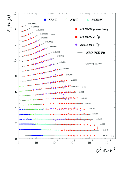
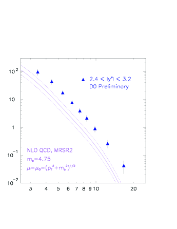
We are in a “golden age” for hadronic data, both in coverage and quality. The great accelerators of the nineteen nineties, HERA, the Tevatron, SLC and LEP, brought about a veritable revolution in strong interaction data. Our standards for judging success in fits to this data have correspondingly tightened. In this light, we can judge the experimental and theoretical successes and limitations of our description of deep-inelastic structure functions, Fig. 2, side-by-side with data on the transverse momentum distribution of b quarks, Fig. 3.

Figure 3: b quark data

2 UNITY OF QCD FACTORIZATIONS

The basis of perturbative QCD (PQCD) is in asymptotic freedom, applied to quantities that are infrared safe, that is, which depend only upon one (or more) momentum scales much larger than $\Lambda_{\rm QCD}$, up to corrections that can be estimated. For the simplest cases, observables like $\rm e^{+}e^{-}$ total and jet cross sections, it is convenient to choose the (renormalization) scale of the QCD coupling to equal the hard scale, $Q$,

$$Q^{2}\;\hat{\sigma}(Q^{2},\mu^{2},\alpha_{s}(\mu))$$ (1)

$$=\sum_{n}c_{n}(Q^{2}/\mu^{2})\;\alpha_{s}^{n}(\mu)+{\cal O}\left({1\over Q^{p}}\right)$$

$$=\sum_{n}c_{n}(1)\;\alpha_{s}^{n}(Q)+{\cal O}\left({1\over Q^{p}}\right)\,.$$

In the second form, the cross section is an expansion in a small parameter $\alpha_{s}(Q)$, with dimensionless coefficients. Corrections are suppressed by powers of the large scale. There are two challenges in treating infrared safe cross sections: the calculation of the $c_{n}$, and the interpretation and estimation of power corrections.

The set of infrared safe observables is rather limited. The applicability of perturbative methods is greatly expanded by factorization, which can be applied whenever an observable can be written as a product, or a convolution (denoted $\otimes$), of a short-distance function, times one or more functions that absorb nonperturbative, long-distance dynamics,

$$Q^{2}\sigma(Q,m) = \omega_{\rm SD}(Q/\mu,\alpha_{s}(\mu))\otimes f_{\rm LD}(\mu,m)$$ (2)

$$+{\cal O}\left({1\over Q^{p}}\right)\,,$$

where $\mu$ is the factorization scale, which separates the short- and long-distance components. This sort of factorization is familiar from deep-inelastic scattering (DIS) inclusive cross sections, where the $f$’s are parton distributions (PDFs), and from hard scattering cross sections at hadronic colliders, but it also applies, in varying forms, to amplitudes for exclusive processes, such as B decays and deeply-virtual Compton scattering, It also applies to jet cross sections in $\rm e^{+}e^{-}$ annihilation, for events where the jets are very narrow, and where the cross section is sensitive to relatively long-time behavior.

Different processes demand different proofs for their factorizations, but there are a number of common themes. At the basis of all factorization is the quantum-mechanical incoherence between short- with long-distance dynamics, and also between different sources of long-distance dynamics that develop at spacelike separations. The first allows the operator product expansion in DIS, the second justifies factorization for hadronic collisions.

The proverbial “new physics” is to be found in $\omega_{\rm SD}$; the long-distance $f_{\rm LD}$’s are “universal”, simply in the sense that they do not depend on what’s going on at short distances. Factorization may be regarded from complementary viewpoints. On the one hand, we may think of $\omega_{\rm SD}$ as the perturbation expansion in a theory with $f_{\rm LD}$ an IR regulator. This would be a “Wilsonian” point of view, with $\mu$ as an infrared cutoff. Another view is to describe $f_{\rm LD}$ as a matrix element in an effective theory with $\hat{\sigma}_{\rm SD}$ a matching coefficient, and $\mu$ the renormalization scale.

However we describe factorization, it can be useful only when the factorization scale $\mu$ is large enough that we can use perturbation theory to compute the short-distance function. A consequence of this rather simple observation is that, whenever there is factorization, there is a calculable evolution, which can be derived from the independence of the physical cross section from the factorization scale. Denoting infrared mass scales by $m$, we have

$$0=\mu{d\over d\mu}\ln\sigma_{\rm phys}(Q,m)$$ (3)

$$=\mu{d\over d\mu}\ln\left\{\omega_{\rm SD}(Q/\mu,\alpha_{s}(\mu))\otimes f_{\rm LD}(\mu,m)\right\}\,,$$

so that, very schematically,

$$\mu{d\ln f\over d\mu}=-P(\alpha_{s}(\mu))=-\mu{d\ln\omega\over d\mu}\,,$$ (4)

where the (splitting) function $P(\alpha_{s})$ can depend only on the variables held in common between $\omega_{\rm SD}$ and $f_{\rm LD}$, which are the coupling and an appropriate convolution variable (or moment variable). For factorizations like Eq. (2), where corrections are power-suppressed, all orders in $\alpha_{s}$ respect the form of the evolution equation. The solution to any evolution equation can be thought of as a resummation of the theory,

$$\ln\sigma_{\rm phys}(Q,m)\sim\exp\left\{-\int^{Q}{d\mu^{\prime}\over\mu^{\prime}}P\left(\alpha_{s}(\mu^{\prime})\right)\right\}\,.$$ (5)

Let’s first discuss examples of progress in the calculations of the short-distance functions, and then return to examples of what we have learned over the past few years from resummations.

3 HIGHER LOOPS & JETS

3.1 Toward a Two-loop Phenomenology

The perturbative running coupling is typically quoted at the scale of the Z mass, $\alpha_{s}(M_{Z})\sim 0.12$. In a rough sense, then, we can estimate that corrections at $\alpha_{s}^{2}$ are of order 1%. Now it so happens that one percent accuracy in jet cross sections at a linear collider would allow a much more accurate extrapolation of Standard Model scales through their logarithmic evolution to energies characteristic of grand unification. At the same time, one percent is roughly the level to which nonperturbative corrections have shrunk for inclusive jet cross sections at a few hundreds of GeV. The scales of the physics in which we are most interested strongly invite us to two loops.

Referring to Eq. (1), a summary of the status of $c_{n}$’s is, they are known at next-to-leading order (NLO) up to four jets $\rm e^{+}e^{-}$, and up to NNLO only for one-scale problems: the $\rm e^{+}e^{-}$ total cross section and DIS structure functions. Two loops is the frontier of finite-order PQCD. The splitting function for DIS factorization (the DGLAP kernels), $P(z)$ are themselves known at order $\alpha_{s}^{2}$, although to make full use of two-loop calculations of short-distance functions, we should know them at three loops. Here, progress has been made, and an increasing number of moments $\int dzz^{n}P(z)$, at $\alpha_{s}^{3}$ have been reported [1, 2]. Using these results, there is a budding phenomenology of DIS at NNLO [3].

In very recent and substantial progress, two-loop QCD corrections to $2\rightarrow 2$ quark and gluon scattering amplitudes have been computed [4, 5]. These results are the first step along what promises to be a very steep path to the computation of cross sections, including phase-space integrals at NNLO. In the estimates of the experts, we are still a number of years away from true NNLO jet cross sections, but it should be worth the wait.

3.2 Energy Flow

One fundamental use of the two-loop scattering amplitudes that are beginning to appear, and the corresponding $2\rightarrow 3$ and $2\rightarrow 4$ processes that will follow, is in the computation of jet production in hadronic collisions, which will be a background (and signal) for new physics. Closely related calculations will also be applied to event shapes in $\rm e^{+}e^{-}$ annihilation [6]. NLO inclusive jet cross sections are a familiar feature from the Tevatron.

For the most part, jet events are identified “algorithmically”, by a series of steps that assigns particles (or calorimeter towers) in an event to a list of jets. Jet algorithms have become quite sophisticated, and are becoming more so [7]. Newer versions avoid some of the technical problems that have been associated with previous implementations. The primary requirement of a jet algorithm is infrared safety, that is, it should specify cross sections that are factorizable into PDFs and a pertrubative short distance function.

Here, I would like to mention a class of observables that are supplements to jet algorithms, and which quantify the flow of energy [8, 9]. One of the first, and still familiar, infrared safe cross sections in electron-positron annihilation is the energy-energy correlation [10]. Energy flow variables are closely related to this concept. These observables are weighted sums that are linear in the momenta of final-state particles. In a notation based on the formalism of [8], they may be represented conveniently as

$$J_{\mu}(m\equiv\{\eta,\phi\})$$ (6)

$$=\int dm^{\prime}\,P_{\mu}(m^{\prime})\,\times{\cal W}(m^{\prime}-m)\,,$$

where the integral is over directions $m^{\prime}$ and ${\cal W}$ is the weighting function, and where

$$P_{\mu}(m^{\prime}) \equiv \sum_{i=1}^{N}\;p_{\mu}^{i}\,\delta\left(m^{\prime}-m_{i}\right)\,,$$ (7)

for a state with $N$ final state particles. Properly chosen, the weight function themselves can distinguish the gross features of jet events [8, 9]. They may also be readily treated with the techniques of resummation and, eventually, estimates of power corrections, about which we shall say a bit more below.

A feature of jet cross sections is that they discard much of event structure. It may be valuable to measure a variety of weighted energy flow correlations for events with large transverse momenta, to derive information that is complementary to differential jet cross sections in terms of transverse momentum and rapidity. For example, correlations involving relatively soft particles may well contain information on the flow of color at short distances.

In time, our understanding of QCD will progress, and we would like to be able to go back to the data to ask new questions. Certainly, an ideal to be sought after is to free the data from contemporary theory. This is a difficult task, and complete archival accessibility may be an unattainable goal. Nevertheless, it is worthwhile to try to keep the reported data as close as possible to the observables themselves, rather than to report on secondary quantities. Thus, in DIS, it is important to make available measured cross sections, in addition to structure functions, and certainly to fitted parton distributions.

4 THRESHOLD RESUMMATION

Now let us turn to an example that shows how it is sometimes possible to organize and compute a class of corrections to all orders in perturbation theory, in this case through threshold resummation [11].

4.1 Refactorization and Evolution

We consider a short-distance cross section to produce a final state F, of total invariant mass $Q$. Examples include Z production, with $Q=m_{\rm Z}$, and the production of a pair of jets of total invariant mass $m_{\rm JJ}=Q$, in p$\rm\bar{p}$ collisions. The basic factorization theorem is

$$Q^{2}\sigma_{AB\rightarrow F}(Q) = {f_{a/A}(x_{a},\mu)}\otimes{f_{b/B}(x_{b},\mu)}$$ (8)

$$\otimes\,{\omega_{ab\to F}\left(z={Q^{2}\over x_{a}x_{b}S},Q,\mu\right)}\,.$$

In the short distance function $\omega$, the limit $z\rightarrow 1$, is special. At this point, the partons have only just enough energy to produce the observed system F, with nothing left over for radiation. Not surprisingly, the short-distance function is singular at $z=1$, although the singularities are integrable. Their integrability is guaranteed by the factorization theorem itself. At order $r$, we encounter terms,

$$\omega_{ab\to F}^{(r)}(z) \sim \left({\alpha_{s}\over\pi}\right)^{r}{1\over r!}\;\left[{\ln^{2r-1}(1-z)\over 1-z}\right]_{+}\,,$$ (9)

with “plus” distributions”, defined by their integrals with smooth functions (in this case the PDFs): $\int_{0}^{1}dzg(z)[f(z)]_{+}\equiv\int_{0}^{1}(g(z)-g(1))f(z)$. In general, the limit $z\rightarrow 1$ corresponds to “elastic” kinematics, in which the masses of final state jets are bounded by $m^{2}[J_{i}]\leq(1-z)S$. In this limit, bremsstrahlung gluons radiated by the partons involved in the hard scattering are forced to be collinear to the parent parton, as pictured in Fig. 4.

         

Figure 4: Collinear radiation in the elastic limit.

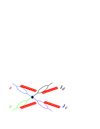
Near $z=1$, we can invoke the principles of quantum mechanical incoherence mentioned above: that the evolutions of the final state jets decouple, not only from the hard scattering, but also from each other. This allows us to “refactorize” the hard scattering function $\omega$ in Eq. (8) into convolutions of functions involving the initial, and also the final state jets, as well as soft radiation between the jets. As announced above, such a refactorization leads to new equations for evolution, and to resummation, in this case of the singular terms in $1-z$ of Eq. (9). The result is most easily exhibited for Mellin moments of $\omega$, which exponentiate, in terms of an anomalous dimension $A(\alpha_{s})$:

$${\ln}\left\{\int_{0}^{1}dzz^{N-1}\omega_{a\bar{a}\to F}(z,\mu)\right\}$$ (10)

$$=-2\int_{0}^{1}dz{z^{N-1}-1\over 1-z}\int_{(1-z)^{2}Q^{2}}^{\mu^{2}}{dm^{2}\over m^{2}}A_{a}(\alpha_{s}(m))$$

$$\sim 2\int_{Q^{2}/N^{2}}^{\mu^{2}}{dm^{2}\over m^{2}}A_{a}(\alpha_{s}(m))\,\ln\left({Nm\over Q}\right)\,.$$

This turns out to produce an enhancement in the cross section, which can be large in certain circumstances, but which is often quite modest. It shows how, even in the presence of singular corrections such as (9), next-to-leading order calculations in factorized cross sections can still give reliable answers. Another use of threshold resummation is that it automatically organizes, and hence reduces, factorization scale dependence from higher orders. We can see how this comes about by recalling that, as in Eq. (4) above, evolution results from the complementary variations of the hard and soft functions in a factorized cross section. Taking the derivative of the resummed hard function in Eq. (10), we find

$${d\ln\omega_{a\bar{a}}(z)\over d\ln\mu^{2}} \sim {2A_{a}(\alpha_{s})}\ln N$$ (11)

$$\sim -{d\ln[\tilde{f}_{a/A}\tilde{f}_{\bar{a}/B}]\over d\ln\mu^{2}}\,,$$

in terms of moments of the PDFs, $\tilde{f}$. By consistency with Eq. (4), the function $A$ that appears in the resummation formula must be the same function that appears in the $1/[1-z]_{+}$ term in the splitting functions. At NLO, the left-hand relation in Eq. (11) holds only to order $\alpha_{s}$, the first term in the expansion of $\ln\omega$, while for the resummed cross section it holds to all orders. This leads to an important reduction in factorization scale dependence compared to NLO [12, 13, 14].

4.2 Color Mixing

The result (10) shows only the leading logarithms organized by threshold resummation. Beyond leading log, threshold resummation also sheds an interesting light on the evolution of color from short to long distances. The evolution equations that lead to the resummation involve a “refactorization scale”, $\mu^{\prime}$, that separates the final state jets from the hard scattering. Like the standard factorization scale, $\mu^{\prime}$ can vary, in this case between the jet masses, $m[J_{i}]$ and the hard scale, $Q$, as illustrated in Fig. 5.

         

Figure 5: The refactorization scale.

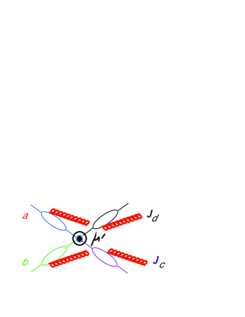
As $\mu^{\prime}$ varies, virtual gluons near scale $\mu^{\prime}$ pass between the hard scattering, and the radiation from the jets. The hard scattering, however, involves color exchange in general, and as gluons move in and out of the short-distance function, the color exchange seen at long distances changes. This leads to a matrix evolution equation beyond leading logarithm, which governs how color is radiated from short to long distances [15]. From the effective theory point of view, the hard scattering is an elementary vertex that requires renormalization, and the matrix in the evolution equation is the anomalous dimension matrix of that vertex.

As an example, we may consider quark pair annihilation into gluons, a reaction of importance for high-$p_{T}$ jets at the Tevatron. Here a color basis for the reaction consists of $s$-channel singlet, and two $s$-channel octets, of the forms $d^{ijk}T_{k}$ and $f^{ijk}T_{k}$, where $T_{k}$ is a (Gell-Mann matrix) generator of SU(3) in the fundamental (quark) representation, and where $f$ and $d$ are the antisymmetric and symmetric matrices of the SU(3) algebra, respectively. The $T$’s couple the color indices of the incoming quark pair, and $d$ or $f$ those of the outgoing gluons. The anomalous dimension matrix for this vertex turns out to be

$$\Gamma_{S^{\prime}}=\frac{\alpha_{s}}{\pi}$$ (12)

$$\times\left(\begin{array}[]{ccc}0&0&U-T\vspace{2mm}\\ 0&{C_{A}\over 2}(U+T)&{C_{A}\over 2}(U-T)\vspace{2mm}\\ 2(U-T)&{N^{2}-4\over 2N}(U-T)&{C_{A}\over 2}(U+T)\vspace{2mm}\end{array}\right)\,,$$ (16)

with $T$ and $U$ defined in terms of the scattering angle $\theta$, by $T,U\sim\ln(1\mp\cos\theta)$. The resummation of next-to-leading logarithms is best carried out by going to a diagonal basis for this matrix, with a result of the form

$$\exp\left\{-\int_{Q/N}^{Q}{dm\over m}\;\left[\lambda_{j}(\alpha_{s}(m))\right]\right\}\,,$$ (17)

where $j$ labels an eigenvector of the color exchange matrix, $\Gamma_{S}$, and where the $\lambda$’s are the corresponding eigenvalues. The same analysis may be carried out for any partonic reaction, in particular, for $g+g\rightarrow g+g$, where the coupling of the octet gluons leads to a 9$\times$9 matrix (which can be reduced to $8\times$8 [15]). Precisely the same matrix of anomalous dimensions appears in the calculation of the two loop gluon scattering amplitude [5] mentioned above, where it controls poles in dimensional regularization of the $gg\rightarrow gg$ scattering amplitude, through the function [16]

$$I^{(1)}(\epsilon)(s=\mu^{2}_{R}) \sim \left({1\over\epsilon^{2}}+{\beta_{0}\over N_{c}\epsilon}\right)\,\Gamma_{S}\,.$$ (18)

This connection strongly suggests that a combination of resummation analysis with explicit calculations can lead to further insights.

5 POWER CORRECTIONS:
UNIVERSALITY AND BEYOND

One feature of threshold resummation that we haven’t yet emphasized is that, for $z$ close enough to one, the $m^{2}$ integral on the right-hand side of Eq. (10) goes through $\Lambda_{\rm QCD}$, where the perturbative running coupling that appears in function $A$ become undefined. At $m=\Lambda_{\rm QCD}$, the perturbative expression $\alpha_{s}(m)\sim 2\pi/b_{0}\ln(m/\Lambda_{\rm QCD})$ actually has a pole, commonly referred to as its “Landau pole”, by analogy to the corresponding pole in the QED running coupling at very large momentum. At this scale, perturbation theory is not self-consistent, but can be used to identify nonperturbative corrections that restore self-consistency. In this talk, of course, I cannot do justice to the various approaches to the subject, but I’ll try to give something of the spirit.

5.1 Resummed Thrust

The approach I’ll take starts with a resummed cross section for $\rm e^{+}e^{-}\rightarrow Z^{*}(Q)\rightarrow F$. In the “elastic” limit for $F$, with two jets of invariant masses $m_{i}\ll Q$, we have

$$1-T\sim(m_{1}^{2}+m_{2}^{2})/Q^{2}\rightarrow 0\,,$$ (19)

where $T$ is the thrust. The configuration is illustrated in Fig. 6.

             

Figure 6: Z decay into two jets.

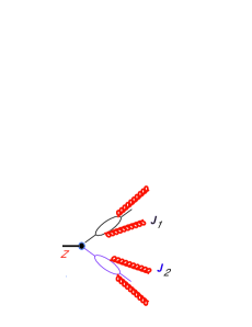
As in our discussion of threshold resummation, light-like relative velocities between the jets imply factorization. This leads to evolution and thus to a cross section resummed in logarithms of $t\equiv 1-T$,

$${1\over\sigma_{\rm tot}}\,{d\sigma_{\rm PT}(1-T)\over dT} \sim$$

$${d\over dT}\;\exp\;\left[-\int_{t}^{1}{dy\over y}\int_{y^{2}Q^{2}}^{yQ^{2}}{dm^{2}\over m^{2}}\;A(\alpha_{s}(m))\right]\,,$$

where $A(\alpha_{s})$ is the same function as in threshold resummation.

5.2 From the Resummed Cross Section
to Power Corrections

In the resummed cross section of (5.1), the Landau pole appears in the limit $y\rightarrow 0$. The following form generalizes the leading logarithm result:

$$\int_{0}^{1}dy{{\rm e}^{y/t}-1\over y}\int_{y^{2}Q^{2}}^{yQ^{2}}{dm^{2}\over m^{2}}\;A_{q}(\alpha_{s}(m))$$

$$\sim{{2\over tQ}\int_{0}^{Q^{2}}dm\;A_{q}(\alpha_{s}(m))}$$

$$+{\sum_{n=2}^{\infty}{1\over nn!}\int_{0}^{Q^{2}}{dm^{2}\over m^{2}}\left({m\over tQ}\right)^{n}\;A_{q}(\alpha_{s}(m))}$$

$$-{\sum_{n=2}^{\infty}{1\over nn!}\int_{0}^{Q^{2}}{dm^{2}\over m^{2}}\left({m^{2}\over tQ^{2}}\right)^{n}\;A_{q}(\alpha_{s}(m))}\,.$$

In this expanded form, the range of integration, $m\sim\Lambda_{\rm QCD}$, of each term is explicitly suppressed by a power of $Q$. The first term in the expansion is the only one that has the power $Q^{-1}$. From this point of view, it is natural to think of the $1/Q$ term as not only dominant, but also as reflecting universal properties of the strong coupling. Similar resummations can be carried out for a fairly large class of event shapes $e=1-T,B_{T},C\dots$, all constructed to vanish in the limit of narrow jets.

As a minimal approach, we consider only the first term in the expansion (5.2), noting that the coefficients of the integral over the running coupling may be different in other event shapes. Taking this into account, we define [17],

$$\lambda_{e}\sim C^{(e)}_{\rm PT}{\cal M}_{e}\int_{0}^{\mu_{0}}dk\,\alpha_{s}(k)\,,$$ (22)

where we replace the function $A(\alpha_{s})$ by the combination ${\cal M}_{e}\alpha_{s}$. The constant ${\cal M}_{e}$ incorporates certain higher-order effects that depend on the choice of $e$. The integral in (22) may be considered as a “universal” nonperturbative parameter. Its actual value, of course, depends on the upper limit, which serves as a factorization scale between perturbation theory and long distance physics.

This approach predicts a simple shift of the cross section [18],

$${d\sigma(e)\over de}={d\sigma_{\rm PT}(e-\lambda_{e}/Q)\over de}+{\cal O}\left({1\over e^{2}Q^{2}}\right)\,.$$ (23)

An interesting consequence is that the true $n$th moments of event shape $e$ are related to the perturbative predictions for the $n$th and $n-1$st moments by

$$\langle e^{n}\rangle=\langle e^{n}\rangle_{\rm PT}+n{\lambda_{e}\over Q}\;\langle e^{n-1}\rangle_{\rm PT}\,.$$ (24)

Observations of a variety of event shapes [19] fit rather well with this picture for the first moments, as illustrated by Fig. 7. At the same time, there appear to be substantial $1/Q^{2}$ corrections in second moments, such as $\langle(1-T)^{2}(Q)\rangle$, and indeed, purely perturbative descriptions can be given for the first moments [20].

      .

Figure 7: L3 data for first moments of various event shapes. The dashed line is perturbation theory, the solid line a fit based on Eq. (22)

5.3 Shape Functions

A natural generalization of (23), sensitive to corrections beyond the first term of (5.2) is a convolution [21],

$${d\sigma\over de} = \int_{0}^{eQ}d\epsilon\;f_{e}(\epsilon)\;{d\sigma_{\rm PT}(e-\epsilon/Q)\over de}$$ (25)

$$\hskip 14.22636pt+{\cal O}\left({1\over eQ^{2}}\right)\,,$$

where the nonperturbative “shape function” $f_{e}$ is independent of $Q$. It is therefore sufficient to fit $f$ at $Q=m_{Z}$ to derive predictions for all $Q$. Eq. (25) can incorporate all corrections like $1/(tQ)^{n}$ in Eq. (5.2).

The convolution in (25) may be based on effective theory for soft gluon radiation by $3\otimes 3^{*}$ sources, representing a quark pair. In this theory, radiation emerges from a product of ordered exponentials in the directions of the jets’ momenta,

$$W(0) = P\;{\rm e}^{ig\int_{0}^{\infty}d\lambda\beta_{1}\cdot A(\lambda\beta_{1})}\$$ (26)

$$\times\left[\,P{\rm e}^{ig\int_{0}^{\infty}d\lambda\beta_{2}\cdot A(\lambda\beta_{2})}\,\right]^{\dagger}\,,$$

as shown in Fig. 8.

         

Figure 8: Effective theory for soft radiation in the elastic limit. The double line represents the sources of Eq. (26).

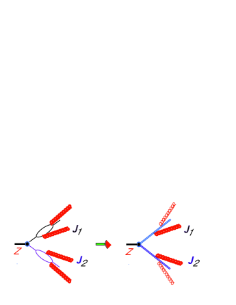
In the effective theory, true universality is at the level of correlations of energy flows, given by the matrix elements

$${\cal G}(\vec{n}_{1}\dots\vec{n}_{N}) = \langle 0|W^{\dagger}(0){\cal E}(\vec{n}_{1})\times$$ (27)

$$\times\dots\dots{\cal E}(\vec{n}_{N})W(0)|0\rangle\,,$$

where the operators ${\cal E}$ are defined to act on states by:

$${\cal E}(\vec{n})|N\rangle=\sum_{i=1}^{N}\delta^{2}(\vec{n}-\vec{n}_{i})\;E_{i}|N\rangle\,.$$ (28)

Note the close relationship of these operators to the jet energy flow operators introduced above.

For event shapes like thrust, which are related to jet masses, we need correlations of energy flow into opposite hemispheres, measured by a shape function of two variables,

$$f(\varepsilon_{L},\varepsilon_{R}) =$$

$$\langle 0|W^{\dagger}\delta(\varepsilon_{L}-{\cal E}_{L})\,\delta(\varepsilon_{R}-{\cal E}_{R})W|0\rangle\,,$$

where we define

$${\cal E}_{L,R} = \int d^{2}\vec{n}\theta(\pm\cos\theta_{n})\,(1-|\cos\theta_{n}|)\,{\cal E}(\vec{n})\,.$$

In this notation, the squared mass of a jet moving into the right (left) hemisphere is proportional to $Q\varepsilon_{R}$ ($Q\varepsilon_{L}$). The thrust event shape function is then given by

$$f_{T}(\varepsilon) = \int d\varepsilon_{R}d\varepsilon_{L}\,\delta(\varepsilon-\varepsilon_{L}-\varepsilon_{R})$$ (31)

$$\hskip 28.45274pt\times f(\varepsilon_{L},\varepsilon_{R})\,.$$

A “mean field” reduction :

$${\cal G}(\vec{n}_{1}\dots\vec{n}_{N})\to\prod_{i}\langle 0|W^{\dagger}(0){\cal E}(\vec{n}_{i})W(0)|0\rangle$$ (32)

reproduces the shift of Eq. (23), because all the shape functions reduce to the form,

$$f_{e}(\epsilon)\to\delta(\epsilon-\lambda_{e})\,.$$ (33)

In this limit, we recover the universality of Eq. (22).

The phenomenology of shape functions has been discussed in [22] and in [23], while in [24], it was shown that the double distribution determined phenomenologically in [23],

$$f(\varepsilon_{L},\varepsilon_{R}) = {\rm const}\,(\varepsilon_{L}\varepsilon_{R})^{a-1}$$ (34)

$$\times\exp\left(-{\varepsilon_{L}^{2}+\varepsilon_{R}^{2}+2b\varepsilon_{L}\varepsilon_{R}\over\Lambda^{2}}\right)\,,$$

follows from rather general considerations. In particular, it was found that the parameters in this expression have the interpretations: for $a$, the number of particles radiated per unity rapidity, and for $b$, the correlation due to a “spill-over” of radiation at the boundary of the two hemispheres from hadronization.

6 CONCLUSION

The finiteness of time limited the interesting topics that I was able to cover at Trento, and made it necessary to pass over developments in factorization for exclusive B decay amplitudes [25], in high parton density [26], in hadronic spin structure, and in uncertainties in parton distribution functions [27]. Many topics have gone unmentioned, but I hope that I have communicated part of the reason why many of us find perturbative QCD and its extensions of enduring interest.

It seems clear to me that there is much still to be learned by studying nonperturbative corrections for observables like those discussed in this talk. In some ways, event shapes related to jets are the ideal testing ground for the perturbative-nonperturbative interface. Perturbation theory is the dominant contribution, but nonperturbative effects are substantial and, more importantly, by varying the energy, and studying moments of distributions, and correlations of the kind discussed above, we should be able to “dial” the nonperturbative component. In this fashion, we may probe the evolution of this most demanding of field theories in new ways, providing insight not only into QCD, but into the enterprise of quantum field theory itself.

Acknowledgements

My thanks go to the organizers of Light Cone Physics: Particles and Strings, for their invitation, and to the European Centre for Theoretical Studies in Nuclear Physics and Related Areas for its hospitality. I would especially like to thank Antonio Bassetto, Ines Campo, Renzo Leonardi and Federica Vian, for their generous help. This work was supported in part by the National Science Foundation, grants PHY9722101 and PHY0098527.

References

- [1] S.A. Larin, P. Nogueira, T. van Ritbergen, J.A.M. Vermaseren, Nucl. Phys. B492 (1997) 338, hep-ph/9605317.
- [2] S. Moch, J.A.M. Vermaseren, M. Zhou, hep-ph/0108033.
- [3] A.L. Kataev, G. Parente, A.V. Sidorov, Nucl. Phys. B573 (2000) 405, hep-ph/9905310; W.L. van Neerven, A. Vogt, Nucl. Phys. B603 (2001) 42, hep-ph/0103123; A.D. Martin, R.G. Roberts, W.J. Stirling, R.S. Thorne, hep-ph/0201127.
- [4] Z. Bern, L.J. Dixon, D.A. Kosower, JHEP 0001 (2000) 027, hep-ph/0001001.
- [5] E.W.N. Glover, C. Oleari, M.E. Tejeda-Yeomans, Nucl. Phys. B605 (2001) 467, hep-ph/0102201.
- [6] L.W. Garland et al., hep-ph/0112081.
- [7] S. Ellis, J. Huston, M. Tonnesmann, contribution to APS / DPF/DPB Summer Study on the Future of Particle Physics (Snowmass 2001), hep-ph/0111434.
- [8] F.V. Tkachov, Phys. Rev. Lett. 73 (1994) 2405, hep-ph/9901332; Int. J. Mod. Phys. A12 (1997) 5411, hep-ph/9601308.
- [9] W.T. Giele, E.W.N. Glover, hep-ph/9712355.
- [10] C.L. Basham, L.S. Brown, S.D. Ellis, S.T. Love, Phys. Rev. Lett. 41 (1978) 1585; Phys. Rev. D17 (1978) 2298; D19 (1979) 2018; G. Sterman, Phys. Rev. D19 (1979) 3135.
- [11] N. Kidonakis, Int. J. Mod. Phys. A15 (2000) 1245, hep-ph/9902484.
- [12] E.L. Berger, H. Contopanagos, Phys. Rev. D57 (1998) 253, hep-ph/9706206.
- [13] N. Kidonakis, R. Vogt Phys. Rev. D59 (1999) 074014, hep-ph/9806526; N. Kidonakis, J.F Owens, Phys. Rev. D61 (2000) 094004, hep-ph/9912388.
- [14] S. Catani et al. JHEP 9903 (1999) 025, hep-ph/9903436.
- [15] N. Kidonakis, G. Oderda, G. Sterman, Nucl. Phys. B531 (1998) 365, hep-ph/9803241.
- [16] S. Catani, Phys. Lett. B427 (1998) 161, hep-ph/9802439.
- [17] Yu.L. Dokshitzer, A. Lucenti, G. Marchesini, G.P. Salam, JHEP 9805 (1998) 003, hep-ph/9802381.
- [18] G.P. Korchemsky, G. Sterman, 30th Rencontres de Moriond, hep-ph/9505391; Y.L. Doskshitzer, B.R. Webber, B404 (1997) 321, hep-ph/9704298.
- [19] L3 Collaboration (M. Acciarri et al.), Phys. Lett. B489 (2000) 65, hep-ex/0005045.
- [20] R. Reinhardt, U. Flagmeyer, K. Hamacher, O. Passon, D. Wicke (for the DELPHI Codllaboration), DELPHI 2001-062 CONF 490 (2001).
- [21] G.P. Korchemsky, G. Sterman, Nucl. Phys. B555 (1999) 335, hep-ph/9902341.
- [22] E. Gardi, J. Rathsman, Nucl. Phys. B609 (2001) 123, hep-ph/0103217, hep-ph/0201019.
- [23] G.P. Korchemsky, S. Tafat, JHEP 0010 (2000) 010, hep-ph/0007005.
- [24] A.V. Belitsky, G.P. Korchemsky, G. Sterman, Phys. Lett. B515 (2001) 297, hep-ph/0106308.
- [25] C.H. Chen, Y,Y, Keum, H.-n. Li, Phys. Rev. D64 (2001) 112002, hep-ph/0107165; M. Beneke, G. Buchalla, M. Neubert, C.T. Sachrajda, Nucl. Phys. B591 (2000) 313, hep-ph/0006124; C.W. Bauer, D. Pirjol, I.W. Stewart, Phys. Rev. Lett. 87 (2001) 201806, hep-ph/0107002
- [26] R. Venugopalan, 34th Rencontres de Moriond, hep-ph/9907209.
- [27] J. Pumplin et al., Phys. Rev. D65 (2002) 014013, hep-ph/0101032; D. Stump et al., ibid., 014012, hep-ph/0101051; W.T. Giele, S.A. Keller, D.A. Kosower, hep-ph/0104052.